Atmospheric neutrino challenges

Abstract

We briefly review the improvements in the predictions of atmospheric neutrino fluxes since the NOW2000 workshop. In spite of the great progress of the calculational technique the predictions are still not exact because of the uncertainties in the two major sets of input - cosmic ray flux and hadronic interactions on light nuclei.

1 INTRODUCTION

In 2004, after the experimental statistics on atmospheric neutrinos has become so good, one the major obstacles to the exact determination of the oscillation parameters is the uncertainty in the predictions of the atmospheric neutrino flux. The predictions are not bad, we qualitatively understand well all features of the neutrino flux, but reaching the necessary 5% or better level is still impossible.

The basic features of the atmospheric neutrinos are very well established. They follow from the neutrino production processes and the development of the hadronic cascades in the atmosphere. The production mechanism is the decay chains of mesons created in these cascades. Positively charged pions, for example, decay into $\mu^{+}$ and $\nu_{\mu}$. The muons subsequently decay into $\nu_{e},\;\bar{\nu}_{\mu}$ and $e^{+}$. Since pion decays dominate the atmospheric neutrino production in the sub-GeV energy range, one can immediately predict the flavor ratio ${{\nu_{\mu}\;+\;\bar{\nu}_{\mu}}\over{\nu_{e}\;+\;\bar{\nu}_{e}}}$ = 2.

The decay chain also determines the neutrino energy spectra. In the atmosphere mesons encounter the interaction–decay competition. Thus neutrinos from meson decay will have a spectrum one power of energy steeper than the primary cosmic ray spectrum. The muon daughter neutrinos will have a spectrum steeper by two powers of energy, because the muon spectrum itself is steeper by $1/E$. Electron neutrinos thus have approximately $E^{-4.7}$ differential spectrum. Muon neutrino spectra are flatter. At low energy, however, the spectra are significantly flatter (parallel to the primary cosmic ray spectrum) as all mesons and muons decay. At high energy the neutrino spectrum is modified by the increasing kaon contribution, which asymptotically reaches 90%. The contribution of charm and heavier flavors is still not essential.

Neutrino energy spectra are a function of the zenith angle of the atmospheric cascades. Mesons in inclined showers spend more time in tenuous atmosphere where they are more likely to decay rather than interact. For this reason the spectra of highly inclined neutrinos are flatter than those of almost vertical neutrinos.

The general expectation is for up–down symmetric neutrino fluxes. The shorter distance to the atmosphere above a detector is compensated by the smaller amount of atmosphere per unit solid angle - both follow the $R^{2}$ law. The symmetry is broken by the existence of geomagnetic field that prevents low energy cosmic rays from entering and interacting in the atmosphere in regions of low geomagnetic latitude. Such is the case in Japan where more low energy atmospheric neutrinos enter the detector from below than from above. The symmetry should be restored at neutrino energies above 10 GeV (cosmic rays above 50 GeV) which are not affected by geomagnetic effects.

There are two basic sets of inputs in a prediction of the atmospheric neutrino flux:
– Energy spectrum and composition of the cosmic ray flux. The cosmic ray composition affects the ratio of neutrinos and antineutrinos, thus the rate of neutrino events because of the different $\nu$ and $\bar{\nu}$ cross sections.
– Hadronic interactions on light nuclei (atmosphere) and particle production features in a wide energy range - from 1 to 10⁵ GeV in the Lab.

Neither of these sets of inputs has uncertainty of less than 10%. Uncertainty estimates give higher values. This is the basic reason for which the predictions of the atmospheric neutrino flux is a challenge.

2 GEOMETRY OF ATMOSPHERIC NEUTRINO PRODUCTION

Until recently, before NOW2000, all analyses of the atmospheric neutrino data were performed with the use of 1D calculations, such as Refs. [1, 2, 3]. These predictions are made with the assumption that all neutrinos follow the direction of the primary cosmic rays. Geomagnetic field was only applied to the geomagnetic modification of the cosmic ray spectra at different locations as a function of the particle zenith angle. The situation now is quite different. There are more than seven independent calculations performed by different [4, 5, 6, 7, 8, 9, 10, 11, 12, 13] groups.

Figure 1: Illustration of the 3D geometry for neutrino production angle 30^∘ and different neutrino production heights.

The geometry of the atmospheric neutrino production was first treated analytically and numerically by Lipari [14, 15], who demonstrated that it is indeed very different from the 1D approximation. In the realistic case when all secondary particles in the atmospheric cascades are produced with transverse momenta the neutrino angular distribution does not exactly follow that of the interacting cosmic rays. A vertical interacting cosmic ray generates neutrinos that are more inclined and the effect is not compensated by cosmic rays of higher inclination. The strength of the effects depends on the angle between the primary nucleon and the secondary mesons and on the height of the neutrino production layer in the atmosphere. Figure 1 illustrates the effect for different production heights. There is a peak of neutrinos around the horizon and a decrease of the neutrino flux at zenith angles less than 60^∘. The total number of low energy neutrinos is somewhat higher than in the 1D approximation.

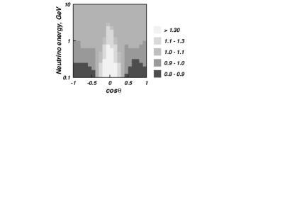
Figure 2: Importance of the 3D effects at Kamioka in the $E_{\nu}$ $\cos{\theta_{\nu}}$ plane.

It is obvious that the effect is strong at low neutrino energy - 30^∘ production angle requires $p_{\bot}/p_{\|}$ ratio of $\tan{{\rm 30^{\circ}}}$ = 0.58, i.e. relevant only for low energy interactions. At neutrino energies above 10 GeV, when neutrinos are produced under very small angle, the effect totally disappears. In practical terms the 3D effects are not important above neutrino energy of about 3 GeV. Figure 2 shows the importance of the 3D effects in the energy/angle plane of the atmospheric neutrinos. The biggest effect, an increase of the neutrino flux by more than 30% is at the horizon for $E_{\nu}$ less than about 0.5 GeV. The vertical neutrino fluxes below 0.3 GeV are decreased by up to 20%. Fluxes for zenith angles around 60^∘ are not changed by more than a couple of per cent.

At energies above 1 GeV there is only a slight (less than 10%) increase of the fluxes below 3 GeV. At higher energy the effects totally disappear.

In spite of the greater sophistication of the modern 3D calculations, most of the computer codes have to use several simplifications. These include the treatment of the atmospheric density profile, which is often treated as a single uniform profile (with exception of Ref. [7]). Another is the altitude of the Earths surface, which is of course different from sea level. The same is true for the altitude of the real detector for which the prediction is made - the SuperKamiokande detector is at about 3 km higher altitude than SNO. A higher detector is obviously exposed to a slightly smaller flux of downgoing neutrinos. The most important simplification if the size of the neutrino detector in the Monte Carlo simulation which is often bigger than 1000 km. Using very big detectors does not allow a correct account for the local geomagnetic effects. An interesting problem is the treatment of the low Monte Carlo statistics of very inclined almost horizontal neutrinos, which can bring very large uncertainty in the result.

All these (and probably other) simplifications are necessary because of the very high ratio of the area of the Earths atmosphere to the area of even a huge detector. Their effects and not very well known and need a careful exploration. They do not, however, contribute heavily to the uncertainties in the neutrino prediction. These are dominated by the uncertainties in the basic inputs.

3 PROBLEMS WITH THE BASIC INPUTS

Ten years ago the situation was worse: different measurements of the cosmic ray flux at about 10 GeV were different by about 50%. The situation has since improved, but not as much as we would like.

3.1 Cosmic Ray Spectrum

The agreement of the AMS [16] and BESS[17] data on cosmic ray protons (Hydrogen nuclei) was considered (and it is) a break through. Protons are by far the most important cosmic ray nuclei in the energy range below 1000 GeV. They contribute 78% of the all nucleon flux at 10 GeV, compared with the 15% contribution of He and the total of 8% contribution of all heavier nuclei. The better than 1% agreement between the AMS and BESS results promised a serious improvement in our knowledge of the cosmic ray flux.

The fluxes assigned to the He flux by these two experiments do not agree that well, but the agreement is still better than 10%. The problem is that there are other measurements, particularly the CAPRICE results [18] that are lower by about 20% for both protons and He fluxes. Since the statistical and systematic errors given by the experimental groups are significantly lower than these differences one can not put together and fit all experimental data. The decision has then to be made: which experiments are good and which are not. I believe that scientists outside the experimental group should not attempt to declare an experiment more or less worthy. The only thing we can do is to increase the size of the uncertainty on the cosmic ray flux.

Including the contribution of heavier nuclei and extending the cosmic ray flux models to 10⁵ GeV presents more problems of similar character. Since it looks that heavy nuclei have a flatter energy spectrum than protons it is quite possible than at energies above 10 TeV/nucleon the all nucleon spectrum could be dominated by the contribution of nuclei with $Z>1$. This will change the cosmic ray composition - the ratio of primary protons and nucleons interacting in the atmosphere. As an example we present in Fig. 3 the all nucleon spectra derived in 1996 in Ref. [3] and in 2001 in Ref. [19]. The latter derivation does not include CAPRICE data.

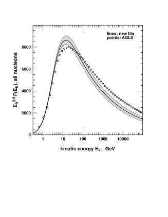
Figure 3: All nucleon spectra derived before (AGLS) and after the publication of the AMS and BESS data. The shaded area gives the derived uncertainties.

At 10 GeV the newly derived flux is higher than the older parametrization by about 15%. The two parametrizations cross over at about 50 GeV and the old parametrization is higher than the new one by more than 40% at 10⁵ GeV. There are several reasons for the steeper all nucleon spectrum in the new fit. To start with, the highest energy several points in AMS and in BESS show a steep spectrum and with their lower errors dominate any fit. Secondly, the fluxes in the new TeV measurement, RUNJOB [20], are lower than JACEE [21]. That combination of high and low obviously requires a steeper spectrum.

It is not difficult to predict qualitatively what the effect of these two parameterizations is on the predicted neutrino fluxes. The new sub-GeV neutrino fluxes will be higher by 10-20% while the high energy neutrinos, which are responsible for the upward going muon events, will be lower.

One has to be very careful and inventive and use limits from different experiments to constrain the flux models. As an example, the model of Ref. [19] generates all particle flux at 10⁵ GeV that is low compared to the estimates of the all particle flux from air shower measurements.

3.2 Particle Production

The situation with the hadronic interaction models is not any better. There are a few measurements of the particle production on light nuclei, most of them on Be. Measurements were done when new neutrino beams were designed at accelerators. Most available data sets are from the 60’s and the early 70’s when the measurements were performed with single arm spectrometers, and correspondingly cover only a part of the phase space. In the absence of applicable theory low energy hadronic interaction models are compiled to fit one or the other set of experimental data. Figure 4, compiled from Fig. 15 of Ref. [24], gives an idea how different these models can be.

Figure 4: Predictions of four interaction models are compared to 24 GeV p-Be$\rightarrow$p data of Refs. [22, 23]. See Ref. [24] for all references.

DPMjet and FLUKA are qualitatively consistent (since FLUKA started as an extension of earlier DPMjet version). The homegrown model of the Bartol group, Target 2.1, is not very different from Fritiof 1.6, which is just an attempt to fit the data points shown in Fig. 4.

Fig. 5 plots the $\pi^{-}$ production spectra in 24 GeV p-Be interactions predicted by Target 2.1 and FLUKA in comparison with experimental data.

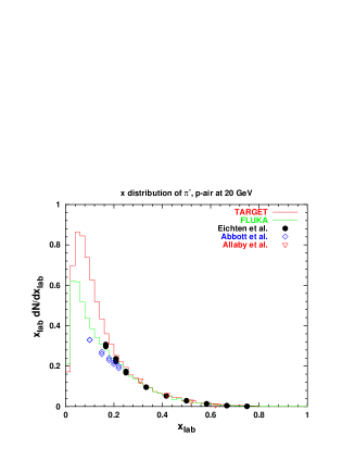
Figure 5: Predictions of two interaction models are compared to 24 GeV p-Be$\rightarrow\;\pi$ data of Refs. [22, 23, 25].

The differences between the two interaction models are significant. Visual inspection seems to show that Target 2.1 is a good description at high momenta, but may overestimate the pion production at low $x$ values. E-802 data favor the lower pion production model.

At energies above 100 GeV the problems are different and the main problem is the K/$\pi$ ratio as a function of energy. A large part of the problem is the associated $\Lambda K$ production that generates hard positive kaons. The production cross section is measured directly as well as by the $K^{+}/K^{-}$ ratio. Models with large $\Lambda K$ production cross section predict high neutrino fluxes above about 100 GeV, where the kaon contribution is already high [24].

4 UNCERTAINTIES

A recent study of the uncertainties in the prediction of the atmospheric neutrino fluxes from different hadronic interaction models was performed by Giles Barr (private communication). The conclusions are that not all important atmospheric neutrino features are strongly affected by the model uncertainty. Flavor ratios ($\nu_{e}/\bar{\nu}_{e},\;\nu_{\mu}/\bar{\nu}_{\mu},\;(\nu_{\mu}+\bar{\nu}_{\mu})/(\nu_{e}/\bar{\nu}_{e})$) are stable to better than 1% at $E_{\nu}$ less than 30 GeV. At higher energies the uncertainties may reach 10%. The up/down symmetry has a different behavior. Its uncertainty below 1 GeV if order 5%, decreases to 1% or less between 1 and 10 GeV and then grows again to about 5% at higher energy.

The absolute normalization is a different story that depends on the cosmic ray flux as well as on the interaction model. It is illustrated in Fig. 6 which compares the calculations of Refs. [9, 13, 12] with the use of the same cosmic ray spectrum.

Figure 6: Ratio of muon neutrino fluxes calculated by Refs. [13] (solid) and [9] to the fluxes of Ref. [12].

It is obvious that the Bartol calculation gives the highest high energy neutrino flux. Up to energy of 10 GeV the Honda et al. calculation [13] is on the 95% level and declines further at higher energy. The FLUKA calculation is lower than Bartol’s already below 1 GeV and the difference increases to more than 20% when approaching energy of 1000 GeV.

Such differences affect mostly the analysis of the upward going neutrino induced muon data, which depend on the neutrino flux of energy up to 10 TeV, where the differences could even be bigger. Figure 7 shows the angular distribution of upward going neutrino induced muons calculated with the fluxes of FLUKA [9] and Agrawal et al. [3]. The new Bartol fluxes are not used because currently they do not extend above 1000 GeV.

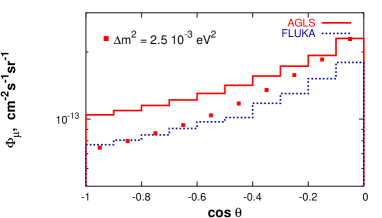
Figure 7: Angular distribution of upward going neutrino induced muons at Kamiokande without oscillations - histograms. Points show Bartol’s flux with oscillations ($\Delta m^{2}$ = 0.0025 eV²).

The situation can be really confusing when the data (assuming it has the same shape as in our calculation) agrees with Bartol flux in horizontal direction and with FLUKA for vertical events without an account for oscillations. Although the Agrawal et al. [3] flux, that was obtained with the old flux model in Fig. 3, is higher than any other calculation the MACRO collaboration (see G. Giacomelly in these Proceedings) concludes that the new 3D calculations [9, 13] differ [26] from the global fit of their neutrino data.

5 SUMMARY

The current situation with the predictions of the atmospheric neutrino fluxes is not ideal - the progress in theory seems to be behind that of experiments. On the other hand, there is a big improvement in the calculational technique, which will eventually lead to significantly better results.

To achieve significantly better predictions we need much better input data on both the cosmic ray flux and on the hadronic interactions on light nuclei.

The current program on studies of cosmic ray flux with balloon instruments is strong, and we hope that these regular flights will continue during the next several years. We also expect the satellite flights of the PAMELA and AMS experiments, that should be able to measure the cosmic ray flux even better. The keys are the achievement of understanding about the absolute normalization of different experiments and the extension of direct measurements with the same instruments to energies above several TeV/nucleon.

The hope for improvement of the hadronic interaction models is once again linked to the new neutrino beams that are prepared in both CERN and Fermilab. Parts of that preparation are the experiments HARP and P322 (using the NA49 detector) at CERN and MIPP (E907) at Fermilab. HARP is in the process of data analysis, and P322 has had two runs at 100 and 160 GeV. It would be a significant improvement over the past if the results of these experiments agree with each other.

The future is not bleak, but we do have a lot of work to do.

Acknowledgment This talk was based on work performed with G.D. Barr, R. Engel, T.K. Gaisser, P. Lipari and others.

References

- [1] M. Honda et al., Phys. Rev. D52, 4985 (1995)
- [2] G. Barr, T.K. Gaisser & T. Stanev, Phys. Rev., D39, 3532 (1989)
- [3] V. Agrawal et all., Phys. Rev. D53, 1314 (1996)
- [4] G. Battistoni, et al., Astropart. Phys., 12, 315, (2000)
- [5] M. Honda et al., Phys. Rev. D64:053011 (2001)
- [6] Y. Tserkovnyak et al., Astropart. Phys., 18, 449 (2003)
- [7] J. Wentz et al., Phys. Rev. D67:073020 (2003)
- [8] V. Plyaskin, Phys. Lett. B516 (2001) 213
- [9] G. Battistoni et al., Astropart.Phys.19, 269 (2003); Erratum-ibid.19, 291 (2003)
- [10] J. Favier, R. Kossakowski and J.P. Vialle, Phys. Rev. D68:093006 (2003)
- [11] Y. Liu, L. Derome and M. Bu’enerd Phys. Rev. D67:073022 (2003)
- [12] G.D. Barr et al., Phys. Rev., D70:023006 (2004)
- [13] M. Honda et al., Phys. Rev. D70:043008 (2004)
- [14] P. Lipari, Astropart. Phys. 14 (2000) 153
- [15] P. Lipari, Astropart. Phys. 14 (2000) 171
- [16] J. Alkaraz et al., Phys. Lett., B490, 27 (2000)
- [17] J.Z. Wang et al., Ap. J., 564, 244 (2002)
- [18] M. Boezio et al., Astropart. Phys. 19, 583 (2003)
- [19] T,K, Gaisser et al., Proc. 27th ICRC (Hamburg), 5, 1643 (2001)
- [20] A.V. Apanasenko et al., Astropart. Phys., 16, 13 (2001)
- [21] K. Asakimori et al., Ap. J., 502, 278 (1998)
- [22] T. Eichten et al., Nucl. Phys. B44, 333 (1972).
- [23] J.V. Allaby et al. CERN Yellow Report 70–12.
- [24] T.K. Gaisser & M. Honda, Ann. Rev. Nucl. Part. Sci., 52, 153 (2002)
- [25] T. Abbott et al., Phys.Rev. D45, 3906 (1992)
- [26] M. Ambrosio et al., Eur. Phys. J., C36, 323 (2004)