The problem of small and large scale fields in the solar dynamo

Abstract

Three closely related stumbling blocks of solar mean field dynamo theory are discussed: how dominant are the small scale fields, how is the alpha effect quenched, and whether magnetic and current helicity fluxes alleviate the quenching? It is shown that even at the largest currently available resolution there is no clear evidence of power law scaling of the magnetic and kinetic energy spectra in turbulence. However, using subgrid scale modeling, some indications of asymptotic equipartition can be found. The frequently used first order smoothing approach to calculate the alpha effect and other transport coefficients is contrasted with the superior minimal tau approximation. The possibility of catastrophic alpha quenching is discussed as a result of magnetic helicity conservation. Magnetic and current helicity fluxes are shown to alleviate catastrophic quenching in the presence of shear. Evidence for strong large scale dynamo action, even in the absence of helicity in the forcing, is presented.

brandenb@nordita.dk

1 Introduction

Over the past 30 years, the standard approach to understanding the origin of the solar cycle has been mean field dynamo theory. This approach can be justified simply by the fact that the sun does have a finite azimuthally averaged mean field, $\overline{\vec{B}}(r,\theta,t)$, where $r$ and $\theta$ are radius and colatitude. Observationally, we really only know with some certainty its radial component at the surface, $\overline{B}_{r}(R,\theta,t)$, where $R$ is the radius of the sun. There is also some indirect evidence for the toroidal field, $\overline{B}_{\phi}(r_{\rm spot},\theta,t)$, where $r_{\rm spot}$ is the not well known radius where sunspots are anchored. Both components give a very clear indication of the spatio-temporal coherence of the mean field, with a 22 year cycle and latitudinal migration.

Mean field theory has certainly been successful in showing that a solar-like mean field can be produced if there is an $\alpha$ effect, i.e. if the mean electromotive force has a component along the mean field (Weiss 2005). A number of complications have arisen in the mean time.

• The standard theory for calculating the value of $\alpha$ and other relevant transport coefficients (such as turbulent magnetic diffusivity) relies on the first order smoothing (FOSA) or second order correlation approximation (SOCA). This approach is valid if either the magnetic Reynolds number is small (poor microscopic conductivity of the gas) or if the so-called Strouhal number (Käpylä et al. 2005) is small compared to unity. The latter means that the correlation time is supposed to be much less than the turnover time of the turbulence, which is not usually the case. The former assumption is equally inappropriate.

• Shortly after mean field theory became popular there have been recurrent concerns about its applicability when the field strength is comparable to the equipartition value of the turbulence, i.e. if the magnetic energy is comparable to the kinetic energy of the turbulence. Such concerns where first addressed by Piddington (1970, 1972), but more recently by Vainshtein & Cattaneo (1992) and Kulsrud & Anderson (1993).

• In more recent years the problem of the resistively slow evolution of magnetic helicity has been discussed in connection with a correspondingly slow saturation if the dynamo (Brandenburg 2001, Mininni et al. 2003). This resistively slow time scale in the problem can also affect the cycle period in an $\alpha\Omega$ dynamo (Brandenburg et al. 2001, 2002). The presence of boundaries may help (Blackman & Field 2000a,b, Kleeorin et al. 2000, 2002, 2003), but it may also make matters worse (Brandenburg & Dobler 2001). The question is therefore whether suitably arranged shear is needed to transport magnetic helicity out of the domain (Vishniac & Cho 2001, Subramanian & Brandenburg 2004). The indications are that with shear and open boundary conditions the otherwise catastrophic $\alpha$ quenching can be alleviated (Brandenburg & Sandin 2004).

In the following we discuss the current status on all three issues. Indeed, there has been a lot of progress, and from an optimistic viewpoint one might almost think that these issues have now been solved. But, of course, as always in science, new problems and unexpected issues emerge all the time. Also, having proposed one solution to a problem does not exclude alternative solutions, and so only with time will we be able to look back and say how it really was.

2 Problem I: dominance of small scale fields?

The first issue of the relative importance of small scale versus large scale fields can be discussed in terms of the magnetic energy spectrum. We begin with a historical perspective.

2.1 Turbulent diffusion and turbulent cascade

Turbulent diffusion relies on the ability of the turbulence to transport energy from large scales to small scales. This is an important consideration that was discussed by Stix (1974) in the context of early criticism raised against dynamo theory. The situation is illustrated in Fig. 1.

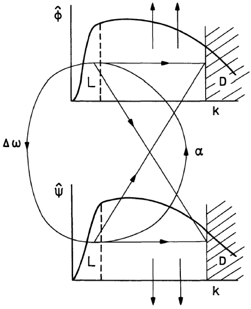
Figure 1: A sketch from the original review by Stix (1974) where he illustrates the role of a turbulent cascade in converting large scale poloidal and toroidal flux into small scale fields where it can be converted into heat by microscopic resistivity.

The assumption of a magnetic energy spectrum being parallel or even coincident with that of kinetic energy, and this being equivalent to the cascade in ordinary (nonmagnetic) turbulence is natural, but not trivial and not fully confirmed by simulations, as will be discussed in the next section.

2.2 Numerical indications for a magnetic cascade

Over the past decades some steady progress has been brought about; see Fig. 2, where we show kinetic and magnetic energy spectra from Meneguzzi et al. (1981), Kida et al. (1991), Maron & Cowley (2001), representing the improvement of the state of the art simulations over the past three decades. The spectra from all three papers show that at large scales the spectral magnetic energy is below the spectral kinetic energy. In the spectra of Meneguzzi et al. (1981) and Maron & Cowley (2001) the spectral magnetic energy peaks at about $k\approx 5$. However, there has not really been any evidence for power law behavior. One exception is the spectrum obtained by Kida et al. (1991) who find a $k^{0}$ spectrum, but this has not been found in subsequent simulations by Maron & Cowley (2001) or Maron et al. (2004), for example. The numerical resolution used in the three cases is $64^{3}$, $128^{3}$, and $256^{3}$ meshpoints, respectively. Obviously, much higher resolution is needed to begin to address the possibility of powerlaw behavior. This was the main reason for Haugen et al. (2003) to push the resolution to $1024^{3}$ meshpoints; see Fig. 3. Based on these results, one can begin to see the development of what looks like an inertial range with a tentative $k^{-3/2}$ scaling. If this is confirmed, it would rule out earlier claims that the magnetic energy spectrum peaks at the resistive scale (Maron & Blackman 2002, Schekochihin et al. 2002). However, the results by Haugen et al. (2003) are still open to alternative interpretations. Schekochihin et al. (2004a) have argued that the magnetic spectrum is still curved, and that there is therefore actually no evidence for powerlaw behavior. So, the asymptotic spectral behavior of hydromagnetic turbulence is still very much an open question.

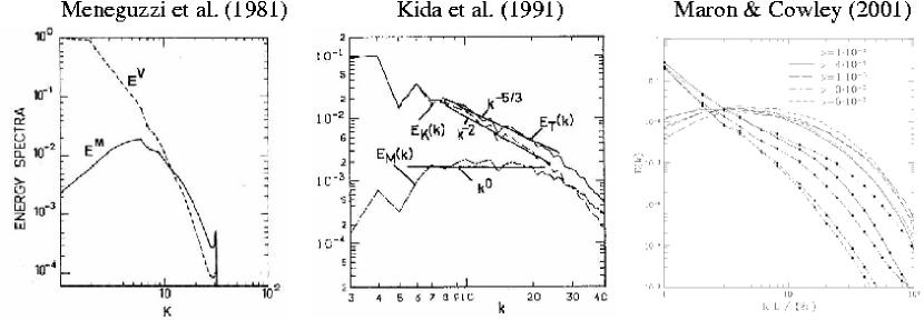
Figure 2: Steady progress in solving the small scale dynamo problem. Kinetic and magnetic energy spectra from the papers by Meneguzzi et al. (1981), Kida et al. (1991), and Maron & Cowley (2001). The numerical resolution used in the three cases is $64^{3}$, $128^{3}$, and $256^{3}$ meshpoints, respectively. All spectra agree in that at large scales (small wavenumbers $k$) the spectral magnetic energy is below the spectral kinetic energy. In the spectra of Meneguzzi et al. (1981) and Maron & Cowley (2001) the spectral magnetic energy peaks at about $k=5$.

A puzzling aspect of all the magnetic energy spectra is the excess of spectral magnetic energy over spectral kinetic energy. In order to get some insight into the possible asymptotic behavior, Haugen & Brandenburg (2004) have recently considered simulations with subgrid scale modeling using either hyperviscosity or Smagorinsky viscosity together with magnetic hyper-resistivity.

Consider for comparison first the purely hydrodynamic case (Fig. 4), where we can use the high resolution simulations of Kaneda et al. (2003) on the Earth Simulator as benchmark. This simulation corresponds to a resolution of $4096$ collocation points. Note that there is not even a clear confirmation of the famous Kolmogorov $k^{-5/3}$ spectrum, but there is a $k^{-0.1}$ correction in what looks like the inertial range. However, simulations with both hyperviscosity (Haugen & Brandenburg 2004) and Smagorinsky subgrid scale modeling (Haugen & Brandenburg, in preparation) confirm this correction to the inertial range; see Fig. 4.

Figure 3: Magnetic, kinetic and total energy spectra. $1024^{3}$ meshpoints. The Reynolds number is $u_{\rm rms}/(\nu k_{\rm f})\approx 960$. [Adapted from Haugen et al. (2003).]

Figure 4: Comparison of energy spectra of the $4096^{3}$ mesh points run of Kaneda et al. (solid line) and $512^{3}$ mesh points runs with hyperviscosity (dash-dotted line) and Smagorinsky viscosity (dashed line).

The uprise in the compensated power spectra just before the dissipative subrange is due to the bottleneck effect in turbulence (Falkovich 1994). This effect is much weaker in wind tunnel turbulence (She & Jackson 1993), but this is because these are one-dimensional spectra, $E_{\rm 1D}(k)$, which are related to the fully three-dimensional spectra via a simple integral transformation

$$E_{\rm 1D}(k)=\int_{k}^{\infty}{E_{\rm 3D}(k^{\prime})\over k^{\prime}}\,{\rm d}{}k^{\prime}.$$ (1)

Of course, for perfect power law spectra the two are the same, but they can be quite different when there are departures from power law behavior, such as due to the bottleneck effect itself and due to the dissipative subrange (Dobler et al. 2003).

In Fig. 5 we show the results for the hydromagnetic case where we have used hyperresistivity and either hyperviscosity or Smagorinsky subgrid scale modeling for the velocity field. There are two important things to notice. First, the compensated magnetic spectrum seems flat, but the kinetic energy spectrum seems to rise, possibly approaching the magnetic energy spectrum. A sketch of what we believe the asymptotic magnetic and kinetic energy spectra could look like is shown in Fig. 6.

Figure 5: Magnetic and kinetic energy spectra for runs with $512^{3}$ mesh points and hyperviscosity and hyper-resistivity (solid line) and Smagorinsky viscosity and hyper-resistivity (dashed line). Note the mutual approach of kinetic and magnetic energy spectra before entering the dissipative subrange.

Figure 6: Sketch of the anticipated kinetic and magnetic energy spectra in the large Reynolds number limit for $\mbox{\rm Pr}_{M}=1$. Note the slight super-equipartition just to the right of the peak of $E_{\rm M}(k)$ and the asymptotic equipartition for large wavenumbers.

In summary, there seems now some evidence suggesting that there is indeed a magnetic energy cascade. We should emphasize, however, that most of the simulations to date have either unit magnetic Prandtl number, or at least magnetic Prandtl numbers that are not very different from unity.

Figure 7: Dependence of the critical magnetic Reynolds numbers as a function of the magnetic Prandtl number using for the direct simulations (Haugen et al. 2004), indicated by diamonds, compared with results using hyperviscosity (asterisks) or Smagorinsky viscosity (triangles).

The question of the magnetic Prandtl number dependence is potentially quite important for stars where this number is very small (magnetic diffusivity much larger than the kinematic viscosity). Using a modified Kazantsev model, Rogachevskii & Kleeorin (1997) pointed out that when the velocity field displays Kolmogorov scaling near the resistive cutoff wave number, the dynamo becomes much harder to excite than for a velocity field that shows significant power only at large scales. They found that the critical magnetic Reynolds number for dynamo action can exceed a value of 400, which is about 10 times larger than the critical value of 35 for unit magnetic Prandtl number. A similar result has been found more recently by Schekochihin et al. (2004b) and Boldyrev & Cattaneo (2004). Direct simulations suggest that the critical magnetic Reynolds number increases with decreasing magnetic Prandtl number, at least like $R_{\rm m,crit}\approx 35\,\mbox{Pr}_{\rm M}^{-1/2}$ (Haugen et al. 2004); this result is not really confirmed by simulations with Smagorinsky viscosity and hyperviscosity which seem to suggest a sharper dependence (Fig. 7); see Schekochihin et al. (2004c). One might have thought that this could be connected with the artificially enhanced bottleneck effect in the hyperviscous simulations, but the idea is not supported by the direct inspection of the kinetic energy spectra that do not show a bottleneck effect.

In simulations with helicity, that will be discussed in a later section, the value of the magnetic Prandtl number does not seem to affect the onset of dynamo action. Indeed, simulations with a magnetic Prandtl number of 0.1 (Brandenburg 2001) showed that the critical value of the magnetic Reynolds number was the same as for unit magnetic Prandtl number.

3 Problem II: is first order smoothing OK?

Let us now turn to the question of how to generate large scale fields. This question can be addressed in terms of mean field dynamo theory where the $\alpha$ effect (and perhaps other effects) play a central role. The value of $\alpha$ is traditionally calculated using the first order smoothing approximation, where one neglects triple correlations. This approach is in principle not applicable when the magnetic Reynolds number is large, but it seems to work anyway. Why this is so, and how one can do better, can perhaps best be understood in the simpler case of passive scalar diffusion.

3.1 Passive scalar diffusion

In this section we describe both the first order smoothing approximation and the minimal tau approximation. We follow here the presentation of Blackman & Field (2003), who studied the passive scalar case as a simpler test case of the more interesting magnetic case which they studied earlier (Blackman & Field 2002). The minimal tau approximation was first used by Vainshtein & Kitchatinov (1986) and Kleeorin et al. (1990).

The evolution equation for the passive scalar concentration $C$ is, in the absence of microscopic diffusion,

$${{\rm D}{}C\over{\rm D}{}t}=0$$ (2)

where ${\rm D}{}/{\rm D}{}t=\partial/\partial t+{\vec{u}}\cdot\mbox{\boldmath$\nabla$}{}$ is the advective derivative. We assume, for simplicity, that the flow is incompressible, i.e. $\mbox{\boldmath$\nabla$}{}\cdot{\vec{u}}=0$, and that $C$ shows some large scale variation so that a meaningful average can be defined (denoted by an overbar). Thus, after averaging we have

$${\partial\overline{C}\over\partial t}=-{\partial\over\partial x_{j}}\overline{u_{j}c}.$$ (3)

One is obviously interested in a closed equation for the mean flux of passive scalar concentration,

$$\overline{\mbox{\boldmath${\cal F}$}}{}\equiv\overline{{\vec{u}}c},$$ (4)

in terms of the mean concentration, i.e. $\overline{\mbox{\boldmath${\cal F}$}}{}=\overline{\mbox{\boldmath${\cal F}$}}{}(\overline{C})$. For the reader who is more familiar with the magnetic case we note that one should think of $\overline{\mbox{\boldmath${\cal F}$}}{}$ being similar to the electromotive force $\overline{\vec{\cal E}}=\overline{{\vec{u}}\times{\vec{b}}}$ where, in turn, one is interested in a closed equation of the form $\overline{\vec{\cal E}}=\overline{\vec{\cal E}}(\overline{\vec{B}})$.

Subtracting Eq. (3) from Eq. (2) we obtain the equation for the fluctuation $c=C-\overline{C}$,

$${\partial c\over\partial t}=-\partial_{j}(u_{j}\overline{C})-\partial_{j}(u_{j}c)-\partial_{j}\overline{u_{j}c}.$$ (5)

This is where we come to a turning point. In the first order smoothing approximation (FOSA) one calculates

$$\overline{\mbox{\boldmath${\cal F}$}}{}(t)=\overline{{\vec{u}}(t)\textstyle{\int}\dot{c}(t^{\prime})\,{\rm d}{}t^{\prime}}\quad\mbox{(FOSA)},$$ (6)

where $\dot{c}=\partial c/\partial t$, and we have omitted the common $x$ dependence on all quantities. In the minimal tau approximation (MTA) one calculates instead

$${\partial\overline{\mbox{\boldmath${\cal F}$}}{}\over\partial t}=\overline{{\vec{u}}\dot{c}}+\overline{\dot{{\vec{u}}}c}\quad\mbox{(MTA)}.$$ (7)

A principle difference between the two approaches is that the momentum equation is naturally incorporated under MTA, i.e.

$$\dot{{\vec{u}}}=-u_{j}\partial_{j}u_{i}-\partial_{i}p,$$ (8)

where $p$ is the pressure. A more interesting situation would arise if we allowed here for rotation and included the Coriolis force, but we omit this here. Thus, we have

$${\partial\overline{\mbox{\boldmath${\cal F}$}}{}\over\partial t}=-\overline{u_{i}u_{j}}\,\partial\overline{C}\underbrace{-\overline{u_{i}u_{j}\partial_{j}c}-\overline{cu_{j}\partial_{j}u_{i}}-\overline{c\,\partial_{i}p}}_{\mbox{triple correlations}\,\equiv\mbox{\boldmath$T$}{}}.$$ (9)

This equation shows the important point that, at least in the steady state, the triple correlations are never negligible. Instead, they are actually comparable to the quadratic correlation term on the right hand side. (We remark that the first two terms in $T$ cancel if the volume averages are used to integrate by parts, but the third term still remains.) The closure hypothesis used in MTA states that

$$\mbox{\boldmath$T$}{}=-{\overline{\mbox{\boldmath${\cal F}$}}{}\over\tau}\quad\mbox{(MTA closure hypothesis)}.$$ (10)

Inserting this expression and moving this $\overline{\mbox{\boldmath${\cal F}$}}{}$ to the left hand side, we have

$$\overline{\cal F}_{i}=-\tau\overline{u_{i}u_{j}}\,\partial\overline{C}-\tau{\partial\overline{\mbox{\boldmath${\cal F}$}}{}\over\partial t}.$$ (11)

The extra time derivative on the right hand side corresponds to the Faraday displacement current in electrodynamics. In the present case, this term can be neglected if the diffusion speed is less than the turbulent rms velocity. In some sense this is of course never the case, because with ordinary Fickian diffusion (time derivative neglected) the diffusion process is described by an elliptic equation which has infinite signal propagation speed, and is hence violating causality.

In the following section we discuss recent work by Brandenburg et al. (2004) who showed that the presence of this displacement term in a non-Fickian version of the diffusion equation is indeed justified. Before turning to this aspect, let us contrast the MTA closure with the FOSA closure assumption. Here one is instead dealing with an integral equation,

$$\overline{\cal F}_{i}=-\int\overline{u_{i}(t)u_{j}(t^{\prime})}\,\partial\overline{C}(t^{\prime})\,{\rm d}{}t^{\prime}+\mbox{triple correlations},$$ (12)

where the triple correlations are neglected [unless higher order terms are included; see Nicklaus & Stix (1988) or Carvalho (1992)].

In this particular case the two approaches become equivalent if one assumes that the two-times correlation function $\overline{u_{i}(t)u_{j}(t^{\prime})}$ is proportional to $\overline{u_{i}u_{j}}\exp[-(t-t^{\prime})/\tau]$. This can be shown by differentiating Eq. (12). Thus, the causality problem in the Fickian diffusion approximation stems really only from the commonly used approximation that the two-times correlation function can be approximated by a delta function. If the extra time derivative is not neglected, the diffusion equation becomes a damped wave equation,

$${\partial^{2}\overline{C}\over\partial t^{2}}+{1\over\tau}{\partial\overline{C}\over\partial t}={\textstyle{1\over 3}}u_{\rm rms}^{2}\nabla^{2}\overline{C},$$ (13)

where the wave speed is $u_{\rm rms}/\sqrt{3}$. Note also that, after multiplication with $\tau$, the coefficient on the right hand side becomes ${\textstyle{1\over 3}}\tau u_{\rm rms}^{2}\equiv\kappa_{\rm t}$, and the second time derivative on the left hand side becomes unimportant in the limit $\tau\to 0$, or when the physical time scales are long compared with $\tau$. In that case we have simply

$${\partial\overline{C}\over\partial t}=\kappa_{\rm t}\nabla^{2}\overline{C}.$$ (14)

In the following we discuss a case where Eq. (14) is clearly insufficient and where the full time dependence has to be retained.

3.2 Turbulent displacement flux and value of $\tau$

A particularly obvious way of demonstrating the presence of the second time derivative is by considering a numerical experiment where $\overline{C}=0$ initially. Equation (14) would predict that then $\overline{C}=0$ at all times. But, according to the alternative formulation (13), this need not be true if initially $\partial\overline{C}/\partial t\neq 0$. In practice, this can be achieved by arranging the initial fluctuations of $c$ such that they correlate with $u_{z}$. Of course, such highly correlated arrangement will soon disappear and hence there will be no turbulent flux in the long time limit. Nevertheless, at early times, $\langle\overline{C}^{2}\rangle^{1/2}$ (an easily accessible measure of the passive scalar amplitude) rises from zero to a finite value; see Fig. 8.

Figure 8: Passive scalar amplitude, $\langle\overline{C}^{2}\rangle^{1/2}$, versus time (normalized by $u_{\rm rms}k_{\rm f}$) for two different values of $k_{\rm f}/k_{1}$. The simulations have $256^{3}$ meshpoints. The results are compared with solutions to the non-Fickian diffusion model. [Adapted from Brandenburg et al. (2004).]

Figure 9: Strouhal number as a function of $k_{\rm f}/k_{1}$ for different values of $\mbox{Re}_{\rm LS}$, i.e. the large scale Reynolds number. The resolution varies between $64^{3}$ meshpoints ($\mbox{Re}_{\rm LS}=100$) and $512^{3}$ meshpoints ($\mbox{Re}_{\rm LS}=1000$).

Closer inspection of Fig. 8 reveals that, when the wavenumber of the forcing is sufficiently small (i.e. the size of the turbulent eddies is comparable to the box size), $\langle\overline{C}^{2}\rangle^{1/2}$ approaches zero in an oscillatory fashion. This remarkable result can only be explained by the presence of the second time derivative term giving rise to wave-like behavior. This shows that the presence of the new term is actually justified. Comparison with model calculations shows that the non-dimensional measure of $\tau$, $\mbox{St}\equiv\tau u_{\rm rms}k_{\rm f}$, must be around 3. (In mean-field theory this number is usually called the Strouhal number.) This rules out the validity of the quasilinear (first order smoothing) approximation which would only be valid for $\mbox{St}\to 0$.

Next, we consider an experiment to establish directly the value of St. We do this by imposing a passive scalar gradient, which leads to a steady state, and measuring the resulting turbulent passive scalar flux. By comparing double and triple moments we can measure St quite accurately without invoking a fitting procedure as in the previous experiment. The result is shown in Fig. 9 and it confirms that $\mbox{St}\approx 3$ in the limit of small forcing wavenumber, $k_{\rm f}$. The details can be found in Brandenburg et al. (2004).

3.3 Significance for the magnetic case

In the hydromagnetic case one has $\overline{\vec{\cal E}}=\overline{{\vec{u}}\times\dot{\vec{b}}}+\overline{\dot{\vec{u}}\times{\vec{b}}}$. Here the $\dot{\vec{u}}$ term is particularly important and usually not obtained with FOSA. Focusing on the term $\overline{B}_{l}b_{i,l}$ on the right hand side of the $\dot{u}_{i}$ equation, we get

$$\rho_{0}(\overline{\dot{\vec{u}}\times{\vec{b}}})_{i}=\epsilon_{ijk}\overline{b_{k}b_{j,p}}\;\overline{B}_{p}+...\stackrel{{\scriptstyle\mbox{iso}}}{{=}}\;{\textstyle{1\over 3}}\overline{{\vec{j}}\cdot{\vec{b}}}\;\overline{B}_{i}+...,$$ (15)

where the symbol $\;\stackrel{{\scriptstyle\mbox{iso}}}{{=}}\;$ indicates isotropization (which is really only done for simplicity and should be avoided when it becomes important), and dots indicate the presence of further terms which here only lead to triple correlation terms. This $\overline{{\vec{j}}\cdot{\vec{b}}}$ term provides an important correction to the usual $\alpha$ effect that results from

$$(\overline{{\vec{u}}\times\dot{\vec{b}}})_{i}=-\epsilon_{ijk}\overline{u_{k}u_{j,p}}\;\overline{B}_{p}+...\!\stackrel{{\scriptstyle\mbox{iso}}}{{=}}\!-{\textstyle{1\over 3}}\overline{\mbox{\boldmath$\omega$}{}\cdot{\vec{u}}}\;\overline{B}_{i}+...$$ (16)

It is the $\overline{{\vec{j}}\cdot{\vec{b}}}$ current helicity term whose evolution, under the assumption of scale separation, can be described in terms of magnetic helicity conservation. Since the magnetic helicity is conserved in the large magnetic Reynolds number limit, the saturation time of a nonlinear dynamo can be very long. This is now described in great detail in several recent reviews (Brandenburg 2003, Brandenburg & Subramanian 2004). We emphasize however that the $\overline{{\vec{j}}\cdot{\vec{b}}}$ contribution is quite decisive in describing correctly the slow saturation phase of any nonlinear helical large scale dynamo in a periodic box (Brandenburg 2001, Mininni et al. 2003).

4 Problem III: $\alpha$ quenching

Figure 10: Evolution of $\overline{B}_{x}$ and $\overline{B}_{y}$ at $x=-\pi$ and $z=0$. Note that $\overline{B}_{x}$ has been scaled by a factor $-100$. [Adapted from Brandenburg et al. (2001).]

4.1 Non-universality of catastrophic quenching

As shown in Brandenburg (2001), the slow saturation behavior of closed box dynamos can be reasonably well be described in a mean field model using catastrophic quenching, i.e. $\alpha(\overline{\vec{B}})=\alpha_{0}Q(\overline{\vec{B}})$ and $\eta_{\rm t}(\overline{\vec{B}})=\eta_{\rm t0}Q(\overline{\vec{B}})$, where $Q(\overline{\vec{B}})=(1+R_{\rm m}\overline{\vec{B}}^{2}\!/B_{\rm eq}^{2})^{-1}$. As discussed in detail by Blackman & Brandenburg (2002), the reason for the agreement with the simulations is due to the ‘force-free degeneracy’ of the $\alpha^{2}$ dynamo in a periodic box, because then $\overline{\vec{B}}$ and $\overline{\vec{J}}$ are then everywhere parallel to each other. This degeneracy is lifted for $\alpha\Omega$ dynamos, i.e. in the presence of shear.

In Fig. 10 we show the evolution of poloidal and toroidal fields, $B_{x}$ and $B_{y}$, at one point in the simulation of Brandenburg et al. (2001), which has shear. Note the systematic phase shift and a well-defined amplitude ratio between $B_{x}$ and $B_{y}$. Note also that the dynamo wave is markedly non-harmonic. These are clear properties that can be compared with mean-field model calculations; see Fig. 11. A similar type of non-harmonic temporal behavior has been found in the first-ever nonlinear simulation of a mean field dynamo by Stix (1972); see also Fig. 12. An important difference between the two models is that for the results shown in Fig. 11 both $\alpha$ and $\eta_{\rm t}$ where quenched, whereas in the model shown in Fig. 12 $\eta_{\rm t}$ was kept constant and $\alpha$ was quenched in a step function-like fashion. Since the results from these two very different models are similar, the temporal behavior alone cannot really be used to discriminate one model over another.

Figure 11: Evolution of $\alpha_{B}^{1/2}\overline{B}_{x}$ and $\alpha_{B}^{1/2}\overline{B}_{y}$ in the one-dimensional mean-field model with a dynamo number ${\cal D}=10$, a kinematic growth rate $\lambda=0.015$ (which determines $\alpha$) and a microscopic magnetic diffusivity $\eta=5\times 10^{-4}$. Note that $\overline{B}_{x}$ has been scaled by a factor $100$. (In this case the shear $S>0$, so we have plotted $+B_{x}$, and not $-B_{x}$ as we did in Fig. 10 where $S<0$.) [Adapted from Brandenburg et al. (2001).]

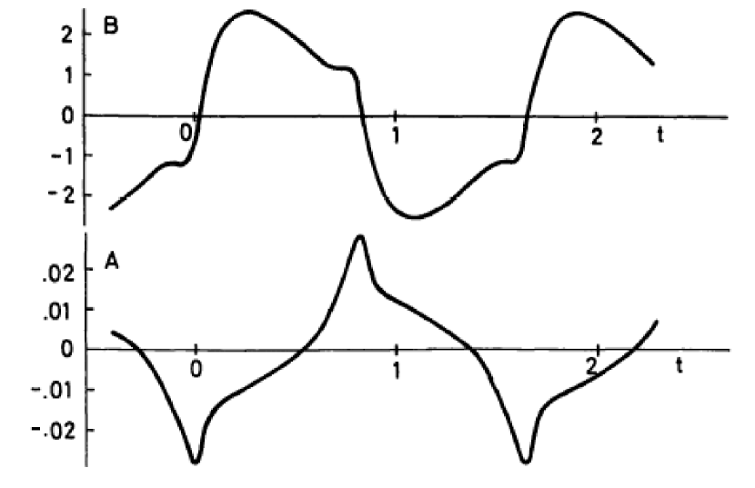
Figure 12: Evolution of toroidal and poloidal fields, $B$ and $A$, respectively, from the paper by Stix (1972). Note the similarity in the evolution of his model and that in the direct simulation shown in Fig. 10, with a more spiky behavior of the poloidal field compared to the toroidal field. [Adapted from Stix (1972).]

4.2 Dynamical $\alpha$ quenching

The $\alpha$ effect formalism provides so far the only workable mathematical framework for describing the large scale dynamo action seen in simulations of helically forced turbulence. The governing equation for the mean magnetic field is

$${\partial\overline{\vec{B}}\over\partial t}=\mbox{\boldmath$\nabla$}{}\times\left(\overline{\vec{U}}\times\overline{\vec{B}}+\overline{\vec{\cal E}}-\eta\mu_{0}\overline{\vec{J}}\right),$$ (17)

where $\overline{\vec{\cal E}}=\overline{{\vec{u}}\times{\vec{b}}}$ is the electromotive force resulting from the ${\vec{u}}\times{\vec{b}}$ nonlinearity in the averaged Ohm’s law. MTA can be used to derive an expression for $\overline{\vec{\cal E}}$ in terms of the mean field. For slow rotation one finds (Rädler et al. 2003, see also review by Brandenburg & Subramanian 2004)

$$\overline{\cal E}_{i}=\alpha_{ij}\overline{B}_{j}-\eta_{ij}\overline{J}_{j}+({\vec{\gamma}}\times\overline{\vec{B}}+{\vec{\delta}}\times\overline{\vec{J}})_{i}+\kappa_{ijk}\overline{B}_{j,k},$$ (18)

Under isotropic conditions, or as a means of simplification, one often just writes

$$\overline{\vec{\cal E}}=\alpha\overline{\vec{B}}-\eta_{\rm t}\overline{\vec{J}}$$ (19)

In any case, and this comes as a rather recent realization (Field & Blackman 2002, Blackman & Brandenburg 2002, Subramanian 2002), there will be an extra magnetic contribution to the $\alpha$ effect $\alpha\to\alpha=\alpha_{\rm K}+\alpha_{\rm M}$. In the isotropic case, $\alpha_{\rm K}=-{\textstyle{1\over 3}}\tau\overline{\mbox{\boldmath$\omega$}{}\cdot{\vec{u}}}$ and $\alpha_{\rm M}={\textstyle{1\over 3}}\tau\overline{{\vec{j}}\cdot{\vec{b}}}/\rho$. This leads to (Kleeorin & Ruzmaikin 1982; see also Zeldovich et al. 1983; and Kleeorin et al. 1995)

$${{\rm d}{}\alpha_{\rm M}\over{\rm d}{}t}=-2\eta_{\rm t0}k_{\rm f}^{2}\left({\langle\overline{\vec{\cal E}}\cdot\overline{\vec{B}}\rangle\over B_{\rm eq}^{2}}+{\alpha_{\rm M}\over\tilde{R}_{\rm m}}\right),$$ (20)

where we have defined the magnetic Reynolds number as

$$\tilde{R}_{\rm m}=\eta_{\rm t0}/\eta,$$ (21)

where $\eta_{\rm t0}={\textstyle{1\over 3}}\tau\langle{\vec{u}}^{2}\rangle$ is the kinematic value of the turbulent magnetic diffusivity and $B_{\rm eq}^{2}=\mu_{0}\rho_{0}\langle{\vec{u}}^{2}\rangle$ is the equipartition field strength. Equation (20) agrees with the corresponding equation in Kleeorin et al. (1995) if their characteristic length scale of the turbulent motions at the surface, $l_{\rm s}$, is identified with $2\pi/k_{\rm f}$ and if their parameter $\mu$ is identified with $8\pi^{2}\eta_{\rm t0}^{2}/(\langle{\vec{u}}^{2}\rangle l_{\rm s}^{2})$. The definition of $\tilde{R}_{\rm m}$ may not be very practical if $\eta_{\rm t0}$ is not known, but comparison with simulations (Blackman & Brandenburg 2002) suggests that $\tilde{R}_{\rm m}\approx 0.3R_{\rm m}$, where $R_{\rm m}=u_{\rm rms}/(\eta k_{\rm f})$ is a more practical definition suitable for simulations of forced turbulence.

The basic idea is that magnetic helicity conservation must be obeyed, but the presence of an $\alpha$ effect leads to magnetic helicity of the mean field which has to be balanced by magnetic helicity of the fluctuating field. This magnetic helicity of the fluctuating (small scale) field must be of opposite sign to that of the mean (large scale) field (e.g. Blackman & Brandenburg 2003). In the following we refer to Eq. (20) as the the dynamical $\alpha$ quenching equation (Blackman & Brandenburg 2002). Assuming that the large scale magnetic field has reached a steady state, and solving this equation for $\alpha$, yields (Kleeorin & Ruzmaikin 1982, Gruzinov & Diamond 1994)

$$\alpha={\alpha_{\rm K}+\eta_{\rm t}R_{\rm m}\langle\overline{\vec{J}}\cdot\overline{\vec{B}}\rangle/B_{\rm eq}^{2}\over 1+R_{\rm m}\langle\overline{\vec{B}}^{2}\rangle/B_{\rm eq}^{2}}\quad\mbox{(for ${\rm d}{}\alpha/{\rm d}{}t=0$)}.$$ (22)

Note that for the numerical experiments with an imposed large scale field over the scale of the box (Cattaneo & Hughes 1996), where $\overline{\vec{B}}$ is spatially uniform and therefore $\overline{\vec{J}}=0$, one recovers the ‘catastrophic’ quenching formula,

$$\alpha={\alpha_{\rm K}\over 1+R_{\rm m}\langle\overline{\vec{B}}^{2}\rangle/B_{\rm eq}^{2}}\quad\mbox{(for $\overline{\vec{J}}=0$)},$$ (23)

which implies that $\alpha$ becomes quenched when $\langle\overline{\vec{B}}^{2}\rangle/B_{\rm eq}^{2}=R_{\rm m}^{-1}\approx 10^{-8}$ for the sun, and for even smaller fields in the case of galaxies.

Obviously, the assumption of a steady state is generally not permitted. Especially in the case of closed boxes that are so popular for simulation purposes, there is no other way to get rid of magnetic helicity than via microscopic resistivity. There is now a significant body of literature (see Brandenburg 2001 for a comprehensive coverage of the simulation results and Brandenburg 2003 for a recent review). To allow for faster time scales, and this was realized first by Blackman & Field (2000a,b) and Kleeorin et al. (2000), there might be hope to achieve this by allowing helicity flux to escape through the boundaries of the domain. Two types of results will be discussed in the next section.

5 Open boundaries and shear: the solution?

In a recent paper, Brandenburg & Sandin (2004) have carried out a range of simulations for different values of the magnetic Reynolds number, $R_{\rm m}=u_{\rm rms}/(\eta k_{\rm f})$, for both open and closed boundary conditions using the geometry depicted in Fig. 13. In the following we discuss first some results for $\alpha$ quenching and an interpretation of the results in terms of the current helicity flux. Next we turn to direct simulations of the dynamo without an imposed field.

5.1 Results for $\alpha$ quenching

In order to measure $\alpha$, a uniform magnetic field, ${\vec{B}}_{0}={\rm const}{}$, is imposed, and the magnetic field is now written as ${\vec{B}}={\vec{B}}_{0}+\mbox{\boldmath$\nabla$}{}\times{\vec{A}}$. Brandenburg & Sandin (2004) determined $\alpha$ by measuring the turbulent electromotive force, and hence $\alpha=\langle\mbox{\boldmath${\cal E}$}{}\rangle\cdot{\vec{B}}_{0}/B_{0}^{2}$. Similar investigations have been done before both for forced turbulence (Cattaneo & Hughes 1996, Brandenburg 2001) and for convective turbulence (Brandenburg et al. 1990, Ossendrijver et al. 2001).

As expected, $\alpha$ is negative when the helicity of the forcing is positive, and $\alpha$ changes sign when the helicity of the forcing changes sign. The magnitudes of $\alpha$ are however different in the two cases: $|\alpha|$ is larger when the helicity of the forcing is negative. In the sun, this corresponds to the sign of helicity in the northern hemisphere in the upper parts of the convection zone. This is here the relevant case, because the differential rotation pattern of the present model also corresponds to the northern hemisphere.

Figure 13: Differential rotation in our cartesian model, with the equator being at the bottom, the surface to the right, the bottom of the convection zone to the left and mid-latitudes at the top. [Adapted from Brandenburg & Sandin (2004).]

There is a striking difference between the cases with open and closed boundaries which becomes particularly clear when comparing the averaged values of $\alpha$ for different magnetic Reynolds numbers; see Fig. 14. With closed boundaries $\alpha$ tends to zero like $R_{\rm m}^{-1}$, while with open boundaries $\alpha$ shows no such decline. There is also a clear difference between the cases with and without shear together with open boundaries in both cases. In the absence of shear (dotted line in Fig. 14) $\alpha$ declines with increasing $R_{\rm m}$, even though for small values of $R_{\rm m}$ it is larger than with shear. The difference between open and closed boundaries will now be discussed in terms of a current helicity flux through the two open boundaries of the domain.

Figure 14: Dependence of $|\langle\alpha\rangle|/u_{\rm rms}$ on $R_{\rm m}$ for open and closed boundaries. The case with open boundaries and negative helicity is shown as a dashed line. Note that for $R_{\rm m}\approx 30$ the $\alpha$ effect is about 30 times smaller when the boundaries are closed. The dotted line gives the result with open boundaries but no shear. The vertical lines indicate the range obtained by calculating $\alpha$ using only the first and second half of the time interval. [Adapted from Brandenburg & Sandin (2004).]

5.2 Interpretation in terms of current helicity flux

It is suggestive to interpret the above results in terms of the dynamical $\alpha$ quenching model. However, the quenching equation has to be generalized to take the divergence of the flux into account. In order to avoid problems with the gauge, it is advantageous to work directly with $\overline{{\vec{j}}\cdot{\vec{b}}}$ instead of $\overline{{\vec{a}}\cdot{\vec{b}}}$. Using the evolution equation, $\partial{\vec{b}}/\partial t=-\mbox{\boldmath$\nabla$}{}\times\mbox{\boldmath$e$}{}$, for the fluctuating magnetic field, where $\mbox{\boldmath$e$}{}={\vec{E}}-\overline{\vec{E}}$ is the small scale electric field and $\overline{\vec{E}}=\eta\mu_{0}\overline{\vec{J}}-\overline{\vec{\cal E}}$ the mean electric field, one can derive the equation

$${\partial\over\partial t}\overline{{\vec{j}}\cdot{\vec{b}}}=-2\,\overline{\mbox{\boldmath$e$}{}\cdot{\vec{c}}}-\mbox{\boldmath$\nabla$}{}\cdot\overline{\mbox{\boldmath${\cal F}$}}{}_{C}^{\rm SS},$$ (24)

where

$$\overline{\mbox{\boldmath${\cal F}$}}{}_{C}^{\rm SS}=\overline{2\mbox{\boldmath$e$}{}\times{\vec{j}}}+\overline{(\mbox{\boldmath$\nabla$}{}\times\mbox{\boldmath$e$}{})\times{\vec{b}}}/\mu_{0},$$ (25)

is the current helicity flux from the small scale (SS) field, and ${\vec{c}}=\mbox{\boldmath$\nabla$}{}\times{\vec{j}}$ the curl of the small scale current density, ${\vec{j}}={\vec{J}}-\overline{\vec{J}}$. In the isotropic case, $\overline{\mbox{\boldmath$e$}{}\cdot{\vec{c}}}\approx k_{\rm f}^{2}\overline{\mbox{\boldmath$e$}{}\cdot{\vec{b}}}$, where $k_{\rm f}$ is the typical wavenumber of the fluctuations, here assumed to be the forcing wavenumber.

Making use of the adiabatic approximation one arrives at the algebraic steady state quenching formula ($\partial\alpha/\partial t=0$)

$$\alpha={\alpha_{\rm K}+R_{\rm m}\left(\eta_{\rm t}\mu_{0}\overline{\vec{J}}\cdot\overline{\vec{B}}-{\textstyle{1\over 2}}k_{\rm f}^{-2}\mbox{\boldmath$\nabla$}{}\cdot\mu_{0}\overline{\mbox{\boldmath${\cal F}$}}{}_{C}^{\rm SS}\right)/B_{\rm eq}^{2}\over 1+R_{\rm m}\overline{\vec{B}}^{2}/B_{\rm eq}^{2}}.$$ (26)

In the absence of a mean current, e.g. if the mean field is defined as an average over the whole box, then $\overline{\vec{B}}\equiv{\vec{B}}_{0}={\rm const}{}$, and $\overline{\vec{J}}=0$, so Eq. (26) reduces to

$$\alpha={\alpha_{\rm K}-{\textstyle{1\over 2}}k_{\rm f}^{-2}R_{\rm m}\mbox{\boldmath$\nabla$}{}\cdot\mu_{0}\overline{\mbox{\boldmath${\cal F}$}}{}_{C}^{\rm SS}/B_{\rm eq}^{2}\over 1+R_{\rm m}{\vec{B}}_{0}^{2}/B_{\rm eq}^{2}}.$$ (27)

This expression applies to the present case, because we consider only the statistically steady state and we also define the mean field as a volume average.

In the simulations, the current helicity flux is found to be independent of the magnetic Reynolds number. This explains why the $\alpha$ effect no longer shows the catastrophic $R_{\rm m}^{-1}$ dependence (see Fig. 14). In principle it is even conceivable that with $\alpha_{\rm K}=0$ a current helicity flux can be generated, for example by shear, and that this flux divergence could drive a dynamo, as was suggested by Vishniac & Cho (2001). It is clear, however, that for finite values of $R_{\rm m}$ this would be a non-kinematic effect requiring the presence of an already finite field (at least of the order of $B_{\rm eq}/R_{\rm m}^{1/2}$). This is because of the $1+R_{\rm m}{\vec{B}}_{0}^{2}/B_{\rm eq}^{2}$ term in the denominator of Eq. (27). At the moment we cannot say whether this is perhaps the effect leading to the nonhelically forced turbulent dynamo discussed in Sect. 5.3, or whether it is perhaps the ${\vec{\delta}}\times\overline{\vec{J}}$ or shear-current effect that was also mentioned in that section.

5.3 Dynamos with open surfaces and shear

The presence of an outer surface is in many respects similar to the presence of an equator. In both cases one expects magnetic and current helicity fluxes via the divergence term. A particularly instructive system is helical turbulence in an infinitely extended horizontal slab with stress-free boundary conditions and a vertical field condition, i.e.

$$u_{x,z}=u_{y,z}=u_{z}=B_{x}=B_{y}=0.$$ (28)

Without shear, such simulations have been performed by Brandenburg & Dobler (2001) who found that a mean magnetic field is generated, similar to the case with periodic boundary conditions, but that the energy of the mean magnetic field, $\langle\overline{\vec{B}}^{2}\rangle$, decreases with magnetic Reynolds number. Nevertheless, the energy of the total magnetic field, $\langle{\vec{B}}^{2}\rangle$, does not decrease with increasing magnetic Reynolds number. Although they found that $\langle\overline{\vec{B}}^{2}\rangle$ decreases only like $R_{\rm m}^{-1/2}$, new simulations confirm that a proper scaling regime has not yet been reached and that the current data may well be compatible with an $R_{\rm m}^{-1}$ dependence.

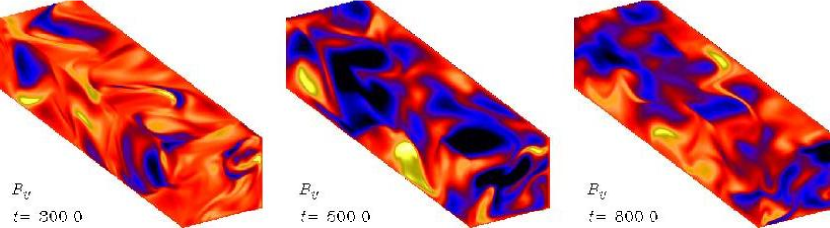
Figure 15: Visualization of the toroidal magnetic field during three different times during the growth and saturation for the run without kinetic helicity.

Clearly, an asymptotic decrease of the mean magnetic field must mean that the small scale dynamo does not work with such boundary conditions. Thus, the anticipated advantages of open boundary conditions are not borne out by this type of simulations. In the presence of shear the results are very different. We now use the same setup as in Sect. 5.1. The size of the computational domain is ${\textstyle{1\over 2}}\pi\times 2\pi\times{\textstyle{1\over 2}}\pi$ and the numerical resolution is $128\times 512\times 128$ meshpoints. The magnetic Reynolds number based on the forcing wavenumber and the turbulent flow is around 80 and shear flow velocity exceeds the rms turbulent velocity by a factor of about 5. We have carried out experiments with no helicity in the forcing (labeled as $\alpha=0$), as well as positive and negative helicity in the forcing (labeled $\alpha<0$ and $\alpha>0$, respectively); see Fig. 15 for a visualization of the run without kinetic helicity. We emphasize that no explicit $\alpha$ effect has been invoked. The labeling just reflects the fact that, in isotropic turbulence, negative kinetic helicity (as in the northern hemisphere of a star or the upper disc plane in galaxies) leads to a positive $\alpha$ effect, and vice versa.

Figure 16: Saturation behavior of the ratio $q=\langle\overline{\vec{B}}^{2}\rangle/\langle{\vec{B}}^{2}\rangle$ for runs with different kinetic helicity of the flow. Solid line: zero helicity, dotted line: positive helicity (opposite to the sun) dashed line: negative helicity (as in the sun). The line at denoted by “$\alpha=0$, closed” refers to a case where the normal field condition on the equator and the surface has been replaced by a perfect conductor condition.

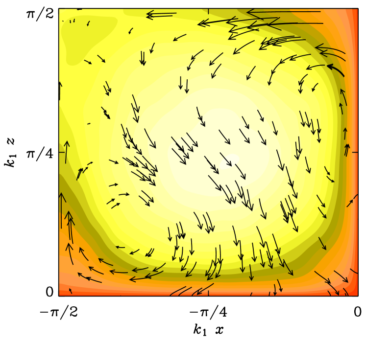
Figure 17: Gray/color scale representation of the azimuthally and time averaged mean azimuthal field $\overline{\vec{B}}$ together with vectors in the meridional plane. In this run the turbulence is nonhelically forced ($\alpha=0$).

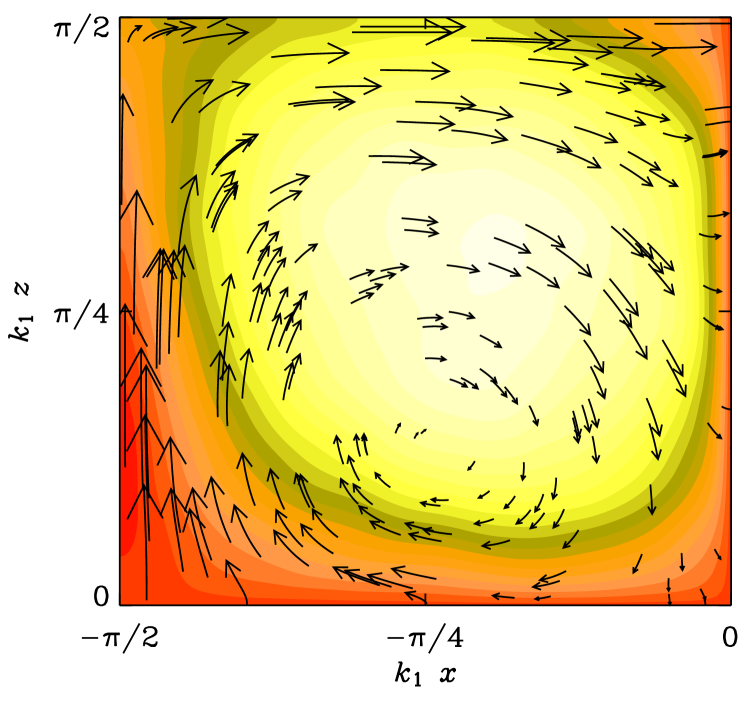
Figure 18: Same as Fig. 17, but for $\alpha>0$, so the turbulence is forced with negative helicity. Note the clockwise sense of the poloidal field. Together with the positive toroidal field (indicated by light shades) this corresponds to positive magnetic helicity, consistent with $\alpha>0$.

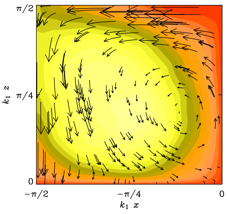
Figure 19: Same as Fig. 17, but for $\alpha<0$, so the turbulence is forced with positive helicity. Note the anti-clockwise sense of the poloidal field, corresponding to negative magnetic helicity, consistent with $\alpha>0$.

Figure 20: Vectors of $\phi_{iyy}$ together with contours of $\overline{U}_{y}$ which also coincide with the streamlines of the mean vorticity field $\overline{\vec{W}}$. Note the close agreement between $\phi_{iyy}$ and $\overline{\vec{W}}$. The orientation of the vectors indicates that negative current helicity leaves the system at the outer surface ($x=0$).

We characterize the relative strength of the mean field by the ratio $q=\langle\overline{\vec{B}}^{2}\rangle/\langle{\vec{B}}^{2}\rangle$, where overbars denote an average in the toroidal ($y$) direction; see Fig. 16. A strong mean field is generated in all cases, unless a perfect conductor boundary condition (“closed”) is adopted on the outer surface and on the equator. The mean field appears to be statistically stationary in all cases, i.e. there is no indication of migration in the meridional plane. A time average of the mean field is shown in Fig. 17.

There are two surprising results emerging from this work. First, in the presence of shear rather strong mean fields can be generated, where up to 70% of the energy can be in the mean field; see Fig. 16. Second, even without any kinetic helicity in the flow there is strong large scale field generation. However, this cannot be an $\alpha\Omega$ dynamo in the usual sense. One possibility is the ${\vec{\delta}}\times{\vec{J}}$ effect, which emerged originally in the presence of the Coriolis force; see Rädler (1969) and Krause & Rädler (1980). In the present case with no Coriolis force, however, a ${\vec{\delta}}\times{\vec{J}}$ effect is possible even in the presence of shear alone, because the vorticity associated with the shear contributes directly to ${\vec{\delta}}\propto\overline{\vec{W}}=\mbox{\boldmath$\nabla$}{}\times\overline{\vec{U}}$ (Rogachevskii & Kleeorin 2003, 2004).

A rather likely candidate for the current helicity flux is the so-called Vishniac & Cho (2001) flux. A systematic derivation using MTA (Subramanian & Brandenburg 2004) gave

$$\overline{\cal F}^{\rm SS}_{C\,i}=\phi_{ijk}\overline{B}_{j}\overline{B}_{k},$$ (29)

where $\phi_{ijk}$ is a new turbulent transport tensor with

$$\phi_{ijk}=-4\tau\overline{\omega_{k}\nabla_{j}u_{i}}.$$ (30)

Obviously, only components of $\phi_{ijk}$ that are symmetric in $j$ and $k$ enter the flux $\overline{\mbox{\boldmath${\cal F}$}}{}_{C}^{\rm SS}$. Therefore we consider in the following $\phi_{ijk}^{\rm S}={\textstyle{1\over 2}}(\phi_{ijk}+\phi_{ikj})$. In the present case where the toroidal field ($y$ direction) is strongest, the $\phi_{iyy}$ components (where $i=x$ and $z$) are expected to be most important. The time average of this component is shown in Fig. 20. Here we have only considered the nonhelical case, but the helical cases are indistinguishable within error margins. All the 6 independent components of $\phi_{xij}^{\rm S}$ and $\phi_{zjk}^{\rm S}$ are given by

$$\phi_{xjk}^{\rm S}=\pmatrix{-0.03&+0.04&-0.12\cr+0.04&-0.23&-0.36\cr-0.12&-0.36&+0.25},$$ (31)

$$\phi_{zjk}^{\rm S}=\pmatrix{+0.24&+0.32&-0.13\cr+0.32&-0.19&-0.05\cr-0.13&-0.05&-0.04}.$$ (32)

Note that the trace of both tensors is small. Thus there is no hope that this tensor could possibly be isotropic. This is because isotropization, i.e. ${\textstyle{1\over 3}}\delta_{jk}\phi_{ijk}$, would then give something close to zero. Nevertheless, one may hope that some useful parameterization of $\phi_{ijk}^{\rm S}$, that can be used in mean field calculations, will soon be available.

In conclusion, there is evidence that the strong dynamo action seen in the simulations is only possible due to the combined presence of open boundaries and shear.

6 Conclusions

In the present work we have discussed three aspects that are strongly connected with the applicability of mean field dynamo theory. The first concerns turbulent diffusion, i.e. the ability of the flow to mix a large scale magnetic field such that its energy can be converted into energy at smaller scales. In order that microscopic diffusion can eventually be thermalized, unimpeded by the Lorentz force, the field has to be weak enough at the scale where diffusion takes place. Whether this is indeed the case can in principle be seen from the simulations. Since in the simulations the magnetic and fluid Reynolds numbers are much smaller than in reality, it would be important to show that the spectra begin to converge for large magnetic and fluid Reynolds numbers. At the moment this is simply not yet the case, even at a resolution of $1024^{3}$ meshpoints. However, by a combination between direct and large eddy simulations some preliminary insight can be gained. The suggestions are that magnetic and kinetic energy spectra approach spectral equipartition in the deep inertial range, and that the slope would be comparable to the Kolmogorov $k^{-5/3}$ slope.

The other aspect discussed in this paper concerns the calculation of turbulent transport coefficients such as the $\alpha$ effect. It has been particularly disturbing that much of the theory in this field was based on the first order smoothing approximation which clearly should break down under physically interesting conditions. The reason for its apparent success is now becoming clear and are connected with the close similarity between the first order smoothing approximation and the minimal tau approximation where the triple correlations are no longer omitted. The reason for the close similarity between the two approaches is mainly connected with the fact that all the interesting physics enters via the quadratic correlations which can be worked out correctly using linear theory. The significance of the triple correlations is merely that they determine the length of $\tau$. In the framework of the first order smoothing approximation the value of $\tau$ had to be obtained by dimensional arguments and was therefore not well determined.

Next we have briefly addressed the long standing issue of $\alpha$ quenching and have pointed out the connection between dynamical quenching and catastrophic quenching. The possibility of catastrophic $\alpha$ quenching is closely linked to magnetic helicity conservation. The degree of quenching can therefore be alleviated by allowing for magnetic or better current helicity fluxes. Such fluxes do not just come on their own, so simply allowing for the boundaries to be open is not sufficient. One needs to drive a flux through the entire domain. This seems to be accomplished by the Vishniac-Cho flux. As already argued by Vishniac & Cho (2001), and confirmed by Arlt & Brandenburg (2001), this flux can be driven in the presence of shear. Indeed, there are strong indications that the helicity flux can alleviate catastrophic quenching at least by a factor of about 30, and that it allows for dynamo action generating strong magnetic fields, even in the absence of helicity in the forcing. The details of this process are not entirely clear, but possible candidates include the shear-current effect of Rogachevskii & Kleeorin (2003, 2004), and perhaps the helicity flux itself (Vishniac & Cho 2001) which is a nonlinear effect.

In the near future it should be possible to investigate the emergence of current helicity fluxes from a dynamo simulation in more detail. This would be particularly interesting in view of the many observations of coronal mass ejections that are known to be associated with significant losses of magnetic helicity and hence also of current helicity (Berger & Ruzmaikin 2000, DeVore 2000, Chae 2000, Low 2001, Démoulin et al. 2002, Gibson et al. 2002). In order to be able to model coronal mass ejections it should be particularly important to relax the restrictions imposed by the vertical field conditions employed in the simulations of Brandenburg & Sandin (2004). One possibility would be to include a simplified version of a corona with enhanced temperature and hence decreased density, giving rise to a low-beta plasma exterior where nearly force-free fields can develop (Gudiksen & Nordlund 2003). Such a setup might allow detailed comparison with observations.