Shearing and embedding box simulations of the magnetorotational instability

Abstract

Two different computational approaches to the magnetorotational instability (MRI) are pursued: the shearing box approach which is suited for local simulations and the embedding box approach whereby a Taylor Couette flow is embedded in a box so that numerical problems with the coordinate singularity are avoided. New shearing box simulations are presented and differences between regular and hyperviscosity are discussed. Preliminary simulations of spherical nonlinear Taylor Couette flow in an embedding box are presented and the effects of an axial field on the background flow are studied.

1 Introduction

It is now generally accepted that the magnetorotational instability (MRI) is the main agent driving turbulence in accretion discs Balbus and Hawley (1998). This instability provides a good explanation for the turbulence in accretion discs which might otherwise be hydrodynamically stable Balbus et al. (1996). The historical developments of the understanding of this instability have appropriately been reviewed elsewhere in this book. Here we focus mainly on results within the shearing sheet approximation, which is the relevant extension of a periodic geometry to a shearing environment. Like with periodic “boundary” conditions, there is actually no boundary, and every point in the domain is equivalent to any other point. This avoids boundary layers which is extremely useful for simulations, but it is also astrophysically more relevant because we do not want explicit boundaries in a local domain that is supposed to represent a subvolume within the global disc. In the following we present a discussion of the nonaxisymmetric MRI in the shearing sheet approximation using the Rayleigh quotient to define in a convenient way an “instantaneous” growth rate of otherwise only transient growth. In this paper we also calculate the nonlinear evolution of the MRI, reviewing both old simulations using subgrid scale modeling and new direct simulations where the ordinary viscosity and diffusion operators are used with uniform coefficients. Finally we turn to the issue of spherical Couette flow and present preliminary simulations in order to address recent experimental results suggestive of MRI in liquid sodium.

2 Axisymmetric vs nonaxisymmetric MRI

In order to obtain the dispersion relation for the MRI with a vertical magnetic field it suffices to consider the linearized pressureless one-dimensional momentum equation and the linearized induction equation for the two components in the rotational ($x,y$) plane, i.e.

$$\dot{u}_{x}-2\Omega u_{y}^{\prime}=v_{\rm A}b_{x}^{\prime},$$ (1)

$$\dot{u}_{y}+(2-q)\Omega u_{x}^{\prime}=v_{\rm A}b_{y}^{\prime},$$ (2)

$$\dot{b}_{x}=v_{\rm A}b_{x}^{\prime},$$ (3)

$$\dot{b}_{y}+q\Omega b_{x}^{\prime}=v_{\rm A}b_{y}^{\prime},$$ (4)

where dots and primes denote derivatives with respect to $t$ and $z$, respectively, $u$ and $b$ are linearized velocity and magnetic field, and $q$ denotes the steepness of the rotation law with $\Omega\sim R^{-q}$ where $q=3/2$ for purely keplerian discs. In our local cartesian model, $y$ is the streamwise direction and $x$ is the cross-stream direction.

One could have retained the $u_{z}$ component of the momentum equation where the pressure gradient would enter, together with the continuity equation, but these two equations decouple from those considered already. The resulting new modes are the fast magnetosonic waves, which are of no particular interest in the present context.

Assuming that the solution is proportional to $e^{{\rm i}kz-{\rm i}\omega t}$, we obtain the dispersion relation Balbus and Hawley (1991, 1998) in the form

$$\omega^{4}-2\omega^{2}\left[v_{A}^{2}k^{2}+(2-q)\Omega^{2}\right]+v_{A}^{2}k^{2}\left(v_{A}^{2}k^{2}-2q\Omega^{2}\right)=0.$$ (5)

This is a bi-quadratic equation with altogether 4 solutions, corresponding to two different branches where $\omega$ can have either sign on each of them. The two branches are

$$\omega_{\pm}^{2}=v_{A}^{2}k^{2}+(2-q)\Omega^{2}\pm\Omega\sqrt{4v_{A}^{2}k^{2}+(2-q)^{2}\Omega^{2}}.$$ (6)

The upper branch corresponds to Alfvén waves and the lower branch corresponds to slow magnetosonic waves. The fast magnetosonic waves have been eliminated by using the pressureless momentum equation. In the range $0<v_{\rm A}^{2}k^{2}<3$ the slow magnetosonic waves can become unstable, i.e. $\omega_{-}^{2}<0$, corresponding to an exponentially growing solution with growth rate $\mbox{Im}\,\omega_{-}$. The maximum growth rate is reached when $v_{A}^{2}k^{2}={15\over 16}\Omega^{2}$, and the corresponding value of $\omega_{-}^{2}$ is then $\mbox{Im}\,\omega_{-}={3\over 4}\Omega$; see Fig. 1.

Figure 1: Solutions of the dispersion relation (6) for accretion disc parameters ($q=3/2$, thick solid lines), compared with the dispersion relation for a rigidly rotating disc ($q=0$, dotted lines) and an almost nonrotating disc ($q=0$ and $\Omega=0.01\Omega_{0}$, dashed lines). Here, $\Omega_{0}^{2}=GM/R^{3}$ is the keplerian value at radius $R$. The upper set of curves denotes Alfvén waves and the lower set slow magnetosonic waves. Note that in the completely nonrotating case ($\Omega=0$) the Alfvén and slow magnetosonic waves are degenerate.

In the nonaxisymmetric case the situation is not quite as simple, because now $\partial/\partial y\neq 0$, and this leads to the occurrence of a new term with a non-constant coefficient. This comes from the $\overline{\bf{U}}\cdot{\bm{\nabla}}$ advection terms in all four equations, because $\overline{\bf{U}}=Sx\hat{\bm{y}}$. There are two different ways of dealing with this problem. One possibility is to abandon the assumption of harmonic solutions in the $x$ direction, i.e. one assumes ${\bm{u}}=\hat{{\bm{u}}}(x)e^{{\rm i}k_{y}y+{\rm i}k_{z}z-{\rm i}\omega t}$. This approach has been taken by Ogilvie and Pringle (1996), for example. Another possibility is to assume shearing-periodic boundary conditions. The way then to get rid of the $x$ dependence in the $Sx\partial/\partial y$ term is by assuming $k_{x}$ to depend on time, because then the $\partial/\partial t$ term pulls down a factor $\dot{k}_{x}x$ that can be arranged such as to cancel the $Sxk_{y}$ term that results from the $Sx\partial/\partial y$ term. (Here, as before, the dots denote a derivative with respect to $t$.) This requires $\dot{k}_{x}x+Sxk_{y}=0$, i.e.

$$k_{x}(t)=k_{x0}-Stk_{y},$$ (7)

where $k_{x0}$ is some initial values of $k_{x}$. Using the ansatz

$${\bm{q}}(x,y,z,t)=A\,\mbox{Re}\,\hat{{\bm{q}}}(t)\,\exp\left[{\rm i}k_{x}(t)x+{\rm i}k_{y}y+{\rm i}k_{z}z\right],$$ (8)

where the hats denote the shearing sheet expansion, $A$ is an amplitude factor, and $\hat{{\bm{q}}}=(\hat{u}_{x},\hat{u}_{y},\hat{u}_{z},\hat{b}_{x},\hat{b}_{y},\hat{b}_{z},\hat{\Lambda})^{T}$ is the state vector with $\Lambda=c_{\rm s}\ln\rho$, ${\bm{b}}={\bm{B}}/\sqrt{\mu_{0}\rho_{0}}$, the partial differential equation

$${\rm i}{\partial{\bm{q}}\over\partial t}+{\rm i}Sx{\partial{\bm{q}}\over\partial y}={\sf{\bm{L}}}{\bm{q}},$$ (9)

with non-constant coefficients, turns into an ordinary differential equation with constant coefficients Goldreich and Lynden-Bell (1965); Balbus and Hawley (1992a),

$${\rm i}{{\rm d}{}\hat{{\bm{q}}}\over{\rm d}{}t}=\hat{{\sf{\bm{L}}}}\hat{{\bm{q}}}.$$ (10)

Without going into the details of the derivation we simply state the governing matrix, $\hat{{\sf{\bm{L}}}}$, for the case with uniform density $\rho_{0}$, a uniform magnetic field in the $y$ direction, $\hat{\bm{y}}B_{0}$, and Alfvén speed $v_{\rm A}=B_{0}/\sqrt{\mu_{0}\rho_{0}}$ and an isothermal equation of state,

$$\hat{{\sf{\bm{L}}}}=\pmatrix{0&2{\rm i}\Omega&0&-k^{\rm A}_{y}&k^{\rm A}_{x}&0&k^{\rm c}_{x}\cr-2{\rm i}\Omega^{\rm S}&0&0&0&0&0&k^{\rm c}_{y}\cr 0&0&0&0&k^{\rm A}_{z}&-k^{\rm A}_{y}&k^{\rm c}_{z}\cr-k^{\rm A}_{y}&0&0&0&0&0&0\cr k^{\rm A}_{x}&0&k^{\rm A}_{z}&{\rm i}S&0&0&0\cr 0&0&-k^{\rm A}_{y}&0&0&0&0\cr k^{\rm c}_{x}&k^{\rm c}_{y}&k^{\rm c}_{z}&0&0&0&0}\!,$$ (11)

where we have used the abbreviations $2\Omega^{\rm S}=2\Omega+S$, $k^{\rm A}_{i}=k_{i}v_{\rm A}$, $k^{\rm c}_{i}=k_{i}c_{\rm s}$. In the stratified case with a uniform background field, the system of governing equations has variable coefficients. Therefore we only consider here the case of constant density. Note that $\hat{{\sf{\bm{L}}}}$ is hermitian if $S=0$. This property ensures that all eigenvalue are stable in that case.

The set of equations (10) were already investigated by Balbus and Hawley (1992a) using numerical integration. They looked at the evolution $\hat{{\bm{q}}}$ and found a transient behavior that depends on initial conditions. Foglizzo and Tagger (1994, 1995) studied the nonaxisymmetric stability in the presence of density stratification which also gives rise to the Parker instability. A convenient method to calculate the growth rates of the MRI is in terms of the Rayleigh quotient (see Brandenburg and Dintrans (2001))

$$\omega(t)={\langle\hat{{\bm{q}}}|\hat{{\sf{\bm{L}}}}\hat{{\bm{q}}}\rangle\over\langle\hat{{\bm{q}}}|\hat{{\bm{q}}}\rangle},$$ (12)

where $\displaystyle\langle{\bm{a}}|{\bm{b}}\rangle=\sum_{i=1}^{N}a^{*}_{i}b_{i}$ defines a scalar product. To ensure solenoidality of the magnetic field, we calculate $\hat{b}_{x}$ for the initial perturbation from Balbus and Hawley (1992a)

$$\hat{b}_{x}(0)=-(k_{y}\hat{b}_{y}+k_{z}\hat{b}_{z})/k_{x0}.$$ (13)

The results for the keplerian case, $S/\Omega=-3/2$, are shown in Figs 2 and 3. In agreement with earlier work Balbus and Hawley (1992a); Kim and Ostriker (2000), the maximum growth rate agrees with the Oort $A$-value Balbus and Hawley (1992b), which is $-S/2$, or ${3\over 4}\Omega$ for keplerian rotation; see also Fig. 1.

Figure 2: Evolution of the imaginary part of $\omega$ (a) and the norm of ${\bm{q}}$ (b) for $v_{\rm A}k_{y}/\Omega=1$. Note that transient amplification is only possible during the time interval when $|v_{\rm A}k_{x}(t)|/\Omega 10$.

Figure 3: Growth rates as a function of Alfvén speed, in units of $\Omega/k_{\parallel}$ where $k_{\parallel}$ denotes $k_{y}$ in the nonaxisymmetric case and $k_{z}$ in the axisymmetric one. Symbols mark the results obtained from the Rayleigh quotient method for the nonaxisymmetric instability with $k_{y}=[0.8,1.2]$. For $v_{\rm A}k_{y}/\Omega>1.7$ our technique fails to yield reliable values of $\omega$ and the noisy oscillations seen in Fig. 2 become dominant. The solid lines indicates the result for the axisymmetric MRI (Eq. 6).

Figure 4: Transient amplification of the magnetic field by the nonaxisymmetric magnetorotational instability. The solid line shows the result from the Rayleigh quotient method while the broken lines give the result from direct three-dimensional simulations with zero viscosity and zero resistivity. The square root of the Rayleigh quotient has been scaled by a factor $c_{q}=3.5\times 10^{-5}$ to make it overlap with $B_{\rm rms}$ curve. A resolution of only $32^{3}$ meshpoints is completely insufficient to resolve even the beginning of the instability. At least $256^{3}$ meshpoints are required to resolve the maximum. After $\Omega t>17$ even the simulation with $256^{3}$ meshpoints becomes under-resolved.

Thus, we see that in the nonaxisymmetric case the MRI shows great similarity with the axisymmetric counterpart. However, in the present case of the shearing sheet approximation it is strictly speaking only a transient. This becomes more obvious when looking at the evolution of $\langle{\bm{q}}|{\bm{q}}\rangle^{1/2}$; see Fig. 4 where we see an increase over about three orders of magnitude. In this figure we also show the resulting evolution of the root-mean-square magnetic field from a direct simulation of the shearing sheet equations, where we also adopt an isothermal gas with constant sound speed. The continuity equation is written in terms of the logarithmic density, $\Lambda\equiv\ln\rho$,

$${{\cal D}{}\Lambda\over{\cal D}{}t}=-{\bm{u}}\cdot{\bm{\nabla}}\Lambda-{\bm{\nabla}}\cdot{\bm{u}},$$ (14)

and the induction equation is solved in terms of the magnetic vector potential ${\bm{A}}$, where ${\bm{B}}={\bm{\nabla}}\times{\bm{A}}$, and

$${{\cal D}{}{\bm{A}}\over{\cal D}{}t}={\bm{u}}\times{\bm{B}}+{\textstyle{3\over 2}}\Omega_{0}A_{y}\hat{x}+\eta\nabla^{2}{\bm{A}},$$ (15)

$\eta$ being the magnetic diffusivity and $\Omega_{0}$ being the background rotation at the reference radius (the derivation of the shear term in this form is given in Brandenburg et al. (1995)). The momentum equation is solved in the form

$${{\cal D}{}{\bm{u}}\over{\cal D}{}t}=-{\bm{u}}\cdot{\bm{\nabla}}{\bm{u}}-c_{\rm s}^{2}{\bm{\nabla}}\Lambda+{{\bm{J}}\times{\bm{B}}\over\rho}+{\bm{F}}_{\rm visc}+\mbox{\boldmath$f$}{},$$ (16)

where ${\cal D}{}/{\cal D}{}t=\partial/\partial t+u_{y}^{(0)}\frac{\partial}{\partial y}$ and $u_{y}^{(0)}=-(3/2)\Omega_{0}x$ is the velocity in the y-direction due to the shear flow. Furthermore ${\bm{J}}={\bm{\nabla}}\times{\bm{B}}/\mu_{0}$ is the current density, ${\bm{B}}$ is the magnetic field, $\mu_{0}$ is the vacuum permeability and ${\bm{F}}_{\rm visc}$ is the viscous force.

The initial condition for the 3-dimensional direct simulation is obtained by evolving linearized shearing sheet equations for $k_{y}=1$ and $k_{z}=10$ to the point where $k_{x}(t_{0})=-5$. [The size of the domain is $(2\pi)^{3}$.] For definitiveness, we reproduce here the numerical values in equation (8):

$$\hat{{\bm{u}}}=\pmatrix{-0.3108-0.0366{\rm i}\cr-0.4610-0.0542{\rm i}\cr-0.0883-0.0104{\rm i}},\quad\hat{{\bm{b}}}=\pmatrix{+0.0683-0.5813{\rm i}\cr-0.0393+0.3340{\rm i}\cr+0.0347-0.2950{\rm i}},$$ (17)

and the logarithmic density is given by $\hat{\Lambda}=0.042-0.3647{\rm i}$. The amplitude is chosen to be $A=10^{-4}$. Figure 5 shows images of $B_{z}$ on the periphery of the simulation domain. The simulations have been carried out using the Pencil Code which is a high-order finite-difference code (sixth order in space and third order in time) for solving the compressible hydromagnetic equations.

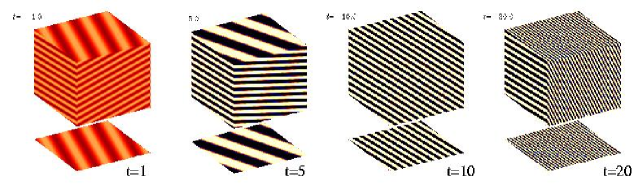
Figure 5: Images of the vertical component of the magnetic field, $B_{z}$, for different values of $t$, where the field at $t=0$ corresponds to that given by equation (17).

The way how this transient amplification can lead to sustained growth is through mode coupling, which is not considered in the present analysis. Relevant mode couplings could come about either through nonuniformities in the cross-stream or $x$ direction and boundary conditions, or through nonlinearities. In the shearing sheet approximation only the latter seems a viable possibility, and this is probably the mechanism through which the early shearing sheet simulations (e.g. Hawley et al. (1995); Matsumoto and Tajima (1995); Brandenburg et al. (1995)) produced sustained turbulence.

3 Local disc simulations and dynamos

The magneto-rotational instability is believed to be of great importance in connection with accretion discs. Here, gas spirals gradually into the center. This is possible mainly because of magnetic stresses, in particular those resulting from the small scale fields, $\overline{b_{r}b_{\phi}}$. They tap potential energy which gets converted into kinetic and magnetic energies, and eventually into heat which gets radiated away. This resistively produced radiation can be so big that it can explain the extreme radiation from quasars that are a hundred times more luminous than ordinary galaxies (e.g. Begelman et al. (1984)).

The standard theory of disc accretion is quite straightforward provided the discs can be treated as geometrically thin (e.g. Frank et al. (1992); Campbell (1997)). The details of the magnetic stress are assumed not to matter. Based on dimensional reasoning the sum of the Reynolds and Maxwell stresses should scale like

$$\left[\overline{u_{r}u_{\phi}}-\overline{b_{r}b_{\phi}}/(\mu_{0}\rho_{0})\right]\approx\alpha_{\rm SS}\Sigma\Omega^{2}H,$$ (18)

where $\alpha_{\rm SS}$ is the magnetic contribution to the dimensionless Shakura-Sunyaev parameter Shakura and Sunyaev (1973), $\Sigma=\int_{0}^{\infty}\rho{\rm d}{}z=2\rho_{0}H$, $\Omega=\sqrt{GM/R^{3}}$ is the keplerian velocity at radius $R$, and $H$ is the scale height. In practice the Maxwell stress is always larger than the Reynolds stress, but both tend to add to the stress, so there is no cancelation. Much of the work on the MRI in discs has focussed on determining the time averaged value of $\alpha_{\rm SS}$. In Fig. 6 we show the evolution of $\alpha_{\rm SS}$ for Run A of Brandenburg et al. (1996).

Figure 6: Comparison of the evolution of $\alpha_{\rm SS}$ (dotted line) with a fit (19) to the mean magnetic field (solid line) using data for Run A of Brandenburg et al. (1996).

Here, much of the time variability comes from the fact that this simulation develops a large scale field, $\overline{\bf{B}}$, that is oscillatory. The dependence $\alpha_{\rm SS}(\overline{\bf{B}})$ can roughly be described via

$$\alpha_{\rm SS}(\overline{\bf{B}})\approx\alpha_{\rm SS}^{(0)}+\alpha_{\rm SS}^{(B)}\overline{\bf{B}}^{2}/B_{0}^{2},$$ (19)

where $\alpha_{\rm SS}^{(0)}\approx 0.002$, $\alpha_{\rm SS}^{(B)}\approx 0.06$, and $B_{0}^{2}=\mu_{0}\langle\rho\rangle\langle c_{\rm s}^{2}\rangle$. In the original simulations of Brandenburg et al. (1995) this time dependence of the large scale field was associated with an $\alpha\Omega$ dynamo. This large scale field also showed migration away from the equatorial plane. Various approaches have subsequently confirmed the initial result that $\alpha$ is negative in the northern hemisphere. This is quite unusual and is probably related to the swirl that comes from the combined action of magnetic buoyancy and the Coriolis force acting on the field-aligned flows driven by the ${\bm{B}}\cdot{\bm{\nabla}}{\bm{B}}$ tension force Brandenburg (1998).

As expected, the dynamo alpha requires the presence of both rotation and stratification. The simulations of Hawley et al. (1996); Stone et al. (1996) without imposed field did show dynamo action, but they assumed periodicity in the vertical direction and there was no net stratification and hence no $\alpha\Omega$ dynamo-type behavior. Subsequent simulations of Miller and Stone (2000) had strong stratification and open boundary conditions. The vertical extent of the box was also much larger than in the previous simulation ($|z|\leq 5H$). Nevertheless, no large scale field was observed. At the moment we can only speculate about the possible origin of this discrepancy. One possibility is the fact that they used a numerical resistivity that allowed very little magnetic helicity to be dissipated. Subsequent work in the context of helically forced turbulence showed that a large scale dynamo effect involving the so-called $\alpha^{2}$ mechanism (for homogeneous helical turbulence, but no shear) can only saturate on a resistive time scale Brandenburg (2001). Whether or not this is indeed the reason for the absence of a large scale field in the simulations of Miller and Stone (2000) remains open.

4 High resolution direct simulations

Several groups have shown independently that the MRI leads to sustained fully three-dimensional turbulence in the presence of an imposed (vertical or toroidal) magnetic field Hawley et al. (1995); Matsumoto and Tajima (1995). Similar simulations have also shown that there is the possibility that the MRI coupled to the dynamo instability can lead to a doubly-positive feedback whereby the dynamo produces the magnetic field for the MRI, which in turn produces the turbulence for the dynamo Brandenburg et al. (1995); Hawley et al. (1996); Stone et al. (1996); Ziegler and Rüdiger (2000).

In all the simulation results published so far, a nonuniform effective viscosity or some other equivalent numerical procedure has been adopted in order to maximize the Reynolds number in regions where the flow is quiescent and to reduce it as much as necessary in regions where the flow shows strong spatial variations. These statements also apply to the effective magnetic diffusivity. Although these procedures are known to provide reasonably safe approximations to many types of turbulent flows Haugen and Brandenburg (2004), there are examples in the context of helical turbulence where departures from the ordinary viscosity and magnetic diffusion operators can lead to major differences compared with the correct solution Brandenburg and Sarson (2002).

In accretion discs the main source of heating is viscous and Joule heating. In the absence of cooling, this would lead to secular heating of the model. In order to avoid this, it is customary to add a volume cooling Brandenburg et al. (1996). In the present model we adopt instead an isothermal gas with constant sound speed. We thus solve equations (14)–(16) using as initial conditions a simple magnetic field configuration given by

$$A_{z}=A_{0}\cos(k_{1}x)\cos(k_{1}y)\cos(k_{1}z),$$ (20)

where $A_{0}=0.2$ has been chosen for all our runs. The initial field strength is chosen rather high so that the wavelength of the most unstable mode, $v_{\rm A}/\Omega$, is large compared with the mesh spacing, $\delta x$. Alternatively, especially for high resolution runs, we use a snapshot from a lower resolution run and remesh it using interpolation.

Unless noted otherwise, we present the results by measuring time in units of $\Omega^{-1}$, length in units of $k_{1}^{-1}$, and density in units of the initial density, $\rho_{0}$. The orbital period is $T_{\rm rot}=2\pi/\Omega$, which is sometimes also used when the time is given as $t/T_{\rm rot}$. We have carried out simulations at three different resolutions with three different viscosities, keeping the magnetic Prandtl number $\mbox{\rm Pr}_{M}=\nu/\eta$ always equal to unity; see Table LABEL:Tsum.

In the run with $128^{3}$ meshpoints we have been able to run for more than three hundred orbital times; see Fig. 7 for a plot showing the evolution of kinetic and magnetic energies. After the first 20 orbits the magnetic energy (per unit volume) decays rapidly and comes then to a halt at around 0.03 (the value quoted in Table LABEL:Tsum).

Table 1: Mean magnetic and kinetic energies (per unit volume and in units of $E_{0}\equiv\rho_{0}\Omega^{2}/k_{1}^{2}$) for runs at different resolution and different viscosities (for unit magnetic Prandtl number, $\nu=\eta$ in units of $\Omega/k_{1}^{2}$). The nondimensional stress is here given as $\tilde{\alpha}_{\rm SS}\equiv[\langle u_{x}u_{y}\rangle-\langle b_{x}b_{y}\rangle/(\mu_{0}\rho_{0})]k_{1}^{2}/\Omega^{2}$. For runs with regular viscosity, the magnetic Reynolds number is defined as $R_{\rm m}=u_{\rm rms}/(\eta k_{1})$. The duration of the run is indicated to give some idea about the statistical significance of the data. In all runs the normalized sound speed is $c_{\rm s}k_{1}/\Omega=5$.

Res. $\nu$ ($=\eta$) $\langle E_{\rm M}\rangle/E_{0}$ $\langle E_{\rm M}\rangle/\langle E_{\rm K}\rangle$ $R_{\rm m}$ $\tilde{\alpha}_{\rm SS}$ $t_{\rm run}/T_{\rm rot}$ status 16 hyp $7.5\times 10^{-5}$ 0.073 3.5 – – 1027 decay 32 hyp $3.5\times 10^{-6}$ 0.111 2.1 – 0.056 180 turb 128 dir $15\times 10^{-4}$ 0.031 3.0 90 – 450 decay 256 dir $5.0\times 10^{-4}$ 0.013 2.5 200 0.005 117 turb 512 dir $2.5\times 10^{-4}$ 0.019 2.5 500 0.010 6 turb

Figure 7: Evolution of kinetic and magnetic energies in a run with $128^{3}$ meshpoints. $\nu=\eta=1.5\times 10^{-3}\Omega/k_{1}^{2}$, where $k_{1}=1=2\pi/L$ and $L=2\pi$ is the side length of the simulation box with uniform aspect ratio.

Figure 8: Comparison of $\langle B_{x}^{2}\rangle^{1/2}$ with $\langle B_{y}^{2}\rangle^{1/2}$ (left panel) and $\int{3\over 2}\Omega\langle B_{x}^{2}\rangle^{1/2}{\rm d}{}t$ (shown as dash-dotted line) with $\langle B_{y}^{2}\rangle^{1/2}$ (right panel). $128^{3}$ meshpoints. $\nu=\eta=1.5\times 10^{-3}\Omega/k_{1}^{2}$.

Both kinetic and magnetic energies vary approximately periodically in intensity, but then at $t\approx 100T_{\rm rot}$ the kinetic energy of the turbulence drops drastically by two orders of magnitude. The magnetic field also drops at first, but starts then to grow approximately quadratically in time, corresponding to a linear increase in the rms field strength. This increase is readily explained by the presence of a residual cross-stream rms magnetic field. Since in the simulation the magnetic vector potential is periodic (or shearing-periodic in the $x$ direction), there is no net flux, so the most slowly decaying mode has the wavenumber $k/k_{1}=1$. This mode decays at a rate $\eta k_{1}^{2}\approx 0.0015$. This is indeed consistent with the data (see Fig. 8). In Fig. 8 we also demonstrate that the time integrated cross-stream rms magnetic field provides a rough estimate of the resulting toroidal magnetic field by winding up the poloidal field. Eventually, the field strength reaches an amplitude that is large enough for the MRI to set in ($t\approx 200T_{\rm rot}$). This leads to renewed turbulence for some 50 orbits, but then the magnetic and kinetic energies have dropped so much that the MRI becomes unable to sustain the turbulence (see Fig. 7 at $t\approx 200T_{\rm rot}$).

To make contact with earlier work we now use hyperviscosity, i.e. the differential operator $\nabla^{2}$ is replaced by $\nabla^{6}$. In numerical turbulence, hyperviscosity has previously been found to give rise to an artificially strong bottleneck effect, i.e. a shallower spectrum than $k^{-5/3}$ near the dissipative subrange. However, more recent work has shown that the width of the bottleneck is always around one order of magnitude both for direct and hyperviscous simulations, and that the actual inertial range is not affected by the presence of hyperviscosity Haugen and Brandenburg (2004).

Figure 9: Evolution of kinetic and magnetic energies in runs using hyperviscosity and hyperresistivity with $32^{3}$ meshpoints, $\nu_{3}=\eta_{3}=3.5\times 10^{-6}\Omega/k_{1}^{6}$ (left), and $16^{3}$ meshpoints, $\nu_{3}=\eta_{3}=7.5\times 10^{-5}\Omega/k_{1}^{6}$ (right).

Using this as general reassurance of the usefulness of turbulence simulations with hyperviscosity, we now proceed using this technique in the present case of shearing sheet accretion disc turbulence. In the following, however, we shall only consider a rather small number of meshpoints, in which case there is no inertial range anyway. Therefore, such hyperviscous simulations cannot be considered as an approximation to the full equations, but they should really only be regarded as an illustrative model resembling features of a high resolution model. At a resolution of just $32^{3}$ we have in this way been able to run for 300 hundred orbits and found a steady level of turbulence (left hand panel of Fig. 9). The absence of dramatic variations of the turbulence intensity suggests that such variations were an artifact of still too low resolution in the direct simulations presented above. This is supported by another lower resolution run (only $16^{3}$ meshpoints) with hyperviscosity and hyperdiffusivity shown in the right hand panel of Fig. 9. We see that the behavior is similar to what we see in Fig. 7, suggesting that the reason for the disappearance of the MRI is really just that the Reynolds number dropped below a certain critical value.

In the rest of this section we consider the properties of the energy spectra for the direct simulations with high resolution of $256^{3}$ and $512^{3}$ meshpoints. It turns out that the magnetic energy spectrum increases with wavenumber like $k^{2/3}$. The kinetic energy scales approximately like $k^{-1/3}$. For neither of the two spectra do we have a reasonable explanation. Obviously, the larger the resolution, the harder it becomes to run for a long time. Our run with $256^{3}$ meshpoints has run for nearly 120 orbits, but this may not be enough to exclude conclusively a subsequent decay.

Figure 10: Kinetic and magnetic energy spectra for the run with $512^{3}$ meshpoints, $\nu=\eta=2.5\times 10^{-4}\Omega/k_{1}^{2}$ (left) and $256^{3}$ meshpoints, $\nu=\eta=5\times 10^{-4}\Omega/k_{1}^{2}$ (right).

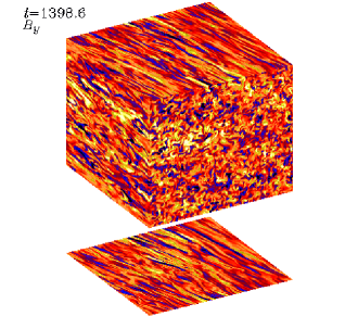
Figure 11: Toroidal magnetic field component displayed on the periphery of the computational domain (color coded). $512^{3}$ meshpoints. $\nu=\eta=2.5\times 10^{-4}\Omega/k_{1}^{2}$.

The simulations presented above may help to determine a critical value of the magnetic Reynolds number, $R_{\rm m}^{\rm(crit)}$, above which dynamo-generated turbulence becomes possible. If the turbulence in the simulation with $256^{3}$ meshpoints remains indeed sustained, we expect $R_{\rm m}^{\rm(crit)}$ to be between 100 and 200. However, the values of $\alpha_{\rm SS}$ are not converged in any of the simulations in that its value increases with resolution, and it is also much larger in the simulations with hyperviscosity than with ordinary viscosity.

5 Spherical Couette flow (preliminary)

In order to better understand the experimental verification of the MRI in spherical Taylor-Couette flow by the Maryland group Sisan et al. (2004), it is desirable to perform simulations that are related to the setup used in the laboratory. We know already that cylindrical Taylor-Couette flow can well be modeled by embedding the flow in a cartesian box Dobler et al. (2002). We also know that simulations of the geodynamo (convection-driven dynamos in a spherical shell) can successfully be modeled by embedding the spherical shell in a box McMillan and Sarson (2003). It is therefore natural to attempt modeling of the Maryland MRI experiment using the same setup. In Fig. 12 we present some preliminary results of spherical Couette flow embedded in a cartesian box with an imposed axial magnetic field of given strength. We work in SI units and chose parameters that are closely related to the experimental setup. A sphere of radius $R=0.15\,{\rm m}$ is embedded in a box of size $(2\times 0.18\,{\rm m})^{3}$. The sphere spins with an angular frequency of $\Omega=300\,{\rm s}^{-1}$. Outside the sphere the velocity is damped to zero at rate $\tau_{\rm damp}^{-1}=200\,{\rm s}^{-1}$. The density is initially uniform and equal to $\rho=930\,{\rm kg}\,{\rm m}^{-3}$. For reasons of computational simplicity our simulation is weakly compressible, and we use an isothermal equation of state (ratio of specific heats is $\gamma=1$) with sound speed $c_{\rm s}=50\,{\rm m}\,{\rm s}^{-1}$. For the present simulations no attempt is made to use realistic values of the kinematic viscosity and the magnetic diffusivity; both are chosen equally big with $\nu=\eta=2\times 10^{-3}\,{\rm m}^{2}\,{\rm s}^{-1}$. The field strength is varied between $500\,{\rm G}$ and $2\,{\rm kG}$.

It turns out that for weak and strong fields the magnetic field is completely axisymmetric. For an intermediate field strength of $B_{0}=1\,{\rm kG}$ both the flow and the magnetic field become nonaxisymmetric.

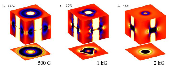
Figure 12: Images of the vertical component of the magnetic field, $B_{z}$, for three different values of the imposed field, $B_{0}$. The images shown on the two side walls of the box go actually through the axis ($x=y=0$), the top plane goes through $z=0.09\,{\rm m}$ and the bottom plane goes through $z=0$.

As anticipated by R. Hollerbach (private communication), the main reason this simulation produces nonaxisymmetric flows is the modification of the background flow in such a way that it becomes Rayleigh unstable, i.e. $q\equiv-{\rm d}{}\ln\Omega/{\rm d}{}\ln r>2$. On the other hand, this does not seem to be the case in the Maryland experiment where the flow remains close to keplerian, i.e. $q\approx 1.5$.

6 Conclusions

The main outcome of the magnetorotational instability is by now well known and its importance for astrophysical discs is obvious. Many details, however, remain far from clear due to the fact that many of the numerical shearing sheet simulations invoke artificial viscosity which is hard to quantify. Thus, we have no clear idea about the critical value of the magnetic Reynolds number required for the combined magnetorotational and dynamo instabilities. The present work suggests that the number is around 200, and certainly above 100, but obviously a more quantitative study would be desirable. Furthermore, details of the nonlinear mode interactions are not well understood. This would be very useful for obtaining a clearer picture of how in the shearing sheet approximation the nonaxisymmetric MRI leads to sustained growth. The Pencil Code is well suited for such studies, and it is publicly available, so it may be hoped that the remaining gaps in our understanding will soon be filled by new members of the scientific community.

Regarding spherical Couette flow, the present approach using embedded box simulations may not be optimal, and dedicated codes for spherical geometry may be advantageous. However, any independent verification using different methods is still often useful. Returning to the astrophysical context, it is important to assess the relative importance of dynamo-generated fields relative to those generated on a more global scale in the rest of the disc. This question can only be appropriately in a fully global simulation. Indeed, significant progress has recently been made in this direction Hawley (2000, 2001); Hawley and Krolik (2001); De Villiers and Hawley (2003).

References

- Balbus and Hawley (1998) Balbus, S. A., and Hawley, J. F., Rev. Mod. Phys, 70, 1–53 (1998).
- Balbus et al. (1996) Balbus, S. A., Hawley, J. F., and Stone, J., Astrophys. J., 467, 76–86 (1996).
- Balbus and Hawley (1991) Balbus, S. A., and Hawley, J. F., Astrophys. J., 376, 214–222 (1991).
- Ogilvie and Pringle (1996) Ogilvie, G. I., and Pringle, J. E., Monthly Notices Roy. Astron. Soc., 279, 152–164 (1996).
- Goldreich and Lynden-Bell (1965) Goldreich, P., and Lynden-Bell, D., Monthly Notices Roy. Astron. Soc., 130, 125–158 (1965).
- Balbus and Hawley (1992a) Balbus, S. A., and Hawley, J. F., Astrophys. J., 400, 610–621 (1992a).
- Foglizzo and Tagger (1994) Foglizzo, T., and Tagger, M., Astron. Astrophys., 287, 297–319 (1994).
- Foglizzo and Tagger (1995) Foglizzo, T., and Tagger, M., Astron. Astrophys., 301, 293–308 (1995).
- Brandenburg and Dintrans (2001) Brandenburg, A., and Dintrans, B., Transient growth in a shearing stratified atmosphere, Tech. rep., NORDITA (2001), URL astro-ph/0111313.
- Kim and Ostriker (2000) Kim, W.-T., and Ostriker, E. C., Astrophys. J., 540, 372–403 (2000).
- Balbus and Hawley (1992b) Balbus, S. A., and Hawley, J. F., Astrophys. J., 392, 662–666 (1992b).
- Brandenburg et al. (1995) Brandenburg, A., Nordlund, A., Stein, R. F., and Torkelsson, U., Astrophys. J., 446, 741–754 (1995).
- Hawley et al. (1995) Hawley, J. F., Gammie, C. F., and Balbus, S. A., Astrophys. J., 440, 742–763 (1995).
- Matsumoto and Tajima (1995) Matsumoto, R., and Tajima, T., Astrophys. J., 445, 767–779 (1995).
- Begelman et al. (1984) Begelman, M. C., Blandford, R. D., and Rees, M. J., Rev. Mod. Phys, 56, 255–351 (1984).
- Frank et al. (1992) Frank, J., King, A. R., and Raine, D. J., Accretion power in astrophysics, Cambridge University Press, 1992.
- Campbell (1997) Campbell, C. G., Magnetohydrodynamics in Binary Stars, Kluwer Academic Publishers, Dordrecht, 1997.
- Shakura and Sunyaev (1973) Shakura, N. I., and Sunyaev, R. A., Astron. Astrophys., 24, 337–355 (1973).
- Brandenburg et al. (1996) Brandenburg, A., Nordlund, A., Stein, R. F., and Torkelsson, U., Astrophys. J. Lett., 458, L45–L48 (1996).
- Brandenburg (1998) Brandenburg, A., “Disc Turbulence and Viscosity,” in Theory of Black Hole Accretion Discs, edited by M. A. Abramowicz et al., Cambridge University Press, 1998, pp. 61–86.
- Hawley et al. (1996) Hawley, J. F., Gammie, C. F., and Balbus, S. A., Astrophys. J., 464, 690–703 (1996).
- Stone et al. (1996) Stone, J. M., Hawley, J. F., Gammie, C. F., and Balbus, S. A., Astrophys. J., 463, 656–673 (1996).
- Miller and Stone (2000) Miller, K. A., and Stone, J. M., Astrophys. J., 534, 398–419 (2000).
- Brandenburg (2001) Brandenburg, A., Astrophys. J., 550, 824–840 (2001).
- Ziegler and Rüdiger (2000) Ziegler, U., and Rüdiger, G., Astron. Astrophys., 356, 1141–1148 (2000).
- Haugen and Brandenburg (2004) Haugen, N. E. L., and Brandenburg, A., Phys. Rev., E70, 1–7 (2004).
- Brandenburg and Sarson (2002) Brandenburg, A., and Sarson, G. R., Phys. Rev. Lett., 88, 1–4 (2002).
- Sisan et al. (2004) Sisan, D. R., Mujica, N., Tillotson, W. A., Huang, Y.-M., Dorland, W., Hassam, A. B., Antonsen, T. M., and Lathrop, D. P., Phys. Rev. Lett., 93, 114502 (2004).
- Dobler et al. (2002) Dobler, W., Shukurov, A., and Brandenburg, A., Phys. Rev., E65, 1–13 (2002).
- McMillan and Sarson (2003) McMillan, D. G., and Sarson, G. R., Am. Geophys. Union, GPC11C, 0280 (2003).
- Hawley (2000) Hawley, J. F., Astrophys. J., 528, 462–479 (2000).
- Hawley (2001) Hawley, J. F., Astrophys. J., 554, 534–547 (2001).
- Hawley and Krolik (2001) Hawley, J. F., and Krolik, J. H., Astrophys. J., 548, 348–367 (2001).
- De Villiers and Hawley (2003) De Villiers, J.-P., and Hawley, J. F., Astrophys. J., 592, 1060–1077 (2003).