Simulating Astro-E2 Observations of Galaxy Clusters: the Case of Turbulent Cores Affected by Tsunamis

Abstract

This is the first attempt to construct detailed X-ray spectra of clusters of galaxies from the results of high-resolution hydrodynamic simulations and simulate X-ray observations in order to study velocity fields of the intracluster medium (ICM). The hydrodynamic simulations are based on the recently proposed tsunami model, in which cluster cores are affected by bulk motions of the ICM and turbulence is produced. We note that most other solutions of the cooling flow problem also involve the generation of turbulence in cluster cores. From the mock X-ray observations with Astro-E2 XRS, we find that turbulent motion of the ICM in cluster cores could be detected with the satellite. The Doppler shifts of the metal lines could be used to discriminate among turbulence models. The gas velocities measured through the mock observations are consistent with the line-emission weighted values inferred directly from hydrodynamic simulations.

1 Introduction

The advent of Astro-E2 (Inoue, 2003) will enable us to directly measure velocity fields of the intracluster medium (ICM) in clusters of galaxies for the first time. The calorimeter (X-Ray Spectrometer; XRS) of Astro-E2 has an excellent spectroscopic resolving power (Kelley, 2004; Cottam et al., 2004), and it could detect the bulk gas motion by observing the energy shift of metal lines and the turbulence by observing broadened metal lines. On the other hand, many hydrodynamic simulations have been performed to study the motion of the ICM (e.g. Evrard, 1990; Takizawa, 1999; Yoshikawa et al., 2000; Ricker & Sarazin, 2001). With Astro-E2, we could confirm the results of those hydrodynamic simulations. However, the direct comparison of X-ray observations to hydrodynamic simulations is not always simple, because of complex such as instrumental responses.

In this paper, we construct the X-ray spectra from the results of hydrodynamic simulations of cluster cores affected by ‘tsunamis’ (Fujita, Matsumoto, & Wada, 2004, hereafter Paper I, see also Fujita, Suzuki, & Wada 2004) and we simulate observations with Astro-E2 XRS. In the tsunami model, large-scale bulk gas motions in the ICM, which are called tsunamis, induce fully-developed turbulence in cluster cores. The ultimate spectroscopic capability of XRS with an energy resolution of $\sim 6$ eV at 6 keV for extended sources as well as point sources could give us a new approach to detect the turbulence in the ICM. Because of the kinetic energy of turbulence and the hot gas brought into the core by turbulent mixing, the radiative heating of the core is suppressed. Thus, this model could solve the so-called ‘cooling flow problem’ (Makishima et al., 2001; Peterson et al., 2001; Kaastra et al., 2001; Tamura et al., 2001).

From the mock observations with Astro-E2, we measure velocity fields of the ICM and compare them with the emission weighted values inferred directly from the hydrodynamic simulations. We investigate whether the former is consistent with the latter. Most observations of clusters scheduled as Astro-E2 performance verification targets in the first 6 months are planned pointing at their centers; one of the reasons is that the effective area of the XRS is relatively small and objects must be bright enough to be observed. Thus, it would be useful to simulate the observations focused on cluster cores. It should be noted that other solutions of the cooling flow problem besides the tsunamis, especially those based on AGN activities, also predict similar level of turbulence in cluster cores, which some observations have already suggested (e.g, Blanton et al., 2001; Churazov et al., 2002; Brüggen & Kaiser, 2002; Kim & Narayan, 2003; Kaiser & Binney, 2003; Fabian et al., 2003; Soker et al., 2004). In this paper, we assume that $\Omega_{0}=0.27$, $\lambda=0.73$, and $H_{0}=70\rm\;km\;s^{-1}\;Mpc^{-1}$.

2 Construction of X-Ray Spectra

We use the results of hydrodynamic simulations done in Paper I. These simulations are performed using a two-dimensional (cylindrically symmetric) nested grid code (Matsumoto & Hanawa, 2003), and the coordinates are represented by $(R,z)$. Since the structure of turbulence in the axi-symmetric coordinate might be different from that in the fully three-dimensional coordinate, it is ideal to perform three-dimensional calculations. However, a high spatial resolution with a large dynamic range is also crucial to simulate a turbulent medium, especially for the tsunami model. Therefore we here restrict the calculations to two dimensions. The cluster center corresponds to $(R,z)=(0,0)$. Although the maximum resolution of the simulations is achieved on the level of grids of 22 pc, we use the simulation results on the level of the grids of 1.4 kpc, because the turbulent velocity is generally smaller on smaller scales and it helps us reduce the number of computational grid points for which we calculate the spectra. We will argue that the effect of the lower resolution on the X-ray spectra can be ignored in §4. Note that in the nested grid code we used, calculations are performed on all grid levels simultaneously. At the cluster center, for example, the solutions (density, temperature, etc.) are obtained on the seven different resolutions. The results of the lower resolution grids are just the coarsened ones of the higher resolution grids.

We use the simulation results for $256\times 512$ computational grid points. For each grid point, we calculate the X-ray spectrum using a single bapec thermal model and the data simulation command fakeit in the XSPEC package (version 11.3.1). The bapec model is the same as the apec model but includes a parameter for turbulent velocity broadening to emission lines. The input parameters of the spectrum for the $i$-th grid point are the temperature ($T_{i}$), the metal abundance ($Z_{i}$), the gas velocity along the line of sight ($v_{i}$), and the normalization. The turbulent velocity for each grid point is assumed to be zero, that is, the gas velocity is uniform within a single grid point. We used the Astro-E2 XRS response file (xrs_ao1.rmf) and the auxiliary file (xrs_onaxis_open_ao1.arf) provided by the Astro-E2 team as planning tools for AO-1 proposals. Weighting the three-dimensional volumes of the grid points, the spectra are summed up by the FTOOLS manipulation task mathpha. In order to avoid the error caused by small photon counts, we multiply the photon counts for each grid point by 100000. After the summation by mathpha, the total photon counts are divided by 100000 using the fcalc task in the FTOOLS. Since fcalc discard fractions in the calculation of the photon counts, we add 50000 to the counts before the division in order to round off. For the resultant spectrum, the error of photon counts in each energy bin is assumed to be the square root of the photon counts in the bin. Background emission and Galactic absorption are ignored. We do not consider the effect of resonance scattering for metal emission lines, because the calculation of multi-dimensional radiative transfer is required and it is beyond the scope of this paper.

3 Results

In paper I, we calculated the evolution of the cool core of a cluster for $R\lesssim 300$ kpc and $|z|\lesssim 300$ kpc. We approximated the bulk gas motions in a cluster by plane wave-like velocity perturbations in the $z$-direction represented by $\delta v_{z}=\alpha c_{s}\sin(2\pi c_{s}t/\lambda)$ at $z=-345$ kpc, where $c_{s}$ is the initial sound velocity, and $\lambda$ is the wave length. The waves propagate in the $z$-direction. At $t=0$, the cluster is isothermal ($T=7$ keV). Metal abundance is uniform and $Z=0.3\>Z_{\sun}$. We construct X-ray spectra for two models with different $\lambda$ (Table 1). The model of $\alpha=0.3$ and $\lambda=100$ kpc (Model A) was studied in Paper I. The model of $\alpha=0.3$ and $\lambda=1000$ kpc (Model B) is newly studied and the detailed analysis of the results will be discussed elsewhere (Matsumoto, Fujita, & Wada 2004, in preparation). Compared to Model A, Rayleigh-Taylor and Kelvin-Helmholtz instabilities develop on larger scales in Model B. This makes turbulent mixing and heating more effective.

We assume that the model cluster is at redshifts of 0.01, 0.04, and 0.08, although the temperature outside of the core is $\sim 7$ keV and there is no such a high-temperature cluster at redshift of 0.01. Since the field of view of Astro-E2 XRS is $2.9^{\prime}\times 2.9^{\prime}$, we consider the X-ray emission within a radius of $1.5^{\prime}$ from the cluster center. At redshifts of 0.01, 0.04, and 0.08, the angle of $1.5^{\prime}$ corresponds to 18.5, 71.3, and 136 kpc, respectively. We ‘observe’ the model cluster along the $z$-axis, that is, the line of sight is assumed to be parallel to the $z$-axis. This is because the waves were injected along that axis, and thus the ICM velocity in the $z$-direction is much larger than that in the $R$-direction. Thus, we sum up the spectra of the ICM in individual grid points for $R<18.5$, 71.3, and 136 kpc and $|z|<300$ kpc for the cluster at redshifts of 0.01, 0.04, and 0.08, respectively. This means that for a cluster at a larger redshift, we observe a larger area. The assumed exposure time is 50 ks. Using XSPEC, we fit the summed spectra with a single bapec model. The spectra were grouped to have a minimum of 50 counts per bin. We limited the energy range to 5–10 keV (at the cluster-rest frames) that includes Fe–K lines ($\sim 6.7$ keV). Free parameters in the bapec model are the temperature ($T$), the metal abundance ($Z$), the average velocity ($v_{z,sp}$), the turbulent velocity ($\sigma_{z,sp}$), and the normalization. We choose $t=3.3$ Gyr for Model A; the temperature distribution at that time is shown in Paper I. We choose $t=5.0$ Gyr for Model B. For Model A, the gas temperature in at least one of the grid points reaches zero at $t=3.3$ Gyr (Paper I), while for Model B, it reaches zero at $t=6.2$ Gyr. Note that the time-scale of 6.2 Gyr is comparable to the typical age of clusters (e.g. Kitayama & Suto, 1996), and thus radiative cooling is almost completely suppressed in Model B.

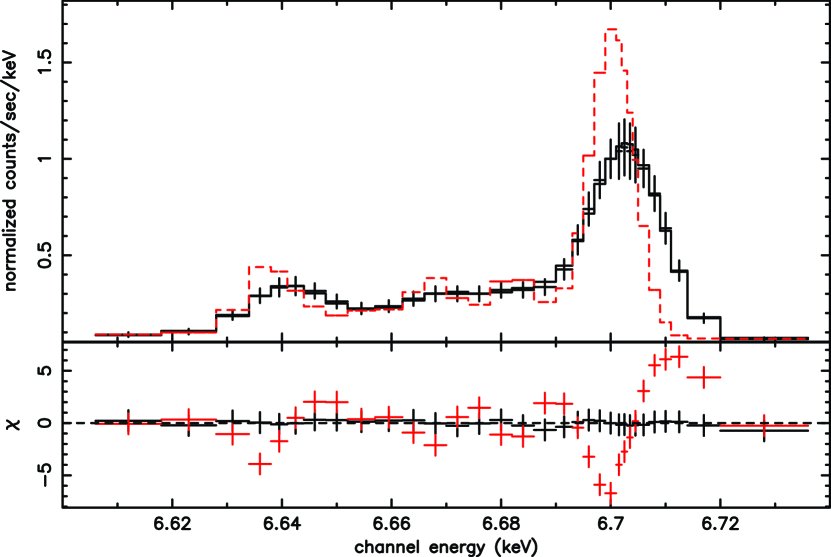
Figure 1: Upper panel shows the simulated X-ray spectrum observed with Astro-E2 XRS for Model B at redshift of 0.04 (crosses) and the best-fit model (solid line). The spectrum when $v_{z,sp}=0$ and $\sigma_{v,sp}=0$ is also shown (dashed line). The spectra are shown at the cluster-rest frame. The lower panel plots the residuals divided by the $1\sigma$ errors.

Figure 1 shows the simulated X-ray spectrum around $6.7$ keV Fe–K lines for Model B at redshift of 0.04 and the result of the fit. For comparison, the spectrum when $v_{z,sp}=0$ and $\sigma_{z,sp}=0$ is also shown. As can be seen, the two spectra (i.e. with and without turbulent motion) are remarkably different. The results of the spectral fits for all models are shown in Table 2. Errors on fitted spectral parameters are given at the 90% confidence level. In Figure 2, we show $v_{z,sp}$ and $\sigma_{z,sp}$. Most models require non-zero turbulent velocity. The values of $\chi^{2}$ are generally small and the fits are good. The results show that the line shift and turbulence will be detected with Astro-E2 XRS if $v_{z,sp}\gtrsim 100\>\rm km\>s^{-1}$ and $\sigma_{z,sp}\gtrsim 100\>\rm km\>s^{-1}$, because $v_{z,sp}=0$ and $\sigma_{z,sp}=0$ are rejected, respectively (Table 2). However, it should be noted that our results correspond to an ideal case. For example, we did not consider possible systematic errors remaining even after calibrations. Moreover, if the line of sight is perpendicular to the $z$-axis, observed average and turbulent velocities are smaller. Thus, turbulence could not be detected for all clusters.

For comparison, we present the luminosity-weighted turbulent velocities in the $z$-direction that are directly derived from the results of hydrodynamic simulations. They are given by

$$\sigma_{z,l}\equiv\sqrt{\frac{\sum_{i}(v_{z,i}-v_{z,l})^{2}L_{i}}{\sum_{i}L_{i}}}\;,$$ (1)

where $v_{z,i}$ is the gas velocity in the $z$-direction, and $L_{i}$ is the luminosity of the $i$-th grid point. As for the luminosity, we consider both the bolometric luminosity, $L_{bol,i}$, and the Fe–K-line luminosity $L_{Fe,i}$. Using XSPEC and the bapec model, we found that the emissivity to be used for the latter is approximately given by

$$\epsilon_{Fe} = 5.559\times 10^{-24}n_{e}n_{\rm H}Z\>\>{\rm ergs\>cm^{-3}s^{-1}}$$

$$\times\left[\frac{25.48\>(0.2917+T)^{2}}{13.14+(0.00169+T)^{2}}+1-4.215\>T+0.2492\>T^{2}-0.005255\>T^{3}\right]\>,$$

for the 6.6–6.72 keV band, where $T$ is the ICM temperature (keV), $Z$ is the metal abundance ($Z_{\sun}$), and $n_{e}$ and $n_{\rm H}$ are the electron density and the hydrogen density ($\rm cm^{-3}$), respectively. This approximation holds within a few percent for $1.5\leq T\leq 15$ keV (even at $T\sim 1$ keV, the error is $\lesssim 10$ %). We ignore the Fe–K emission from the ICM of $T<1.5$ keV, because $\epsilon_{Fe}\approx 0$ and the mass of such gas is small in our calculations. In equation (1), the average gas velocity in the $z$-direction, $v_{z,l}$, is given by

$$v_{z,l}\equiv\frac{\sum_{i}v_{z,i}L_{i}}{\sum_{i}L_{i}}\;.$$ (3)

We refer to $\sigma_{z,l}$ and $v_{z,l}$ weighted by the bolometric luminosities as $\sigma_{z,l,bol}$ and $v_{z,l,bol}$, respectively, and those weighted by the Fe–K luminosities as $\sigma_{z,l,{\rm Fe}}$ and $v_{z,l,{\rm Fe}}$, respectively. The velocities are shown in Figure 2 and $\sigma_{z,l,{\rm Fe}}$ and $v_{z,l,{\rm Fe}}$ are also shown in Table 2.

4 Discussion

In Figure 1, the line profiles appear nearly symmetric. This is because the probability distribution function for $v_{z}$ is almost symmetric (Matsumoto et al. 2004, in preparation). Recently, Inogamov & Sunyaev (2003) investigated line emission from turbulent gas in detail and indicated that line profiles could be very complicated; asymmetry would be observed in the X-ray spectra. However, for the turbulence we considered, the expected asymmetry is too small to be detected with the energy resolution of Astro-E2 XRS. On the other hand, the asymmetric injection of tsunamis is observed as a large offset of $v_{z}\sim-140\>\rm km\>s^{-1}$ (Model B; Table 2), because the asymmetric tsunamis (e.g. those created by cluster mergers) sometimes induce not only the turbulence but also the bulk motion (or oscillation) of the cool core; the latter is unlikely to be induced by symmetric jets accompanied by AGN activities. Therefore, the relative motion between the cD galaxy (stars) and the strongly turbulent core (gas) in a cluster could be a clue to confirm the tsunami model as well as the detection of turbulence in clusters without AGN activities.

Figure 2 shows that $v_{z,sp}$ and $v_{z,l,{\rm Fe}}$ are consistent, and also show that $\sigma_{z,sp}$ and $\sigma_{z,l,{\rm Fe}}$ are consistent. These mean that velocity fields obtained through hydrodynamic simulations can directly be compared with X-ray observations without resorting to mock observations like the one we did here, if the velocities are weighted by line-emission. On the other hand, near the cluster center, which means at smaller redshift, in Model A, $v_{z,sp}$ and $\sigma_{z,sp}$ are not consistent with $v_{z,l,bol}$ and $\sigma_{z,l,bol}$, respectively (Figure 2). However, they are consistent in Model B. The difference between Model A and B is because radiative cooling proceeds more and the gas temperature at the cluster center is lower for Model A at $t=3.3$ Gyr than for Model B at $t=5.0$ Gyr. In Model A, the temperature near the cluster center is $<3$ keV, which is much smaller than the temperature outside of the core ($\sim 7$ keV) and the Fe–K emission is relatively weak. Since cooler gas tends to have larger bulk and turbulent velocities, the gases with larger velocities are less weighted by the Fe–K luminosities. Therefore, in Model A, the velocities weighted by the bolometric luminosities ($|v_{z,l,bol}|$ and $\sigma_{z,l,bol}$) are larger than those weighted by the Fe–K luminosities ($|v_{z,l,{\rm Fe}}|$ and $\sigma_{z,l,{\rm Fe}}$) near the cluster center. On the other hand, in model B, the gas temperature in the central region of the cluster is $\sim 4$ keV and the temperature gradient near the center is small compared to that in Model A. Therefore, $v_{z,l,bol}$ ($\sigma_{z,l,bol}$) and $v_{z,l,{\rm Fe}}$ ($\sigma_{z,l,{\rm Fe}}$) are almost the same.

In Figure 2, the luminosity-weighted turbulent velocities, $\sigma_{z,l,bol}$ and $\sigma_{z,l,{\rm Fe}}$, increase toward the cluster center (toward smaller redshift). This means that the turbulence produced by tsunamis is more detectable at the cluster center.

As mentioned in §2, we used a low resolution grid. However, we expect that the effect of the coarsening on the $v_{z,sp}$ and $\sigma_{z,sp}$ is small, because $v_{z,l,{\rm Fe}}$ and $\sigma_{z,l,{\rm Fe}}$ are not much different in between the low resolution grid and the highest one; the difference is much smaller than the errors of $v_{z,sp}$ and $\sigma_{z,sp}$ presented in Table 2 and Figure 2. Since $v_{z,sp}$ and $v_{z,l,{\rm Fe}}$ ($\sigma_{z,sp}$ and $\sigma_{z,l,{\rm Fe}}$) are almost same as discussed above, $v_{z,sp}$ ($\sigma_{z,sp}$) will not change much even for the finest grid.

We also ‘observed’ the cluster from the direction perpendicular to the $z$-axis and we call this direction $x$. Because of the symmetry we assumed, the average velocities, $v_{x}$, are zero. The turbulent velocities derived from the mock observations are $\sigma_{x,sp}\approx 60$ and $120~{}\rm\>km\>s^{-1}$ for Model A and B, respectively. Consistency between $\sigma_{x,sp}$ and those weighted by Fe–K lines, $\sigma_{x,l,Fe}$, is also good.

5 Conclusions

We have constructed X-ray spectra from the results of hydrodynamic simulations of clusters of galaxies based on the tsunami model, in which turbulence is created in cluster cores. Similar levels of turbulence are also predicted by many of other heating models of cool cores (e.g. motion of bubbles created by AGN activities; Churazov et al., 2002; Brüggen & Kaiser, 2002). In particular, we focus on the effect of velocity fields of the ICM on the spectra. We simulate X-ray observations with Astro-E2 XRS and find that velocity fields in cluster cores could be revealed with the satellite. The motion of the cool core could be used to discriminate among turbulence models We show that the gas velocities derived through the mock observations are consistent with the Fe–K line emission weighted values inferred directly from hydrodynamic simulations. The technique developed here could easily be applied to the comparison between results of various hydrodynamic simulations and those of near-future observations with Astro-E2 and others (Constellation-X, XEUS, NeXT).

Table 1: Model Parameters

Model	$\alpha$	$\lambda$ (kpc)	$t$ (Gyr)
A	0.3	100	3.3
B	0.3	1000	5.0

Table 2: Fitting Results

Model	$T$	$Z$	$v_{z,sp}$	$\sigma_{z,sp}$	$\chi^{2}/$dof	$v_{z,l,{\rm Fe}}$	$\sigma_{z,l,{\rm Fe}}$	$F_{x}$ (5–10 keV)
(Redshift)	(keV)	($Z_{\sun}$)	($\rm km\>s^{-1}$)	($\rm km\>s^{-1}$)		($\rm km\>s^{-1}$)	($\rm km\>s^{-1}$)	($\>\rm erg\>cm^{-2}\>s^{-1}$)
A (0.01)	$2.80_{-0.05}^{+0.06}$	$0.26_{-0.01}^{+0.01}$	$10_{-5}^{+15}$	$123_{-12}^{+14}$	217.6/679	12	124	$1.1\times 10^{-10}$
A (0.04)	$4.55_{-0.19}^{+0.20}$	$0.28_{-0.02}^{+0.02}$	$-2_{-16}^{+13}$	$81_{-34}^{+26}$	122.8/241	-2	83	$3.2\times 10^{-11}$
A (0.08)	$5.71_{-0.47}^{+0.41}$	$0.30_{-0.03}^{+0.03}$	$5_{-28}^{+25}$	$82_{-82}^{+54}$	170.4/95	2	80	$1.2\times 10^{-11}$
B (0.01)	$4.04_{-0.09}^{+0.11}$	$0.29_{-0.01}^{+0.01}$	$-147_{-10}^{+21}$	$256_{-11}^{+13}$	163.8/724	-150	237	$1.1\times 10^{-10}$
B (0.04)	$4.44_{-0.19}^{+0.17}$	$0.30_{-0.02}^{+0.02}$	$-123_{-21}^{+22}$	$230_{-21}^{+22}$	128.5/283	-128	214	$3.8\times 10^{-11}$
B (0.08)	$4.81_{-0.33}^{+0.36}$	$0.29_{-0.03}^{+0.03}$	$-153_{-36}^{+33}$	$203_{-39}^{+39}$	88.2/104	-158	201	$1.4\times 10^{-11}$

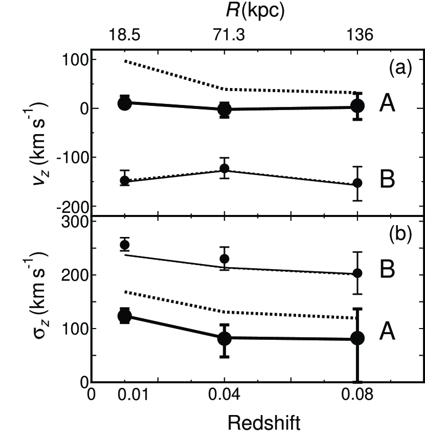
Figure 2: (a) Average gas velocities for different redshifts. Radii corresponding to the field of view of XRS ($R$) are also shown. Dotted lines indicate$v_{z,l,bol}$ andsolid lines indicate $v_{z,l,{\rm Fe}}$. Filled circles indicate $v_{z,sp}$. Bold lines and large circles correspond to Model A and thin lines and small circles correspond to Model B. (b) Turbulent velocities for different redshifts. Dotted lines indicate $\sigma_{z,l,bol}$ and solid lines indicate $\sigma_{z,l,{\rm Fe}}$. Filled circles indicate $\sigma_{z,sp}$. Bold lines and large circles correspond to Model A and thin lines and small circles correspond to Model B.

References

- Blanton et al. (2001) Blanton, E. L., Sarazin, C. L., McNamara, B. R., & Wise, M. W. 2001, ApJ, 558, L15
- Brüggen & Kaiser (2002) Brüggen, M., & Kaiser, C. R. 2002, Nature, 418, 301
- Churazov et al. (2002) Churazov, E., Sunyaev, R., Forman, W., & Böhringer, H. 2002, MNRAS, 332, 729
- Cottam et al. (2004) Cottam, J., et al. 2004, Nuclear Instruments and Methods in Physics Research A, 520, 368
- Evrard (1990) Evrard, A. E. 1990, ApJ, 363, 349
- Fabian (1994) Fabian, A. C. 1994, ARA&A, 32, 277
- Fabian et al. (2003) Fabian, A. C., Sanders, J. S., Allen, S. W., Crawford, C. S., Iwasawa, K., Johnstone, R. M., Schmidt, R. W., & Taylor, G. B. 2003, MNRAS, 344, L43
- Fujita et al. (2004) Fujita, Y., Matsumoto, T., & Wada, K. 2004, ApJ, 612, L9
- Fujita, Suzuki, & Wada (2004) Fujita, Y., Suzuki, T. K., & Wada, K. 2004, ApJ, 600, 650
- Inogamov & Sunyaev (2003) Inogamov, N. A., & Sunyaev, R. A. 2003, Astronomy Letters, 29, 791
- Inoue (2003) Inoue, H. 2003, SPIE, 4851, 289 (http://astroe2.gsfc.nasa.gov/docs/astroe/prop_tools/astroe2_td/)
- Kaastra et al. (2001) Kaastra, J. S., Ferrigno, C., Tamura, T., Paerels, F. B. S., Peterson, J. R., & Mittaz, J. P. D. 2001, A&A, 365, L99
- Kaiser & Binney (2003) Kaiser, C. R. & Binney, J. 2003, MNRAS, 338, 837
- Kelley (2004) Kelley, R. L. 2004, Nuclear Instruments and Methods in Physics Research A, 520, 364
- Kim & Narayan (2003) Kim, W., & Narayan, R. 2003, ApJ, 596, L139
- Kitayama & Suto (1996) Kitayama, T., & Suto, Y. 1996, ApJ, 469, 480
- Makishima et al. (2001) Makishima, K., et al. 2001, PASJ, 53, 401
- Matsumoto & Hanawa (2003) Matsumoto, T., & Hanawa, T. 2003, ApJ, 595, 913
- Peterson et al. (2001) Peterson, J. R., et al. 2001, A&A, 365, L104
- Ricker & Sarazin (2001) Ricker, P. M., & Sarazin, C. L. 2001, ApJ, 561, 621
- Soker et al. (2004) Soker, N., Blanton, E. L., & Sarazin, C. L. 2004, A&A, 422, 445
- Takizawa (1999) Takizawa, M. 1999, ApJ, 520, 514
- Tamura et al. (2001) Tamura, T., et al. 2001, A&A, 365, L87
- Yoshikawa et al. (2000) Yoshikawa, K., Jing, Y. P., & Suto, Y. 2000, ApJ, 535, 593