Depth Development of Extensive Air Showers from Muon Time Distributions

Abstract

We develop an algorithm that has the potential to relate the depth development of ultra high energy extensive air showers and the time delay for individual muons. The time distributions sampled at different positions at ground level by a large air shower array are converted into distributions of production distances using an approximate relation between production distance, transverse distance and time delay. The method is naturally restricted to inclined showers where muons dominate the signal at ground level but could be extended to vertical showers provided that the detectors used can separate the muon signal from electrons and photons. We explore the accuracy and practical uncertainties involved in the proposed method. For practical purposes only the muons that fall outside the central region of the shower can be used, and we establish cuts in transverse distance. The method is tested using simulated showers by comparing the production distance distributions obtained using the method with the actual distances in the simulated showers. It could be applied in the search for neutrinos to increase the acceptance to highly penetrating particles, as well as for unraveling the relative compositions of protons and heavy nuclei. We also illustrate that the obtained depth distributions have minimum width when both the arrival direction and the core position are well reconstructed.

I Introduction

When an Ultra High Energy Cosmic Ray (UHECR) particle enters the atmosphere it interacts producing an extensive air shower that propagates through it and reaches ground level. These showers are routinely detected by optical systems that collect fluorescence light emitted by nitrogen molecules excited as the front crosses the atmosphere, and by arrays of particle detectors that sample at ground level an enormous shower front which can exceed $10^{12}$ particles. In these arrays the relative times of the detected signals allow the reconstruction of the incoming particle arrival direction. The time distribution of the arriving signal has been known for long to be dependent on the depth distribution of the shower particles Lapikens ; Linsley ; Watson ; Antoni:2002vv which is different for different primary particles.

Exploring the highest energy particles is now considered to be a priority because the data are scarce, there are discrepancies between results obtained with the two techniques and because the origin of these particles is not at all understood NaganoWatson . Their study is expected to provide both information on violent objects in the Universe where these particles originate and on their interactions (during propagation and in the atmosphere) at energies exceeding those achieved in accelerator experiments by many orders of magnitude. New experiments are being constructed and devised to improve the statistics, to increase the precision and to establish the mass of the primary particles. The Auger Observatory in Argentina is the first of a new generation of large aperture experiments. It combines the two techniques and for the ground array it uses water Čerenkov tanks with photomultiplier tubes and Flash Analog to Digital Converters (FADC) to record the time stamp of the signal in 25 ns intervals with unprecedented accuracy EA .

The perspective of improved detectors has triggered an increase of phenomenological activity in the study and characterization of extensive air showers. Evaluation of the time structure of showers is part of this effort motivated by both the practical need of controlling the uncertainties in the arrival direction reconstruction and also by the hope that its understanding might shed new light on the challenging problem of establishing their composition. The idea of relating the muon distributions to the shower development has been already quite successful Danilova ; Brancus:1997rr ; Pentchev1 ; Ambrosio:1999nr ; model . The arrival time distributions of muons has been characterized using simple geometrical and kinematical arguments and making a key simplifying assumption on the muon energy, transverse momentum, and distance of production distributions, namely that they are independent cazon3 . Here we have further developed the algorithm that relates the arrival time distribution of muons to the depth development of the shower following on these ideas.

The scope of the method is limited because the shower front contains many other particles, mainly electrons and photons. In principle it requires muon identification but fortunately the muon signal dominates in two circumstances: when the shower is inclined and the electromagnetic part does not reach ground level model but also for “more vertical” showers when the distance to shower axis is sufficiently large rhomu_rsignal . The method complements alternative depth reconstruction methods which are always limited when only densities at ground level are taken into consideration. Moreover when the effects of arrival angle and impact point misreconstruction are taken into account it is seen that the induced distributions have a minimum in their spread for the correct angle and impact point. This effect opens the possibility of using this method for improving the confidence in the conventional angular and impact point reconstructions. While the precision obtained is possibly insufficient to be used for composition studies it will certainly have an important impact on improving the acceptance of air shower arrays to neutrinos through inclined showers. The accuracy in the depth development reconstruction is sufficient to exclude neutrino interactions at intermediate depths, when the electromagnetic shower would have been completely absorbed but the first interaction is sufficiently deep into the atmosphere to exclude both a cosmic ray hadron and a photon.

The article is organized as follows: In Section II we summarize the factorization hypothesis for the muon distributions and the relations that follow, and motivate the inversion of the relation between the time and depth distribution from Ref. cazon3 . We also pay some attention to the relation between particle densities and detector geometric acceptance. In Section III we present the method to reconstruct the depth distribution. In Section IV we compare the depth distributions obtained with this reconstruction method to actual distributions from simulated showers to test it. In Section V discussing some practical limitations. In Section VI we explore the correlations between the reconstruction procedure and the assumed arrival direction and impact point as a check of its robustness; we summarize and conclude in Section VII. Technical details are presented in two appendices.

II Relation between depth development and muon time distributions

The main features of the arrival time distributions of muons in extensive air showers can be accounted for by the different path lengths traveled by the muons from their production point. This has been recently shown using a simplified model to describe the muons in air showers which is based on the hypothesis that their energy, $E_{i}$, transverse momentum, $p_{t}$, production distance, $z$, and outgoing polar angle, $\zeta$ distributions factorize cazon3

$$\frac{d^{4}N_{0}}{dz\;\!d\zeta\;\!dE_{i}\;\!dp_{t}}=\frac{1}{2\pi}{\cal N}_{0}\;\!h(z)\;\!f_{1}(E_{i})\;\!f_{2}(p_{t}),$$ (1)

In this expression $E_{i}$, $p_{t}$ and ${\cal N}_{0}$ refer to production, $z$ is measured along the shower axis from the muon production point to the ground. The transverse momentum is transverse to shower axis and has polar angle $\zeta$ in the transverse plane (perpendicular to shower axis). The functions $h(z)$, $f_{1}(E_{i})$ and $f_{2}(p_{t})$ are assumed independent and normalized to 1 and the factor $2\pi$ accounts for a uniform polar angle distribution. Finally ${\cal N}_{0}$, the total number of produced muons, is the overall normalization. In this model the muons are assumed to travel in straight lines and these four variables are sufficient to determine the muon path uniquely.

It is convenient to express the muon direction in terms of the angle $\alpha$ with respect to shower axis. For a muon produced with energy $E_{i}$ and transverse momentum $p_{t}$, the angle $\alpha$ is given by

$$\sin\alpha=\frac{p_{t}c}{\sqrt{E_{i}^{2}-(mc^{2})^{2}}}\simeq\frac{p_{t}c}{E_{i}},$$ (2)

We can approximate $pc=\sqrt{E_{i}^{2}-(mc^{2})^{2}}\simeq E_{i}$, because the muon energy at ground level is typically greater than $mc^{2}$, this energy at production is even greater because of muon energy loss. We can now change the coordinates replacing $p_{t}$ in Eq. 1 using Eq. 2 to give

$$\frac{d^{4}N_{0}}{dz\;\!d\zeta\;\!dE_{i}\;\!d{\sin{\alpha}}}={\cal N}_{0}\;\!\frac{1}{2\pi}h(z)\;\!f_{1}(E_{i})\;\!f_{2}\left(\frac{E_{i}}{c}\sin{\alpha}\right)\frac{E_{i}}{c}.$$ (3)

As the muons go through the atmosphere they lose energy and decay and even though we start with independent distributions at production, correlations between the relevant variables appear naturally when we consider the surviving muon distribution at ground level. This is explicitly shown in Appendix A using a simplified model for energy loss.

The distribution of surviving muons can then be integrated in $E_{i}$ in order to obtain the depth distribution of the surviving muons, which is given in terms of two angles describing the muon direction, namely $\alpha$ and $\zeta$. It is convenient to relate them to the differential solid angle for the muon $d^{2}\Omega=-d\zeta d\cos\alpha$. Then

$$\frac{d^{3}N}{dz\;\!d^{2}\Omega}=\frac{d^{3}N}{dz\;\!d\zeta\;\!d\sin{\alpha}}\;\!\frac{\cos{\alpha}}{\sin{\alpha}}.$$ (4)

It is interesting to discuss in some detail the effect of a detector surface. From Eq. 4 we can obtain the number of muons from a given production interval $dz$ that crosses an arbitrary surface $d^{2}A$ which subtends a solid angle $d^{2}\Omega$:

$$dN_{A}=\frac{d^{3}N}{dz\;\!d^{2}\Omega}d^{2}\Omega~{}dz=\frac{d^{3}N}{dz\;\!d^{2}\Omega}\;\!\frac{\cos{\psi_{\mu A}}\;\!d^{2}A}{l^{2}}\;\!dz.$$ (5)

where $\psi_{\mu A}$ is the angle between the normal to the surface and the muon direction. On the other hand the projection of $d^{2}A$ onto the shower transverse plane is $rd\zeta dr=d^{2}A\cos{\psi_{A}}$, where $\psi_{A}$ is the angle between the normal to the surface and the shower direction. (See Fig. 11 in Appendix A.) Using this relation we can relate Eq. 4 to the number of particles per unit area in the transverse plane:

$$\frac{1}{r}\;\!\frac{d^{3}N_{A}}{dz\;\!dr\;\!d\zeta}=\frac{d^{3}N}{dz\;\!d^{2}\Omega}\;\!\frac{1}{l^{2}}\;\!\frac{\cos{\psi_{\mu A}}}{\cos{\psi_{A}}}=\frac{d^{3}N}{dz\;\!d^{2}\Omega}\;\!\frac{1}{l^{2}}D_{A}(\Omega)=\frac{d^{3}N}{dz\;\!d\zeta\;\!d\sin{\alpha}}\;\!\frac{\cos{\alpha}}{\sin{\alpha}}\;\!\frac{1}{l^{2}}D_{A}(\Omega).$$ (6)

Where $D_{A}(\Omega)$ denotes the geometrical factor involving these two angles. We stress that $D_{A}$ not only depends on the surface orientation with respect to shower axis but also on the direction of the incoming muons. Any detector can be regarded as a collection of such surfaces and as a result several such factors $D_{A_{i}}$ will have to be considered depending on the impact point to obtain the total effective collection area for a given arrival direction.

We can divide Eq. 6 by its integral in $z$ ($\hat{N}_{Ar\zeta}$) to normalize the function to 1. When this is done, using plausible functions for the distributions as described in Appendix A, and the relations between $r$, $l$, $z$ and $\alpha$ are used, a number of factors cancel out and we obtain the $z$-distribution of muons arriving at detector $A$ (normalized to 1) which can be related to a simple transform of the $z$ distribution:

$$\frac{1}{{\hat{N}}_{Ar\zeta}}\;\!\frac{1}{r}\;\!\frac{d^{3}N_{A}}{dr\;\!dz\;\!d\zeta}=\frac{h(z)\;\!l^{1-\gamma}\cos\alpha~{}D_{A}(\Omega)}{\int_{0}^{\infty}dz\;\!h(z)\;\!l^{1-\gamma}\cos\alpha~{}D_{A}(\Omega)}.$$ (7)

The proposed method relies on the above expression and the geometrical relation between $z$ and $t$ which is described in Ref. cazon3 . In that work it was shown that much of the time structure of the muons is due to geometrical effects which imply that to each $z$ there corresponds a given arrival time $t$. As a result we can relate the $t$ and $z$-distributions:

$$\frac{1}{r}\;\!\frac{d^{3}N_{A}}{dr\;\!d\zeta\;\!dt}=\frac{1}{r}\;\!\frac{d^{3}N_{A}}{dr\;\!d\zeta\;\!dz}\;\!\frac{dz}{dt}.$$ (8)

We now define the normalized function $g(t)$ describing the shape of the time distribution through:

$${\hat{N}}_{Ar\zeta}\;\!g(t)=\frac{1}{r}\;\!\frac{d^{3}N_{A}}{dr\;\!d\zeta\;\!dz}\Big{|}\;\!\frac{dz}{dt}\Big{|}.$$ (9)

We can compare the $t$-distributions of the muons arriving at ground level given by Eq. 9 to those obtained in simulations and agreement is found as will be shown in Section IV.

The time distribution of the muons is related to the depth distribution of muon production. If we combine Eq. 7 and Eq. 9 we obtain the following relation between $h(z)$ and the time distribution:

$$g(t)\Big{|}\frac{dt}{dz}\Big{|}=\frac{1}{{\hat{N}}_{Ar\zeta}}\;\!\frac{1}{r}\;\!\frac{d^{3}N_{A}}{dr\;\!dz\;\!d\zeta}=\frac{h(z)\;\!l^{1-\gamma}\cos\alpha~{}D_{A}(\Omega)}{\int_{0}^{\infty}dz\;\!h(z)\;\!l^{1-\gamma}\cos\alpha~{}D_{A}(\Omega)}.$$ (10)

This expression takes into account the fact that from different $r$ we effectively sample the $h(z)$ distribution with an extra $z$-dependence introduced as a overall factor through $l$ and the angles $\alpha$ and $\zeta$.

III Reconstruction of the depth distribution

In a typical air shower array a number of particle detectors sample the shower front at the Earth’s surface. We now consider a set of $M$ detectors labeled by a suffix $i$ (from $1$ up to $M$) each with a surface $A_{i}$ (which becomes $S_{i}$ when projected onto the shower plane) and located at position $(r,\zeta)_{i}$ in transverse plane coordinates. We calculate the time distribution of arriving muons to a detector $i$ by integrating Eq. 8 over the transverse surface $dS$, or, for all practical purposes, simply multiplying by the corresponding area $S_{i}$. Using Eq. 9 the time distribution at detector $i$ becomes:

$$\frac{dN_{A}}{dt}\Big{|}_{i}\equiv\int_{S_{i}}\frac{d^{3}N_{A_{i}}}{dt\;\!r\;\!dr\;\!d\zeta}(r,\zeta)dS\simeq S_{i}\hat{N}_{Ar\zeta}~{}g(t).$$ (11)

The number of muons falling in the detector $i$ can be considered as a finite sample of the continuous arrival time distribution probability $\frac{dN_{A}}{dt}\Big{|}_{i}$. Let us assume that we can fill a time histogram with $N_{i}$ entries corresponding to the $N_{i}$ muons detected by detector $i$. The entries of this histogram can be transformed into a $z$ histogram, using the correspondence $t\rightarrow z$ given by cazon3 :

$$z=\frac{1}{2}\left(\frac{r^{2}}{ct}-ct\right)+\Delta,$$ (12)

which can, in most cases, be approximated by:

$$z\simeq\frac{1}{2}\frac{r^{2}}{ct}+\Delta.$$ (13)

This mapping transforms each time entry (from $\frac{dN_{A}}{dt}\Big{|}_{i}\simeq S_{i}\hat{N}_{Ar\zeta}~{}g(t)$ ) into a $z$ entry (of $S_{i}\frac{1}{r}\;\!\frac{d^{3}N_{A}}{dr\;\!d\zeta\;\!dz}$) and finally into an entry of the $z$-distribution of the muons arriving at ground, $\frac{dN}{dz}$.

Note that the delay $t$ is the time difference between the arrival time of a given particle and the arrival time of a reference plane perpendicular to the shower axis and traveling at the speed of light $c$, the time-reference plane. We have chosen the $0$-time origin corresponding to the arrival of the first particle at ground at $r=0$ (shower core). If the core hits ground at a universal time $ct_{0}^{\prime}$, the relation between $t^{\prime}$ and $t$ involves $\Delta$:

$$ct=ct^{\prime}-ct_{0}^{\prime}+\Delta.$$ (14)

Different detectors will give entries to a different time distribution, but they will be converted into samples of a unique $\frac{dN}{dz}$ distribution. As a result the converted entries of available detectors can be combined into a larger sample. These entries are naturally weighted by the number of muons detected at each detector.

In Ref. cazon3 it was shown that there is an additional source of delay for muons because of their sub-luminal velocities $t_{\varepsilon}$. The total time delay is obtained adding it to the delay given by Eq. 13:

$$t\simeq t_{g}+t_{\varepsilon}.$$ (15)

This delay is energy dependent and it is only dominant over the geometric delay for muons close to shower axis. In inclined showers the final muon energy is much larger than the muon mass, $mc^{2}\ll E_{i}-\rho al$, and therefore:

$$t_{\epsilon}\simeq\frac{1}{2}\;\!\frac{(mc^{2})^{2}}{c\rho a}\left[\frac{1}{E_{i}-\rho al}-\frac{1}{E_{i}}\right].$$ (16)

Since the muon energy is not measured in typical air shower measurements, we cannot account for these effects accurately. A solution is simply obtained by eliminating the measurements close to the axis to ensure that the kinematical delay can be neglected. This has an impact on statistics. In Fig. 1 we have plotted the factor $\epsilon(r,z)$, which can be taken as the relative value of the average kinematic delay with respect to the average geometric delay (see Appendix B), for $\zeta=90^{\circ}$, $\Delta=0$ and different $z$. We can see from this graph that the geometric delay dominates for distances above 600 m from shower core.

We can include the kinematic delays on average. We obtain a simple parameterization for the average kinematic delay as a function of $z$ and $r$, (details are given in Appendix B):

$$\epsilon(r,z)=p_{0}(z)\left(\frac{r}{\rm m}\right)^{p_{1}}.$$ (17)

If we now subtract the average kinematical delay from the measured delay, instead of Eq. 12 we obtain:

$$z\simeq\frac{1}{2}\left(\frac{r^{2}}{ct-c<t_{\varepsilon}>}-(ct-c<t_{\varepsilon}>)\right)+\Delta.$$ (18)

Since it is not possible to obtain $z(t)$ analytically from the previous expression we can use a simple numerical approach. We can for instance take zero kinematical delay as a first approximation to obtain $z$, we then get the average kinematical delay and substitute in Eq. 18. Since the dependence of the $p$ coefficients on $z$ is mild (logarithmic) the procedure converges quickly and one iteration is sufficient.

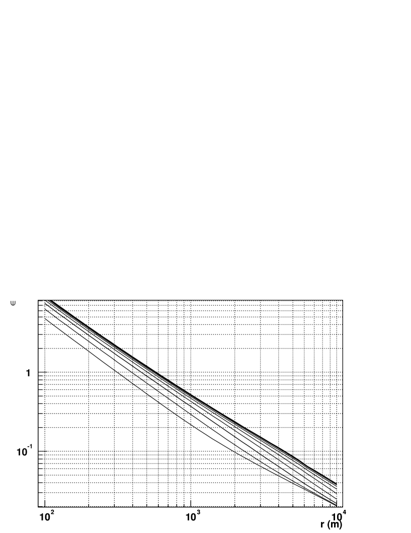
Figure 1: The factor $\epsilon(r,z)$ which relates to the ratio of kinematic to geometric time delays (see text) versus $r$ for different $z$: 1.6, 3.2, 6.3, 13, 25, 50, 100, 200 km, from bottom to top.

IV Test

One approach to test the method is to simulate showers using a Monte Carlo generator that reproduces the time distribution of the signal in a collection of detectors and to apply the method to reconstruct the production distribution of the muons $h(z)$. Unfortunately major modifications have to be made in conventional simulation programs that are not designed to give the function $h(z)$ to compare with the reconstructed value. We have checked our reconstruction method by applying it to showers simulated with the Aires Monte Carlo package Aires . It is straightforward to compare the $z$-distributions of the muons arriving at different locations in the ground. This has been done at different positions and agreement is found. This reflects the fact that the time distributions of the muons are well described by the model for muon time delays cazon3 . We have extended the test to combine detectors at different positions and to compare the results to the total distribution of the surviving muons $dN/dz$, which is straightforward to obtain in Aires and in most shower generators. In our model this distribution would be obtained by integrating Eq. 7 over $r$ and $\zeta$ to cover all the ground:

$$\frac{dN}{dz}=\int\int\;\!\frac{1}{r}\;\!\frac{d^{3}N}{dr\;\!d\zeta\;\!dz}~{}r\;\!dr\;\!d\zeta=\int\int\hat{N}_{r\zeta}\frac{h(z)\;\!l^{1-\gamma}\cos\alpha~{}D_{A}(\alpha)}{\int_{0}^{\infty}h(z)\;\!{l}^{1-\gamma}\cos\alpha~{}D_{A}(\alpha)~{}dz}~{}rdrd\zeta.$$ (19)

Using simulations we have studied how the total $dN/dz$ distribution at ground relates to the local distributions at different $r$, after integrating in $\zeta$ and $r$. We first note that to a first approximation the $\zeta$-integral is proportional to the integrand with $\Delta=0$. This is not surprising since $\Delta$ changes sign when integrating over $\zeta$. We have found that there is an effective value of $r$ ($r_{*}$) for local distribution that gives a very good approximation to the overall $dN/dz$ distribution. This value is slightly zenith angle dependent and ranges from about 400 m for showers at $0^{\circ}$, up to 1000 m for horizontal showers at $80^{\circ}$ or 1800 m at $86^{\circ}$ . This is reasonable because the bulk of the muons arrive to ground in a relatively constrained region: for instance, at $0^{\circ}$ this region is between $\sim 60$ m and $\sim 1000$ m. We can then substitute in Eq. 19 $l$ for $l_{\star}=\sqrt{r_{\star}^{2}+z^{2}}$ and $\alpha$ for $\alpha_{\star}=\arcsin\frac{r_{\star}}{l_{\star}}$ and also consider that to compare with Aires that gives directly the muon position it is not necessary to include a geometric correction factor, i.e. $D_{A}=1$. We finally obtain the following approximation

$$\frac{dN}{dz}\propto h(z)\;\!l_{\star}^{1-\gamma}\cos\alpha_{\star}.$$ (20)

Since in a practical air shower array the detectors are going to be arranged on an unknown and arbitrary pattern around the shower axis it is convenient to correct the $z$-distribution obtained at each detector to a common observation distance $r_{\star}$ which approximately reproduces the overall $dN/dz$ as follows:

$$\frac{dN}{dz}\propto g(t)\Big{|}\frac{dt}{dz}\Big{|}~{}\times~{}\frac{l_{\star}^{1-\gamma}\cos\alpha_{\star}}{l^{1-\gamma}\cos\alpha}\frac{1}{~{}D_{A}(\alpha)}.$$ (21)

In general, we must divide by $D_{A}(\alpha)$ to remove the dependence on the detector geometry if necessary. We note that the correction factors $\frac{l_{\star}^{1-\gamma}\cos\alpha_{\star}}{l^{1-\gamma}\cos\alpha}$ approach 1 when $z$ increases (i.e. in horizontal showers). Taking this into account one can use a single $r_{\star}=400~{}$m for all zenith angles and still obtain relatively good approximations.

To test the method we have used sets of 500 showers at different zenith angles. A given particle array will be limited to a sample of this distribution which is determined by the relative positions of the available detectors. We first take the muon output from the simulations and arrange the muons in a time histogram as can be done in an actual shower array (we use 25 ns bins). We then apply Eq. 18 to all the simulated muons to calculate $z$, where we have included the geometric corrections of Eq. 21 and the kinematic corrections as explained in the previous section. Finally an $r$ cut is applied. In Figs. 2 and 3 we illustrate the result for a $0^{\circ}$ and a $70^{\circ}$ showers. The shaded histogram is the distribution of all the muon production altitudes compared to that obtained from the reconstruction procedure using all the muons which reach the ground with $r>r_{c}$. This cut is necessary for the geometric inversion procedure to hold accurately. The result indicates that provided the muon time, the shower direction and impact point coordinates are known, the reconstruction procedure works well. Figs. 2 and 3 also show the same histogram without the $r$-cut which clearly fails to reproduce the $z$-distribution obtained in the simulation. This is mostly because of the time accuracy of the detectors assumed to be $\sim 12.5~{}$ns.

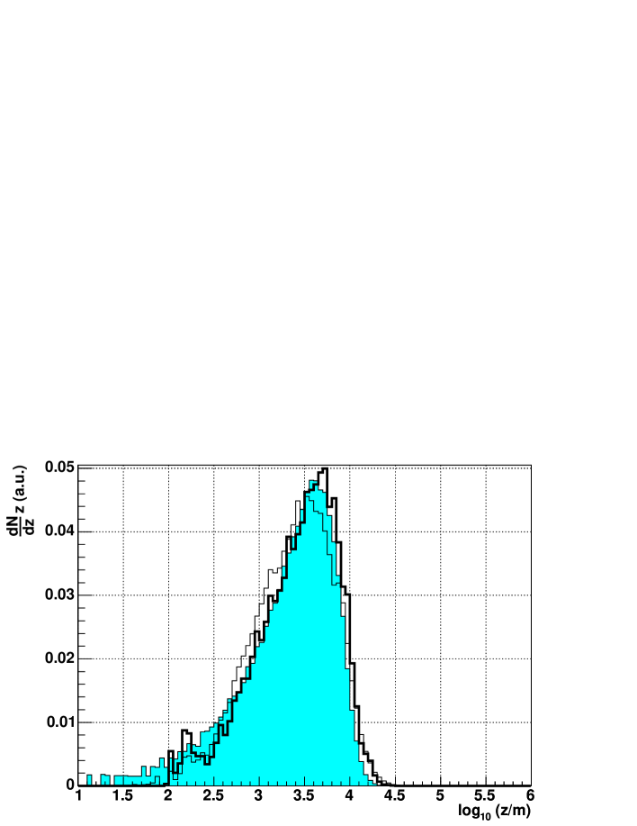
Figure 2: Histograms of production distribution for 500 showers of $0^{\circ}$ zenith angle and $10^{19}$ eV energy: Light fill: original distribution. Unfilled Thick Line: Final reconstruction, after all corrections described in the text. Unfilled Thin Line Reconstruction with no r cut.

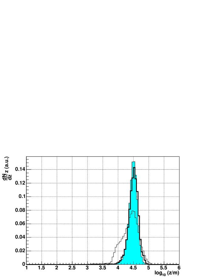
Figure 3: Histograms of production distribution for 500 showers of $70^{\circ}$ zenith angle and $10^{19}$ eV energy: Light fill: original distribution.Unfilled Thick Line: Final reconstruction, after all corrections described in the text. Unfilled Thin Line Reconstruction with no r cut.

We have verified that the reconstructed histogram is not sensitive to small changes in the $r_{c}$ but clearly these cuts in $r$ can have large impact on the statistics. In table 1 we compare the averages of the ratio of $z$ obtained with this method to that from the simulation $\Gamma=<\frac{z_{\rm rec}}{z_{\rm true}}>$. Clearly the method works best for moderately inclined showers between $60^{\circ}$ and $80^{\circ}$. At very low zenith angles, there is an overestimation of the production distance, which could be due to an slight overestimation of the energy loss. On the other hand, at very high zenith angles the magnetic field effects begin to be important and the time geometric relation underestimates the production distance. Nevertheless, in both cases, the precision obtained is quite good.

$\theta\;\;({\rm deg})$	$\phi$ (deg)	B	cut r(m)	$\Gamma$
0	-	no	900	1.23
30	-	no	1000	1.16
60	-	no	1500	1.07
70	-	no	2000	1.03
80	-	no	2900	1.00
80	0	yes	2900	0.97
80	90	yes	2900	0.89
86	0	yes	4000	0.86
86	90	yes	4000	0.85
neutrino-like injected at $500$ ${\rm g/cm^{2}}$ vertical depth.
80	0	yes	1400	1.02
neutrino-like injected at $750$ ${\rm g/cm^{2}}$ vertical depth.
80	0	yes	900	1.14

Table 1: Table of deviation of the reconstruction respect to the real distribution. $\Gamma=<\frac{z_{\rm rec}}{z_{\rm true}}>$. The azimuth angle $\phi$ is measured counterclockwise respect to the local magnetic north. For high zenith angles the results obtained with and without magnetic field are compared.

In Fig. 4 we have compared the results of the reconstruction procedure applied to protons and deeply injected protons arriving with $80^{\circ}$ zenith angle to illustrate how the method can be used to identify deeply interacting inclined showers at high zenith, which are natural neutrino candidates. A systematic study of the reconstruction procedure and the ability to identify neutrinos under realistic experimental conditions is left for future work.

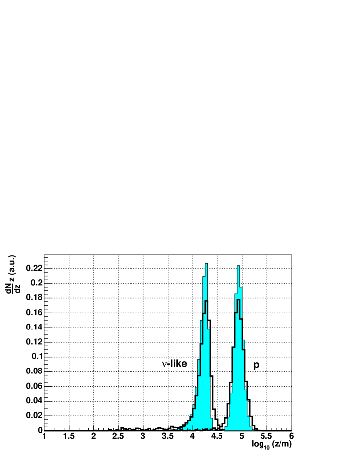
Figure 4: Histograms of production distribution for 500 showers of $80^{\circ}$ zenith angle and $10^{19}$ eV energy for normal protons and for protons injected at 500 ${\rm r/cm^{2}}$ of vertical depth to simulate a neutrino interaction (marked as $\nu$-like). The geomagnetic field is included. Light fill: original distribution. Unfilled Thick Line: Final reconstruction, after all corrections described in the text.

V Limitations of the method

The proposed method gives the reconstruction of the function $\frac{dN}{dz}$ i.e., the production altitude distribution for the surviving muons but clearly the method is only valid with restrictions. Since the method addresses the muon time distributions, it is essential to identify the muon contribution in the shower front. Clearly if the muon signal is separated at detector level, there are no limitations due to this issue but this is in general not possible for most of the detectors used in air shower arrays which typically have complex signals containing a mixture of electron, positron and photon signals (the electromagnetic component) and muons.

Čerenkov detectors, such as the water tanks used in Haverah Park HP and in the Auger observatory auger , have some advantages in this respect. Since shower muons are penetrating particles the signal they give in Čerenkov detectors is basically proportional to their track through the detector, while the electromagnetic component typically gives a signal which is simply proportional to the energy carried by photons, electrons and positrons, because it is all absorbed in it. As a result the volume of the detector determines the ratio between the muon and electromagnetic signals to a good extent. Large detectors give high muon contributions in spite of the muons being a small fraction of all the particles in the shower front. Moreover under some circumstances these large sharp pulses could in principle be isolated and there are efforts in this line to separate individual muon pulses from the time structure of the Auger tank signals auger .

In any case, since the muon lateral distribution is flatter than the electromagnetic contribution ldfs , the muons eventually dominate for sufficiently large distances to shower axis. As the zenith angle rises the muons dominate closer and closer to shower axis. In close to horizontal showers the muons dominate practically always HP .

Depending on the detector performance there are a number of limitations to the precision which are addressed in this subsection.

It is firstly straightforward to see that the total number of entries of the $dN/dz$ histogram is the total number of muons detected in all the detectors, i.e $N_{\mu}=\sum_{i=0}^{M}N_{i}$. If we assume that the $\frac{dN}{dz}$ distribution has a RMS width $\sigma$, this means that the position of the mean $<z>$ (which is related to $X_{max}$) can be obtained with no more precision than $\frac{\sigma}{\sqrt{N_{\mu}}}$ which is an intrinsic statistical limitation.

A second limitation arises because of the intrinsic time resolution of the detectors used, $\delta t$, which will limit the precision of the muon arrival time. This will translate directly into an uncertainty in the production distance $z$, $\delta z$, through the map $t\rightarrow z$. According to Eq. 13

$$\frac{\delta z}{z}\simeq-\frac{c\delta t}{ct}\left(1-\frac{\Delta}{z}\right)\simeq-\frac{\delta t}{t}.$$ (22)

This equation can be rewritten to relate $\frac{\delta z}{z}$ to $\delta t$ substituting $ct$ for the expression given by Eq. 13:

$$\frac{\delta z}{z}=2\frac{(z-\Delta)^{2}}{z}\frac{1}{r^{2}}c\delta t.$$ (23)

The time resolution of the detector affects the reconstruction precision depending on distance to shower core. As we look at the arrival time of muons closer to the shower axis the time delays become smaller and the relative error on the $z$ distribution reconstruction diverges. But again this problem can be solved by imposing the cut $r>r_{c}$. To have $\frac{\delta z}{z}$ less than a given value $e_{z}$, and provided that we can find an approximated upper limit for the production distance of the muons, $z<z_{u}$, we obtain the following condition for the cut in $r$:

$$r>r_{c}(\zeta)=\frac{\sqrt{\frac{2z_{u}c\delta t}{e_{z}}}}{1+\sqrt{\frac{2c\delta t}{e_{z}z_{u}}}{\tan\theta\cos\zeta}}.$$ (24)

Here $r_{c}$ depends on $\zeta$ because of the asymmetry induced by the term $\Delta$. If we neglect this term, we obtain a simple expression that does not depend on the angle $\zeta$:

$$r_{c}=\sqrt{\frac{2z_{u}c\delta t}{e_{z}}}.$$ (25)

Notice that an $r$ cut can also avoid the regions near the shower axis where the kinematical delay dominates over the geometrical, and also the region where the muonic component signal is shadowed by the electromagnetic component. In necessary case, the most stringent of the restrictions must be applied.

For example let us consider an air shower array with time resolution $\delta t=12.5$ ns (corresponding to half the sampling rate of the Auger detector), located at 1400 m altitude and detecting showers with a zenithal angle of $60^{\circ}$. We can easily identify an upper limit for production distance (for instance using simulation), for $60^{\circ}$ it is $z_{u}=31.6$ km. According to Eq. 25 we would require that $r>1500$ m in order that the resolution on the $z$-reconstruction, $\frac{\delta z}{z}$, was less that $10\%$ ($e_{z}=0.1$). Fig. 5 illustrates the effect showing the contour lines of the precision as a function of $r$ and $z$ as given by Eq. 25. The value of $r_{c}$ must increase as the zenith angle rises because the muons are produced at higher $z$. For high zenith the effect of the neglected $\zeta$-dependent term makes the $z$-reconstruction somewhat worse than the approximate expression of Eq. 25, but enough for our purposes (in necessary case the full expression (Eq. 24) could also be used). For a shower with $\theta=86^{\circ}$ if we use $e_{z}=0.1$ with the former expression to obtain $r_{c}$ we actually get a resolution $\frac{\delta z}{z}$ which rises up to $0.17$ for the worst case corresponding to $\zeta=180^{\circ}$.

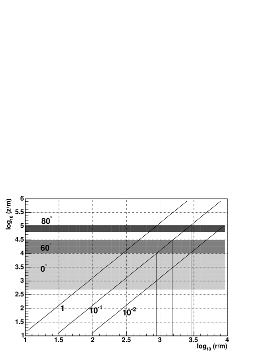
Figure 5: Contour lines for the function $\frac{\delta z}{z}=2\frac{z}{r^{2}}c\delta t$, with $\delta t=12.5$ ns. Different grey bands show the 1-$\sigma$ production distance of muons at different zenith angles.

VI Correlation with angular and core position uncertainties

The method has a third intrinsic limitation because to convert the arrival time histogram into a histogram of production distances using Eq. 36 the incoming direction and the position of shower axis must be known, so that the appropriate values of $r$ can be introduced. In a realistic case these will only be known to a given precision and further uncertainties will arise because of the correlations between both core position and direction uncertainties with the distance distribution obtained. The study of these effects with simulations shows that the reconstructed distributions have a minimum in width when the true shower direction and impact position are used to reconstruct the depth distribution. This adds a interest to the method since it can be used in principle as a further check of the reconstructed directions and impact points.

To study these correlations we explore the stability of the reconstruction to shifts in the core positions and angular directions. Unfortunately the computing time necessary to test such stability can be very large if simulations are used in the same way they were used to test the method in the previous section. We will use instead the results of the muon time delay model of Ref. cazon3 to get distributions of the arrival time for the shower muons from simulated showers. In an attempt to be closer to experimental conditions we assume an array of particle detectors and calculate the number of muons that crosses each of them. We choose 10 $m^{2}~{}\times~{}1.2~{}m$ (area $\times$ height) detectors in a hexagonal grid, separated 1500 m corresponding to the Auger surface detector. This limits the statistics of the reconstructed distribution, $dN/dz$, in a realistic way. Fig. 6 shows an example of the statistics that could be obtained for a $10^{19}$ eV shower with $\theta=60^{\circ}$ and $\phi=90^{\circ}$. ( The azimuth angle $\phi$ was measured counterclockwise respect to East direction.)

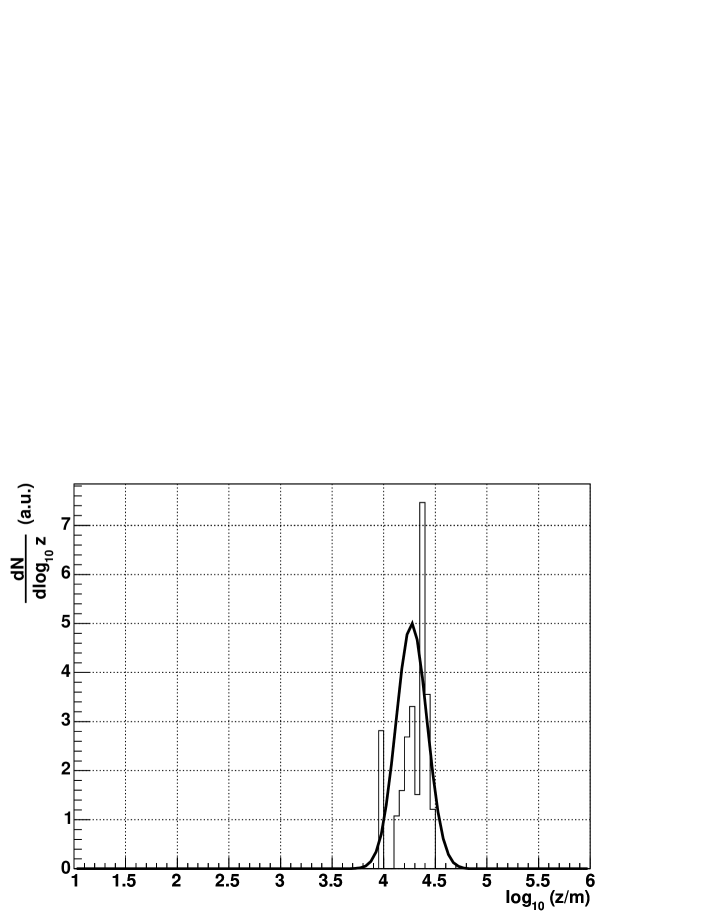
Figure 6: Distribution for a reconstructed $10^{19}$ eV proton shower of $\theta=60^{\circ}$ and $\phi=90^{\circ}$ (histograms) compared with the original distribution when we have finite sampling produced by a finite number of detectors.

We first recalculate the depth distributions assuming that the incidence direction has been misreconstructed by $(\Delta\theta,\Delta\phi)$ with respect to the actual arrival direction chosen for the simulation. This procedure was repeated for different shifts in angular space within an interval of $4^{\circ}\times 4^{\circ}$. For each angular shift both the mean and RMS width of the $z$-distributions in log basis were calculated. In Figs. 7 and 8 representative results showing the mean and RMS width for an example of a $10^{19}$ eV proton shower of $60^{\circ}$ zenith are shown as a function of $\Delta\theta$ ($\Delta\phi$) for fixed $\phi$ ($\theta$), Also the RMS width is shown in a two dimensional plot $(\Delta\theta,\Delta\phi)$ in Fig. 8.

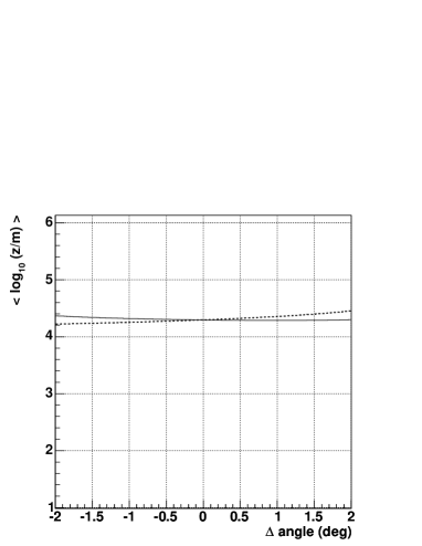
Figure 7: Effects of reconstruction direction shifts for a $10^{19}$ eV proton shower of $\theta=60^{\circ}$ and $\phi=90^{\circ}$ with an $r$ cut $r>1500$ m. Mean of $\log_{10}(z/m)$ as a function of $\Delta\theta$ fixing $\Delta\phi=0$ (dashed line) and as a function of $\Delta\phi$ fixing $\Delta\theta=0$ (continuous line).

It is worth remarking that the mean value of $z$ is quite stable to shifts in azimuthal direction $\Delta\phi$, whereas there is a very slight rise of the reconstructed $z$ when increasing the zenith angle $\theta$. The behavior on this angle in not symmetrical since $\Delta$ introduces an asymmetry between early and late regions. On the other hand the RMS width of the distributions seems to have a local minimum when the correct arrival direction is used. In a typical air shower array the arrival direction is obtained using the relative arrival times of the signals at different locations. The observed minimum of the RMS width of the $z$-distribution suggests that this method could be also used to either reconstruct shower direction independently or, more likely, to check that the reconstruction obtained through conventional methods is consistent with the arrival time of the muons at large distances from shower core, on an individual shower basis.

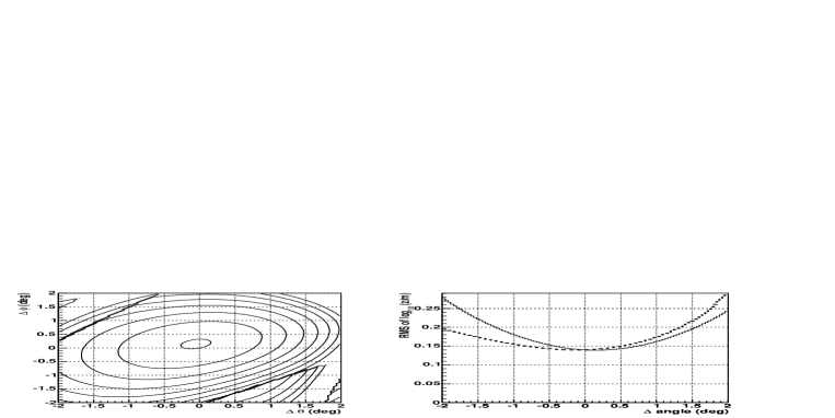
Figure 8: Effects of reconstruction direction shifts in the width of the $z$-distribution for a $10^{19}$ eV proton shower of $\theta=60^{\circ}$ and $\phi=90^{\circ}$ with an $r$ cut $r>1500$ m. Left RMS width of $\log_{10}(z/m)$ as a function of angular shifts $(\Delta\theta,\Delta\phi)$. Right RMS of $\log_{10}(z/m)$ as a function of $\Delta\theta$ fixing $\Delta\phi=0$ (dashed line) and as a function of $\Delta\phi$ fixing $\Delta\theta=0$ (continuous line).

A completely analogous method was followed to study the core position and $z$-reconstruction correlations. The reconstructed impact points were shifted by $(\Delta x,\Delta y)$ in the ground plane with respect to the core of the simulated shower over a grid covering a rectangle of 1000 $\times$ 1000 m. The means and RMS widths for shifts in both $x$ and $y$ positions are shown in Fig. 9. The plots display important discontinuities. They are of statistical nature because the total number of muons in the detector is small and as the core position position is shifted individual detectors are rejected or accepted because of the $r$ cut. The detectors close to the cut are those that have most muons and including or not including them affects the $z$-distribution. These discontinuities are also present in some circumstances for angular shifts because the relative position of the detectors also change but clearly the changes of angular reconstruction modify the distances to shower axis at a second order level. These discontinuities can become smoother by increasing statistics, for instance relaxing the $r$-cut.

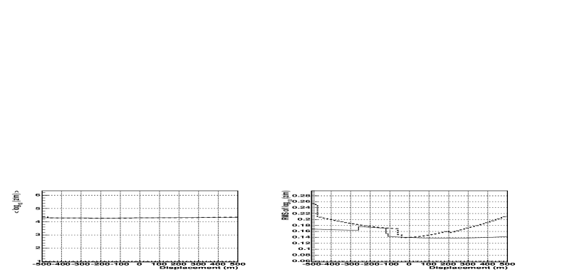
Figure 9: Effects of impact point shifts on the mean (left panel) and RMS (right panel) of the $z$-distribution as a function of $\Delta x$ fixing $\Delta y=0$ (dashed line) and as a function of $\Delta y$ fixing $\Delta x=0$ (continuous line) for a $10^{19}$ eV proton shower at $\theta=60^{\circ}$ and $\phi=90^{\circ}$ with an $r$ cut $r>1500$ m.

Notice that the mean value of $z$ is again quite stable to shifts in core position. This is not difficult to understand since each core location corresponds to a new time-reference plane which is only slightly shifted along the shower axis with respect to the planes obtained for other core positions. The effect is due to the curvature of the front and is therefore a second order effect. The RMS width of the distributions also displays a local minimum when the correct impact point is used. This is also not surprising given that approximately $z\propto r^{2}$. Differences in the $z$ reconstruction arise through the modification of the relative position of the tank with respect to shower core. It can be easily seen that when a tank gets a closer position ($r$ decreases) as a result of the shift, the tanks placed in the opposite $\zeta$ will get to a further one ($r$ increases). This suggests that the width of the reconstructed distribution should have a local minimum when the correct impact point is considered. An example is given relaxing the $r$-cut to 500 m in Figs. 10.

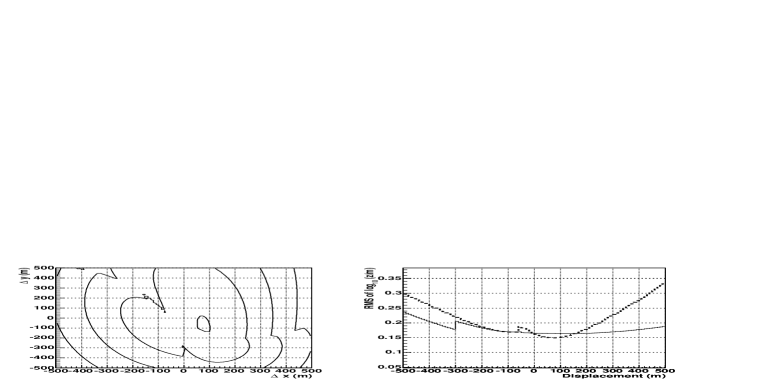
Figure 10: Effects of impact point shifts on the RMS width of the $z$-distribution for a $10^{19}$ eV proton at $\theta=60^{\circ}$ and $\phi=90^{\circ}$ with an relaxed $r$ cut $r>500$ m . Left RMS of $\log_{10}(z/m)$ as a function of a core shift $(\Delta x,\Delta y)$. Right RMS of $\log_{10}(z/m)$ as a function of $\Delta x$ (dashed line) fixing $\Delta y=0$, and as a function of $\Delta y$ fixing $\Delta x=0$ (continuous line).

In a typical air shower array the core position is obtained by the relative amplitude of the signals at different locations either through a fit or by some other means. As for shifts in angular direction the minimum of the RMS width of the $z$-distribution suggests that this method could be used either to reconstruct shower impact points independently or to check that the core position reconstruction obtained through conventional methods is consistent with the arrival time of the muons at large distances from shower core, on an individual shower basis.

VII Summary

We have developed a method that has the potential of reconstructing the production altitude for the muons in inclined cosmic ray showers based on the time distribution of the muon signals in the detectors of an extensive air shower array. This method requires knowledge of the arrival times of muons in the detectors of the air shower array and it can be applied provided that a cut is made in distance to shower axis, $r>r_{c}$. Since the muon signal dominates at high $r$ it can be also used when the detectors cannot separate the muon signal provided that the $r$ cut is chosen so that the muon signal dominates.

The method relies mainly on geometrical arguments and there are minor effects introduced through the kinematical delay of the muons which have little effect at large distances from shower axis. The model does not rely on any assumption about the interaction model for hadrons. Different models would give rise to different kinematic corrections, but the effect is small. Although we have assumed proton showers to explore the viability of this method the method can be also used for heavier nuclei, and similar results would be obtained in that case. The necessary cut introduces limitations because of statistics. We have checked that our method correctly reproduces the depth distribution of muon production using sets of simulated showers with AIRES to a degree of accuracy that is zenith angle dependent. The method works best in the $60^{\circ}-80^{\circ}$ region and it is fairly stable with respect to misreconstruction of the shower core and the incoming direction, in what concerns the mean of the distribution. The RMS width of the production distance distribution however is sensitive to both the reconstructed impact point and arrival direction. The width displays a minimum when the correct impact point and arrival direction are used in the reconstruction procedure.

This work represents a new approach to studying extensive air showers. It will add information concerning the individual development of air showers and can be used to check the reconstructed impact point and arrival directions. The reconstruction of depth development in inclined showers can also have important implications in improving the potential of air shower arrays to detect neutrinos.

VIII Acknowledgments

We thank J Alvarez–Muñiz and A.A. Watson for many discussions on the time structure of shower, and many helpful comments after reading the manuscript. This work was partly supported by the Xunta de Galicia (PGIDIT02 PXIC 20611PN), by MCYT (FPA 2001-3837, FPA 2002-01161 and FPA 2004-01198). We thank CESGA, “Centro de Supercomputación de Galicia” for computer resources.

Appendix A Modelling the distribution of surviving muons

At ground level both muon energies and muon number are reduced because of energy loss and decay. As a first approximation, assuming a constant energy loss per unit depth $dE/dx=-a$ along an uniform atmospheric density $\rho$, both these effects can be easily accounted for. After traveling a distance $l$ a flux of muons $\phi_{0}$ of energy $E_{i}$ reduces by an energy dependent factor to:

$$\phi(l)=\phi_{0}\left[\frac{E_{i}-\rho al}{E_{i}}\right]^{\kappa}.$$ (26)

The last factor takes into account both energy loss and decay in flight. The muon mean lifetime, $\tau$, enters through the exponent $\kappa={mc^{2}/(\rho ac\tau)}\sim 0.8$. We can correct the energy of the produced muons given by Eq. 1 with such factor to obtain the distribution in $E_{i}$, $p_{t}$, $z$ and $\zeta$ after traveling a distance $l$:

$$\frac{d^{4}N(l)}{dz\;\!d\zeta\;\!dE_{i}\;\!dp_{t}}={\cal N}_{0}\;\!\frac{1}{2\pi}\;\!h(z)\;\!f_{1}(E_{i})\;\!f_{2}(p_{t})\left[\frac{E_{i}-\rho al}{E_{i}}\right]^{\kappa},$$ (27)

Here $l$ is the distance traveled by the muon, which enters in Eq. 26, given by $l^{2}=(z-\Delta)^{2}+r^{2}$, where $r$ is the distance to shower axis at the end of the muon trajectory, and $z-\Delta$ is the distance travelled by the muon measured along the shower axis. The correction $\Delta=r\tan\theta\cos\zeta$ relates the distances measured along the axis between the intercepts of shower axis and the muon trajectory with ground level and depends on the zenith angle, $\theta$, as well as on the muon impact point coordinates in the transverse plane, $r$ and $\zeta$.

For a muon to reach ground level there is a minimal production energy given by $E_{i}>mc^{2}+\rho al$. Typical values of $\rho al$ greatly exceed $mc^{2}$, particularly for inclined showers. After traveling a distance $l$ the transverse distance is simply $r=l\sin\alpha$. Performing the change the coordinates from $p_{t}$ to $\sin\alpha$ in Eq. 27 we obtain:

$$\frac{d^{4}N(l)}{dz\;\!d\zeta\;\!dE_{i}\;\!d{\sin{\alpha}}}={\cal N}_{0}\;\!\frac{1}{2\pi}\;\!h(z)\;\!f_{1}(E_{i})\;\!f_{2}\left(\frac{E_{i}}{c}\sin{\alpha}\right)\;\!\left[1-\frac{\rho al}{E_{i}}\right]^{\kappa}\;\!\frac{E_{i}}{c}.$$ (28)

Correlations between the ground variables appear naturally because of energy loss and decay.

We can now introduce the following parameterizations for $f_{1}(E_{i})$ and $f_{2}(p_{t})$ which were shown in cazon3 to give good approximations to the muon time distributions:

$$f_{1}(E_{i})=\frac{\gamma-1}{mc^{2}}\left(\frac{E_{i}}{mc^{2}}\right)^{-\gamma}\Theta(E_{i}-mc^{2}),$$ (29)

$$f_{2}(p_{t})=\frac{p_{t}}{Q^{2}}\exp\left(-\frac{p_{t}}{Q}\right),$$ (30)

where $\gamma\simeq 2.6$ and $Q\simeq 0.17$ GeV/c. Eq. 28 now becomes

$$\frac{d^{4}N}{dz\;\!d\zeta\;\!dE_{i}\;\!d{\sin{\alpha}}}=\frac{{\cal N}_{0}(\gamma-1)}{2\pi}h(z)\;\!\left(\frac{E_{i}}{mc^{2}}\right)^{-\gamma+1}\;\!\frac{E_{i}\sin\alpha}{c^{2}Q^{2}}\exp\left(-\frac{E_{i}\sin\alpha}{cQ}\right)\left[1-\frac{\rho al}{E_{i}}\right]^{\kappa}.$$ (31)

We now integrate the distribution in $E_{i}$ for fixed $z$ and $\alpha$ to obtain:

$$\frac{d^{3}N}{dz\;\!d\zeta\;\!d{\sin{\alpha}}}=\int_{mc^{2}+\rho al}^{\infty}\frac{d^{4}N}{dz\;\!d\zeta dE_{i}\;\!d{\sin{\alpha}}}\;\!dE_{i}={\frac{{\cal N}_{0}(\gamma-1)}{2\pi}}\left(\frac{mc^{2}}{Qc}\right)^{\gamma-1}h(z)\;\!I(l,\sin\alpha)\sin^{\gamma-2}\alpha,$$ (32)

in which $I(l,\sin\alpha)$ is a dimensionless integral in the variable $x=\frac{E_{i}\sin\alpha}{cQ}$:

$$I(l,\sin\alpha)=\int_{y+x_{0}}^{\infty}x^{-\gamma+2}\left[1-\frac{x_{0}}{x}\right]^{\kappa}\exp\left(-x\right)dx,$$ (33)

with $x_{0}(l,\alpha)=\frac{\rho al}{cQ}\sin\alpha$ and $y(\alpha)=\frac{mc^{2}}{cQ}\sin\alpha$. We note that $y\ll x_{0}$ when $l\gg mc^{2}/\rho a\simeq 500$ m and in that case the integral can be approximated replacing its lower limit by $x_{0}$. Since $z$, the distance of muon production, is relatively large, particularly for inclined showers, this approximation is adequate for most circumstances. Then it is easily seen that the integral depends only on the combination $l\sin\alpha=r$, i.e. on the transverse distance. We can then replace $I(l,\sin\alpha)$ by $I(r)$.

In terms of the differential solid angle $d^{2}\Omega=-d\zeta d\cos\alpha$ the number of muons arriving at ground level coming from production distance $z$ becomes:

$$\frac{d^{3}N(r)}{dz\;\!d^{2}\Omega}=-\frac{d^{3}N(r)}{dz\;\!d\zeta\;\!d\cos\alpha}=\frac{{\cal N}_{0}(\gamma-1)}{2\pi}\left(\frac{mc^{2}}{Qc}\right)^{\gamma-1}h(z)~{}I(r)\left(\frac{\cos\alpha}{\sin\alpha}\right)\sin^{\gamma-2}\alpha.$$ (34)

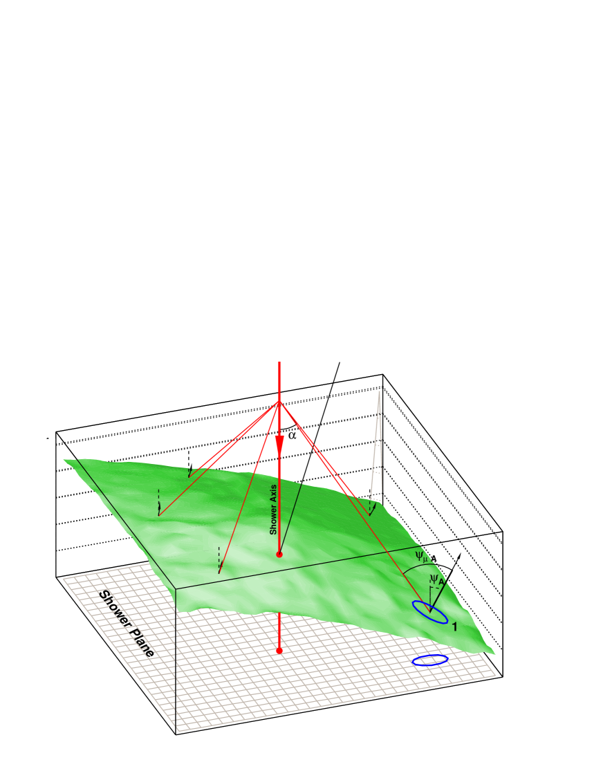
Figure 11: Illustration of the relation between the ground surface, the transverse plane (shower plane) and the shower axis (big arrow). The small arrows represent a detector surface direction normal to the detector surface, the dashed lines are parallel to shower axis and the continuous lines are the muon trajectories. The expressions for number of muons $dN_{A}$ which go through the surface element $d^{2}A$ (labeled 1) are described in the text.

Using the relations between $z$, $l$ and $\alpha$, we can substitute Eq. 34 into Eq. 6 and integrate in $z$ to obtain:

$$\hat{N}_{Ar\zeta}\equiv\frac{1}{r}\;\!\frac{d^{2}N_{A}}{dr\;\!d\zeta}=\frac{{\cal N}_{0}(\gamma-1)}{2\pi}\left(\frac{mc^{2}}{Qc}\right)^{\gamma-1}~{}\frac{I(r)}{r}~{}\int h(z)\;\!\frac{\cos\alpha~{}D_{A}(\Omega)\sin^{\gamma-2}\alpha}{l}dz.$$ (35)

$\hat{N}_{Ar\zeta}$ is the number of muons going through $d^{2}A$ (whose projection onto the transverse plane is $rdrd\zeta$) and has a non-trivial geometrical dependence through the $D_{A}(\Omega)$ factor. This factor can be both greater or less than 1 and becomes 1 as the angle $\alpha$ tends to zero, that is in the limit of small $r$. In that case $\hat{N}_{Ar\zeta}$ simply becomes the muon surface density in the transverse plane. $D_{A}(\Omega)$ can be regarded as a geometrical correction which accounts for the fact that the muons do not travel parallel to the shower axis and the fact that the detector planes are not perpendicular to the shower axis not to the muon fluxes (See Fig. 11).

It can be shown that when $z$ and $r$ are fixed $D_{A}$ depends on the angle $\zeta$ because the angles $\alpha$ and $\psi_{\mu A}$ differ. As a result the factor $D_{A}$ is responsible for part of the asymmetry in the muon signal. For instance a horizontal surface will have larger efficiency for collecting early arriving muons because $\psi_{\mu A}$ is smaller than for late arriving muons. Note that $D_{A}(\Omega)$ would be exactly 1 for an “ideal” detector of spherical shape. In that case these differences disappear.

The expression obtained in Eq. 10 relates the time distribution to a transform of the depth distribution $h(z)$ which effectively accounts for muon decay in flight through $l$. If we are interested in obtaining the production distribution $h(z)$ formally we can rewrite Eq. 10 as:

$$h(z)=g(t)\frac{dt}{dz}l^{-1+\gamma}\cos^{-1}\alpha~{}D_{A}^{-1}(\Omega)\int_{0}^{\infty}h(z)\;\!{l}^{1-\gamma}\cos\alpha~{}D_{A}(\Omega)dz.$$ (36)

This expression in principle allows us to obtain $h(z)$ from the time distribution of the arriving muons at a given point on the ground, $g(t)$. On its own it is not very useful because typically a single detector in an air shower array does not collect sufficient statistics to sample $h(z)$ reliably. in a practical situation one must combine the results of several detectors. Since $h(z)$ is normalized to 1, the unknown factor which is given by the integral on the RHS of the equation acts as an effective weight to be given to each detector. In a first attempt it is possible to ignore it. For inclined showers the weights to be applied for the relevant detectors are expected to be quite similar and the approximation works well. More sophisticated approaches could be deviced for instance using Eq. 36 with a trial $h(z)$ function in an iterative process to sample $h(z)$. However since $h(z)$ is not directly available from the simulation program used we will not need to calculate $h(z)$ and we have instead compared our results to the $z$-distribution of the surviving muons.

Appendix B Parameterization of kinematical delays

The mean kinematical time delay can be obtained by applying the method developed in Ref. cazon3 , summarized in Eq 16 to the distributions discussed in this article:

$$<t_{\varepsilon}>\ =\frac{\int t_{\varepsilon}\frac{d^{4}N}{dz\;\!d\zeta\;\!dE_{i}\;\!dr}dE_{i}}{\int\frac{d^{4}N}{dz\;\!d\zeta\;\!dE_{i}\;\!dr}dE_{i}}.$$ (37)

After some manipulation, using the results of the models in Appendix A a simple expression can be obtained for it:

$$<t_{\varepsilon}>\ =\ \frac{1}{2c}\frac{r^{2}}{l}{\left(\frac{mc^{2}}{cQ}\right)^{2}}\frac{\int_{y+x_{0}}^{\infty}x^{-\gamma}\left[1-\frac{x_{0}}{x}\right]^{\kappa-1}\exp\left(-x\right)dx}{\int_{y+x_{0}}^{\infty}x^{-\gamma+2}\left[1-\frac{x_{0}}{x}\right]^{\kappa}\exp\left(-x\right)dx}=\frac{1}{2c}\frac{r^{2}}{l}\epsilon(r,z-\Delta),$$ (38)

with $x_{0}(l,\alpha)=\frac{\rho al}{cQ}\sin\alpha$ and $y(\alpha)=\frac{mc^{2}}{cQ}\sin\alpha$.

In the last equality of the above expressions we have introduced the dimensionless factor $\epsilon(r,z-\Delta)$. We note that for $z-\Delta\gg r$, for instance in inclined showers, it gives the ratio of the average kinematical delay to the geometrical delay at a given position $\frac{<t_{\varepsilon}>}{t_{g}}\simeq\epsilon(r,z-\Delta)$. This indicates the regions where the geometric delay dominates, which depend on production distance. For practical purposes we have parameterized $\epsilon(r,z)$ as follows:

$$\epsilon(r,z)=p_{0}(z)\left(\frac{r}{\rm m}\right)^{p_{1}},$$ (39)

with

$$\log_{10}p_{0}(z) = -0.6085+1.955\ \log_{10}(z/m)-0.3299\ \log^{2}_{10}(z/m)+0.0186\ \log^{3}_{10}(z/m),$$ (40)

$$\log_{10}p_{1} = -1.176.$$ (41)

References

- (1) J. Linsley and L. Scarsi, Phys. Rev. 128 (1962) 2384.
- (2) J. Lapikens, PhD Thesis, University of Leeds, 1974
- (3) A. A. Watson and J. G. Wilson J. Phys. A: Math. Nucl. Gen. 7 (1974) 1199; R. Walker and A. A. Watson, J. Phys. G 7 (1981) 1297; R. Walker and A. A. Watson, J. Phys. G 8 (1982) 1131.
- (4) T. Antoni et al., Astropart. Phys. 18 (2003) 319. [arXiv:astro-ph/0204266].
- (5) Nagano and A.A. Watson, Rev. Mod. Phys. 72 (2000) 689.
- (6) J. Abraham et al., [Auger Collaboration], Nucl. Instr. Meth. A 523 (2004) 50.
- (7) T.A. Danilova, D. Dumora, A.D. Erlykin, and J. Procureur J. Phys. G: Nucl. Part. Phys. 20 (1994) 961.
- (8) I. M. Brancus, B. Vulpescu, H. Rebel, M. Duma and A. A. Chilingarian, Astropart. Phys. 7 (1997) 343.
- (9) L. Pentchev, P. Doll, and H.O. Klages, J. Phys. G: Nucl. Part. Phys. 25 (1999) 1235.
- (10) M. Ambrosio et al., Proc. of the 26th Int. Cosmic Ray Conference, Salt Lake City, Utah, 17-25 Aug 1999, vol 5, p. 312.
- (11) M. Ave, R.A. Vázquez, and E. Zas, Astropart. Phys. 14 (2000) 91.
- (12) L. Cazón, R.A. Vázquez, A.A. Watson, and E. Zas, Astropart. Phys. 21 (2004) 71.
- (13) J. Alvarez–Muñiz and I. Valiño, in preparation.
- (14) S. J. Sciutto, AIRES: A System for Air Shower Simulation, Proc. of the 26th Int. Cosmic Ray Conference, Salt Lake City, Utah, 17-25 Aug 1999, vol. 1, p. 411; S. J. Sciutto astro-ph/9911331.
- (15) M. Ave, J.A. Hinton, R.A. Vázquez, A.A. Watson, and E. Zas Phys. Rev. D 65 (2002) 063007.
- (16) The Pierre Auger Project Design Report. By Auger Collaboration. FERMILAB-PUB-96-024, Jan 1996. (www.auger.org).
- (17) E. J. Fenyves et al., Phys. Rev. D 37 (1988) 649; C. Forti, et al., Phys. Rev. D 42 (1990) 3668.