Pulsar Physics at Low Frequencies

J. A. Eilek¹, T. H. Hankins¹ and A. Jessner²

Abstract

Recent work has made it clear that the “standard model” of pulsar radio emission cannot be the full answer. Some fundamental assumptions about the magnetic field and plasma flow in the radio-loud region have been called into question by recent observational and theoretical work, but the solutions to the problems posed are far from clear. It is time to formulate and carry out new observational campaigns designed to address these problems; sensitive low-frequency observations will an important part of such a campaign. Because pulsars are strong at low frequencies, we believe there will be a good number of candidates even for high-time-resolution single pulse work, as well as mean profile and integrated spectrum measurements. Such data can push the envelope of current models, test competing theories of the radio loud region, and possibly provide direct measures of the state of the emitting plasma.

¹ New Mexico Tech, Socorro NM 87801 USA

² Max-Planck Institut für RadioAstronomie, Bonn, Germany

1. Introduction

Pulsar radio emission is not well understood. Much current work is grounded in standard models and assumptions about the geometry of the emitting region and about the nature and dynamics of the plasma therein. While these models work well for some stars, we now know they fail for others. It has become clear from recent work that specific predictions of this model are not always met in real stars, and that important assumptions within the model may be inconsistent with the data. Thus, while the standard model of the pulsar magnetosphere has served us well, it now seems time to revisit it critically, with a careful eye to what the data tell us about the physics in the radio emission region.

We think that the most fruitful research is the study of just those stars in which the standard model fails seriously. These will be the stars that reveal the most about conditions in the emission region, and help us to formulate the next generation of models. In addition, the high quality of modern pulsar data acquisition systems justifies renewed observational effort: what observations can be carried out which will guide and critically test the models?

Because pulsar emission shows strong frequency evolution, low frequency observations are an important part of the answer. However, although pulsars are strong at low frequencies, good data below $100$ MHz are hard to come by. The LWA thus comes at an opportune time. In this paper, we discuss some areas in which the standard model fails, and then describe three types of low-frequency experiments which will be important in developing and testing the next generation of pulsar models.

2. The Pulsar Setting

A “standard model” of a pulsar’s magnetosphere has been developed from early observations and theoretical work. A rapidly rotating neutron star supports a strong, misaligned, dipolar magnetic field. The plasma-filled magnetosphere corotates with the star, except in the open field line region where the star’s magnetic fields connect to the universe beyond the light cylinder. Plasma in this open field line region (somehow) emits coherent radio emission; we observe “pulses” when the star’s rotation sweeps this forward-beamed emission region past our line of sight.

While this picture is very likely true in general, the devil can be in the details. For example, two interesting results which relate particularly to low frequency observations have emerged from our recent work. We now know the geometry of the emission region is more complex in many stars than had been thought. We also strongly suspect that the plasma in the emission region is much less dense than had been assumed, and thus must be highly turbulent.

2.1. Geometry in the Radio Emission Region

A fundamental assumption of the standard model is that a strong, dipolar magnetic field dominates the plasma dynamics in the radio emission region. This picture makes specific, quantitative predictions. One prediction involves the rotation of the linear polarization angle as the emission beam sweeps past the observer’s sight line. Another involves the mean emission profile: we should only detect radio emission when the line of sight intersects open field lines.

In addition, the standard model now includes frequency evolution of the mean profile, based on trends observed in many stars. For instance, “radius to frequency mapping” says lower-frequency profiles should be broader; this may connect to density stratification in the emission region. Or, profiles should evolve from “cone” emission at high frequencies to “core” emission at low frequencies; this may reflect different plasma states or emission mechanisms in different parts of the open field line region.

These predictions are not always borne out by the data. We gathered time-aligned mean profiles and high-quality polarimetry, and used these data to study the geometry of the emission region in 52 bright pulsars (Hankins & Rankin 2005, Eilek & Hankins 2005). We did, indeed, verify that the standard picture works in about half of the stars — but in the other half it does not. Many stars show complex frequency-dependent changes in their mean emission profile, which do not follow the trends predicted by the standard model. Some stars even show emission at rotation phases which cannot arise from open field lines in a simple dipole geometry. In addition, many stars show striking deviations from the position angle behavior predicted for a pure dipole magnetic field in the emission region. These deviations can be steady in some stars, fluctuating in others, and can change with observing frequency. Other stars show evidence that the magnetic field switches between two different, quasi-stable states, which is impossible if the magnetic field is a static dipole.

2.2. Plasma Density in the Radio Emission Region

Another fundamental assumption in the standard model is that the charge density of the radio-loud plasma is exactly that needed to shield the rotation-induced electric field, and thus to allow the plasma magnetosphere to corotate smoothly with the star (after Goldreich & Julian 1969). It follows that the plasma in the radio emission region would be undergoing smooth, coasting flow. This assumption is attractive in that it simplifies the modelling; but it seems to be inconsistent with the fact that we observe pulsars at low radio frequencies.

The connection between plasma density and observing frequency comes from the coherent emission mechanism. Nearly all coherent plasma emission processes operate at the local (comoving) plasma frequency, which depends on the local number density of the plasma (e.g., Kunzl et al. 1998). Our recent observations of the pulsar in the Crab Nebula support this hypothesis. The radio emission in this pulsar is narrow-band $(0.1<\Delta\nu/\nu<1$ ) and comes in bursts of very short duration (unresolved at 2 nanoseconds; Hankins et al. 2003). These observations are consistent with both the bandwidth and the timescales predicted by Weatherall’s numerical simulations (1997, 1998) of radio emission from collapsing solitions in strong plasma turbulence, but they are inconsistent with the timescales predicted by competing models of the emission mechanism. It therefore seems likely that strong plasma turbulence creates coherent radio emission in the Crab pulsar.

If plasma emission is indeed the emission mechanism in pulsars, we can directly determine the density (in the star’s frame) of the emitting plasma (with some dependence on the streaming speed of the plasma; we follow modern models which find $\gamma\sim 10^{2}$ - $10^{3}$ , e.g. Arendt & Eilek 2002). This exercise tells us that the density of the plasma emitting at, say, 1 GHz or 100 MHz is far below that needed for smooth corotation. This fact has two important consequences.

(1) High and low frequency emission must originate in different parts (high and low density) of the radio-loud region. In some stars these regions may be stratified in altitude (consistent with radius-to-frequency mapping in their mean profiles), but in other stars the high and low density regions appear to coexist — as would be the case in a highly turbulent plasma.

(2) The rotation-induced electric field cannot be fully shielded. The plasma must be subject to strong local forces, and is probably in a highly unsteady, turbulent state. The lower the density, the more unsteady the plasma should be. Because dynamical timescales in this system are on the order of microseconds, we suspect this unsteady plasma flow is the cause of microstructure, which exists in many stars and is especially strong at low frequencies.

3. Low Frequency Experiments We Would Like to See

Broad frequency coverage is crucial to testing theoretical models, because the characteristics of pulsar radio emission can change dramatically between 100 MHz and 10 GHz, and because different frequencies are emitted by different parts of the radio-loud plasma. In fact, if our hypothesis of radio emission from strong plasma turbulence is correct, the strongest discrepancies between data and models should arise at low frequencies. We describe three types of pulsar observations which address these problems and which we hope could be carried out with the LWA.

3.1. Integrated Pulsar Spectra

Time-integrated pulsar fluxes are the easiest experiment to do, because the stars are bright at low frequencies (as in Figure 1). The spectrum of some stars turns over well above 100 MHz, while that of others continues rising to the lowest observable frequencies.

Refer to caption — Figure 1.: Integrated spectra of three bright pulsars, from Malofeev et al. (1994). The spectrum of some pulsars continues to rise to the lowest observed frequencies, while others turn over at several hundred MHz. There is as yet no good understanding of these spectra.

The integrated spectra are among the hardest data to interpret, because of the lack of robust spectral predictions by different emission models. Nonetheless, we suggest that probing the spectrum and frequency range of such emission can be important as a constrant on, or test of, future models. This will require LWA-derived fluxes to be be combined with higher-frequency data from other telescopes to determine broad-band integrated spectra of a large number of stars. For instance, models need to address questions such as what sets the spectral range of the coherent emission? Why does the spectrum turn over at low frequency? Is it a spatial scale (which could limit maser growth, for instance)? Is it a lack of plasma at the right density, or a lack of turbulent drivers in that plasma (either of which could limit plasma turbulent emission)?

3.2. Mean Profiles

The mean profile reveals the structure of the emission region. It tells us about the geometry and density structure in the region, as well as the local magnetic field (which is revealed through its polarization signature). When a broad frequency range can be studied, the mean profiles in many stars turn out to show strong frequency evolution, as illustrated in Figure 2. As we noted above, the data often disagree with what the standard model predicts.

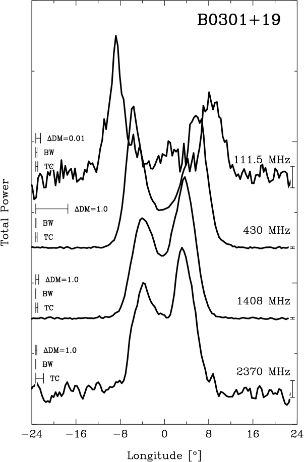
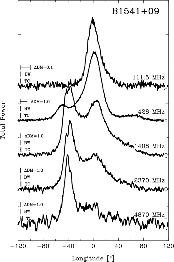
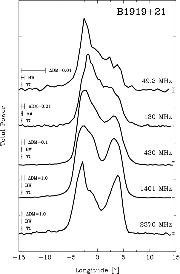
In order to understand the pulsar emission geometry in the important, “non-standard” stars, we need high quality mean profiles with polarization information. We also need the broadest possible frequency range, which can be reached by combining LWA data with higher-frequency data from other telescopes. Once again, such data will be important to lead and test future models. For instance, does the emission geometry of the star change at frequencies below the spectral break? Why do some pulsars become strongly linearly polarized at low frequencies, and does the emission geometry change with the polarization? How often does the linear polarization direction change with frequency (which should not happen at all in the standard model)?

Because the pulsar signal can be integrated synchronously to form the final profile, we anticipate that many stars will be bright enough to be studied with milliperiod resolution at good S/N. We do note that some stars will be too strongly broadened by interstellar scintillation at these low frequencies; but dispersion measure is a rough measure of turbulent broadening (e.g., Löhmer et al. 2004), and quite a few stars have sufficiently low dispersion to be profitably studied even at tens of MHz.

3.3. Single Pulse Studies

This is the most challenging experiment but it will be worth the effort. Single pulse studies at high time resolution tell us about the time dependence of the plasma — as reflected in such phenomena as microstructure, rapid polarization fluctuations and drifting subpulses. As we have emphasized before, studies over a broad frequency range are needed to understand a star and test the models. Low frequencies are particularly interesting here, because microstructure and subpulses tend to be stronger at low frequencies, where we would expect the density imbalance and plasma dynamics to be the most noticable.

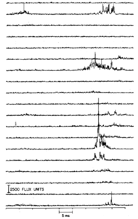
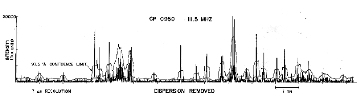
Observations such as these have potentially high payoff, because they come closest to predictions that can be made by theoretical models of the emission region. They will be difficult at low frequencies, however, because sub-millisecond time resolution is necessary which makes sensitivity and scattering broadening important issues. We believe a good number of bright puslars will be observable in this mode. By current estimates, the LWA will have thermal noise $\mathrel{\hbox{\hbox to0.0pt{\hbox{\lower 4.0pt\hbox{$\sim$}}\hss}\hbox{$<$}}}1$ mJy in one hour’s integration, around the middle of its frequency range. This scales to $\mathrel{\hbox{\hbox to0.0pt{\hbox{\lower 4.0pt\hbox{$\sim$}}\hss}\hbox{$<$}}}3$ Jy for millisecond time resolution; so single pulse work at high S/N can only be done on pulsars as bright as, say, 300 Jy. While this is large compared to the time-integrated flux for most pulsars, our experience is that many pulsars show occasional very bright microbursts. Figure 3 shows two examples, each of which become brighter than 10 kJy for brief moments, and thus easily detectable in a triggered observation.

4. Closing comments

There is much still to be learned about the physics of pulsar radio emission. New observations have made it clear that the simple model, which has been around nearly since pulsars were discovered, does not supply all the answers. We hope that the data to come from new instruments can inspire a new understanding of the physics, not to mention closer contact between observers and theorists.

Low-frequency information is particuarly important here. Although the LWA has been envisioned primarily as an imaging instrument, it can also make important contributions to pulsar science, by providing critical low-frequency information which is not easily available anywhere else.

Acknowledgments.

We thank Don Backer and Frazer Owen for technical discussions, and the members of the Socorro pulsar group for ongoing discussions on pulsar physics. This work was partly supported by NSF grant AST-0139641.

References

Arendt, P. N. Jr. & Eilek, J. A., 2002, ApJ, 581, 451

Eilek, J. A. & Hankins, T. H., 2005, submitted to ApJ

Goldreich, P. & Julian, W. H., 1969, ApJ, 157, 869

Hankins, T. H., 1971, Ph.D. thesis, University of California at San Diego

Hankins, T. H., Kern, J. S., Weatherall, J. C. & Eilek, J. A., 2003, Nat, 422, 141

Hankins, T. H. & Rankin, J. M., 2005, submitted to ApJ

Kunzl, T., Lesch, H., Jessner, A. & von Hoensbroech, A., 1998, ApJ,, 505, L139

Löhmer, O., Mitra, D., Gupta, Y., Kramer, M. & Ahuja, A., 2004, A&A, 425, 569

Malofeev, V. M., Gil, J. A., Jessner, A., Malof, I., Sieber, W. & Wielebinski, R., A&A, 368, 230

Weatherall, J. C., 1997, ApJ, 483, 402

Weatherall, J. C., 1998, ApJ, 506, 341