Stochastic Gravitational Wave Background from Cosmological Supernovae

Abstract

Based on new developments in the understanding of supernovae (SNe) as gravitational-wave (GW) sources we estimate the GW background from all cosmic SNe. For a broad range of frequencies around 1 Hz, this background is crudely comparable to the GW background expected from standard inflationary models. While our estimate remains uncertain within several orders of magnitude, the SN GW background may become detectable by second-generation space-based interferometers such as the proposed Big-Bang Observatory (BBO). By the same token, the SN GWs may become a foreground for searches of the inflationary GWs, in particular for sub-Hz frequencies where the SN background is Gaussian and where the BBO will be most sensitive. SN simulations lasting far beyond the usual cutoff of about 1 s are needed for more robust predictions in the sub-Hz frequency band. An even larger GW background can arise from a hypothetical early population of massive stars, although their GW source strength as well as their abundance are currently poorly understood.

I Introduction

Core-collapse supernova (SN) explosions are among the most violent astrophysical phenomena. The total energy of about $3\times 10^{53}~{}{\rm erg}$ is primarily released in a neutrino burst lasting for a few seconds. About 1% goes into the actual explosion while only a fraction of about $10^{-4}$ is emitted in visible light, yet a SN can outshine its host galaxy. In addition, SNe are expected to be strong gravitational-wave (GW) sources. About 1 SN per second takes place in the visible universe, but the neutrino burst has been observed only once from SN 1987A, the closest SN in modern history. GWs are even more difficult to detect and have never been measured from any source. On the other hand, the next galactic SN probably will be observed with high statistics in several large neutrino detectors as well as with the existing GW antennas. For the first time there is a realistic opportunity to observe such a cataclysmic event in all forms of radiation.

However, galactic SNe are rare so that the next SN neutrinos to be observed could well be the diffuse neutrino background from all cosmic SNe. The limit from Super-Kamiokande Malek:2002ns already touches the upper range of theoretical predictions Strigari:2003ig ; Ando:2004hc ; Strigari:2005hu . The proposed gadolinium upgrade Beacom:2003nk or a corresponding future megatonne detector may well produce a positive detection. Therefore, it is natural to ask the analogous question whether the diffuse GW background from all past cosmic SNe will be important for current or future GW antennas that search for signals from individual astrophysical events or for the stochastic cosmic background that probably arises in the very early universe during the inflationary epoch.

The existing literature focuses on GWs from the SN bounce signal in the kHz range that is relevant for bar detectors or ground-based laser interferometers such as LIGO, VIRGO, GEO and TAMA. However, recent studies of SNe as GW sources indicate that a much stronger signal may be expected from the large-scale convective overturn that develops in the delayed explosion scenario during the epoch of shock-wave stagnation that may last for several 100 ms before the actual explosion Mueller:2003fs ; Fryer:2004wi . Moreover, the relevant frequencies reach below 1 Hz where they may be relevant for space-based detectors. While we find that a first-generation instrument such as LISA is not sufficient, the GW background from SNe may become relevant for a second-generation detector such as the proposed Big-Bang Observatory (BBO).

While a detection of the GW background from SNe would be intriguing from the perspective of SN physics, particularly in conjunction with a future detection of the corresponding neutrino background, this possibility could be a significant problem for searches of the inflationary GW background that would probe a very early epoch of the universe. In fact, if ordinary astrophysical foreground sources were seriously expected to mask the inflationary GWs in some range of frequencies, probably an instrument like the BBO should be designed to have its optimal sensitivity in a different frequency range. Therefore, a reliable understanding of such foregrounds is an important task in view of the long-term perspective of observing the big bang in GWs.

We begin our study in Sec. II with a general expression for the GW background from all cosmic SNe. In Sec. III we consider core-collapse SNe as sources, whereas in Sec. IV we turn to an early population of massive stars. In Sec. V we estimate the frequency range where the GW background is Gaussian before concluding in Sec. VI. We always use natural units with $\hbar=c=1$.

II Estimating the Gravitational Wave Background

We assume all SNe are identical GW sources defined by the Fourier transform $\tilde{h}(f)\equiv\int_{-\infty}^{+\infty}dt\,e^{-i2\pi ft}h(t)$ of the dimensionless strain amplitude $h(t)$, which is proportional to deviations from spherical symmetry of the energy-momentum tensor. In general, $h(t)$ is obtained from numerical simulations. However, the contribution of asymmetric neutrino emission is explicitly Epstein:1978dv ; mueller2

$$h(t)=\frac{2G_{\rm N}}{D}\int_{-\infty}^{t-D}dt^{\prime}\,L_{\nu}(t^{\prime})q(t^{\prime})\,,$$ (1)

where $G_{\rm N}$ is Newton’s constant, $D$ the distance to our “standard SN,” and $L_{\nu}(t)$ the neutrino luminosity. Further, $q(t)\leq 1$ is an asymmetry parameter defined as the angle-dependent neutrino luminosity folded over an angular function; for details see Eqs. (27)–(29) in Ref. mueller2 .

Equation (1) shows that $h(t)$ converges to a constant value $h_{\infty}$ for $t\gtrsim t_{e}$, with $t_{e}$ the neutrino emission time scale of a few seconds. Therefore, the neutrino burst causes $h(t)$ to jump from zero to a non-vanishing constant value, an effect called the “burst with memory” Smarr:1977fy ; Epstein:1978dv ; Turner:1978jj ; gw_memory ; Burrows:1995bb . We now write

$$2\pi f\,\tilde{h}(f) = -i\int_{-\infty}^{+\infty}dt\,e^{-i2\pi ft}\,\dot{h}(t)$$ (2)

$$\simeq -i\frac{2G_{\rm N}}{D}\,\int_{-\infty}^{+\infty}dt\,L_{\nu}(t)q(t)\,,$$

where in the second step we used Eq. (1) and assumed $f\ll(2\pi t_{e})^{-1}$, which is known as the zero-frequency limit Smarr:1977fy ; Epstein:1978dv ; Turner:1978jj ; bontz_price . This implies

$$f|\tilde{h}(f)| \simeq \frac{|h_{\infty}|}{2\pi}=\frac{G_{\rm N}}{\pi D}\left\langle q\right\rangle E_{\nu}$$

$$\simeq 2.6\times 10^{-19}\,\left\langle q\right\rangle\left(\frac{10\,{\rm kpc}}{D}\right)\left(\frac{E_{\nu}}{3\times 10^{53}\,{\rm erg}}\right)\,,$$

where $E_{\nu}=\int_{-\infty}^{+\infty}dt^{\prime}\,L_{\nu}(t^{\prime})$ is the total emitted neutrino energy and $\left\langle q\right\rangle\equiv\int_{-\infty}^{+\infty}dt^{\prime}\,L_{\nu}(t^{\prime})q(t^{\prime})/E_{\nu}$ is the luminosity-weighted average neutrino anisotropy. Although the zero-frequency limit Eq. (II) is valid for $f\ll(2\pi t_{e})^{-1}$, we will use it to evaluate the GW signal at $f\lesssim(2\pi t_{\rm sim})^{-1}$, where $t_{\rm sim}<t_{e}$ is the maximal simulation time (less than a second), and then we continuously extend $|\tilde{h}(f)|$ to lower frequencies. Current simulations do not cover the strain spectrum below fractions of a Hertz.

The energy density in GWs at frequency $f$ per logarithmic frequency interval in units of the cosmic critical density $\rho_{\rm c}=3H_{0}^{2}/(8\pi G_{\rm N})$ can be written as Phinney:2001di

$$\Omega_{\rm gw}(f)=\frac{16\pi^{2}D^{2}}{15G_{\rm N}\rho_{\rm c}}\int_{0}^{\infty}dz\,\frac{R_{\rm SN}(z)}{1+z}\left|\frac{dt}{dz}\right|f_{z}^{3}\left|\tilde{h}(f_{z})\right|^{2}\,,$$ (4)

where $R_{\rm SN}(z)$ is the SN rate per comoving volume, $f_{z}\equiv(1+z)f$, and $\tilde{h}(f)$ is the strain spectrum of an individual SN at distance $D$. The cosmological model enters with $|dt/dz|=[(1+z)H(z)]^{-1}$ and, for a flat geometry,

$$H(z)=H_{0}\left[\Omega_{\rm M}(1+z)^{3}+\Omega_{\Lambda}\right]^{1/2}\,.$$ (5)

We will use the parameters $\Omega_{\rm M}=0.3$, $\Omega_{\Lambda}=0.7$, and $H_{0}=h_{0}\,100~{}{\rm km}~{}{\rm s}^{-1}~{}{\rm Mpc}^{-1}$ with $h_{0}=0.72$.

The SN rate as seen from Earth is

$$\int_{0}^{\infty}dz\,\frac{R_{\rm SN}(z)}{1+z}\frac{dV}{dz}=\int_{0}^{\infty}dz\,R_{\rm SN}(z)\frac{4\pi r^{2}(z)}{(1+z)H(z)}\,,$$ (6)

where $dV/dz$ is the fractional volume element, the cosmic expansion rate at redshift $z$ is given by Eq. (5), and $r(z)$ is the comoving coordinate, $dr=(1+z)dt$.

III Supernovae

The cosmic star-formation rate and, as a consequence, the core-collapse SN rate is reasonably well known at redshifts $z\lesssim 5$ Daigne:2004ga , but becomes rather uncertain at larger $z$. The SN rate per comoving volume is often expressed as

$$R_{\rm SN}(z)=R_{\rm SN}^{0}\times\left\{\begin{array}[]{ll}(1+z)^{\beta}&\mbox{for $z<1$}\\ 2^{\beta-\alpha}(1+z)^{\alpha}&\mbox{for $1\leq z\leq 20$}\end{array}\right..$$ (7)

If not otherwise stated, we will use $\beta=2.7$, $\alpha=0$, and the present-day rate $R_{\rm SN}^{0}=2\times 10^{-4}\,{\rm Mpc}^{-3}\,{\rm yr}^{-1}$. These values are consistent with the Super-K limits on the diffuse neutrino background Malek:2002ns . The parameter $0\lesssim\alpha\lesssim 2$ is much less constrained than $\beta$ and $R_{\rm SN}^{0}$ because $\alpha$ influences the rate only for $z>1$ where the neutrinos are redshifted below the Super-K threshold Strigari:2003ig ; Ando:2004hc ; Strigari:2005hu . This situation may change if low-threshold detectors such as the gadolinium upgrade of Super-K Beacom:2003nk become operative.

For the strain spectrum $\tilde{h}(f)$ of an individual event we first use the recent 3-dimensional asymmetric simulation shown in Fig. 9 of Ref. Fryer:2004wi . We plot in Fig. 1 the resulting GW background together with an estimate scaled downward by a factor of 100. The latter GW background with a total energy released in GWs of about $8\times 10^{-11}\,M_{\odot}$ should be considered more realistic Fryer:2004wi . We also show sensitivities of LISA, BBO bbo , LIGO (or EGO) correlated third generation AB:2002 , and the ultimate DECIGO Seto:2001qf , which would be a quantum limited space-based interferometer with mirror masses of 100 kg. For some frequencies, our lower estimate for the GW background from SNe can be comparable to the most optimistic GW background from slow-roll inflation (horizontal lines).

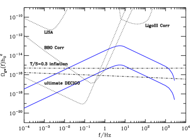
Figure 1: Spectrum of GW background from Eq. (4) for a simulation from Ref. Fryer:2004wi . Solid lines: the spectrum is continuously extended with the low-$f$ tail according to Eq. (II). The upper curve is obtained from Fig. 9 of Ref. Fryer:2004wi , whereas the lower is the same shifted downwards by a factor 100, which is considered a more realistic estimate. Horizontal lines: GW stochastic spectrum produced during slow-roll inflation and evaluated from Eq. (6) of Ref. Turner:1996ck . We assume $T/S=0.3$ for the ratio of the tensorial and scalar contributions to the cosmic microwave background radiation (CMBR) anisotropy and consider two values $\pm 10^{-3}$ of the running of the tensorial power-law index. Dotted lines: sensitivities of the indicated detectors. The BBO sensitivity is approximate and may change slightly in the final design.

Next, we use the three models s15r, s11nr180, and pns180 from recent two-dimensional (2D) core-collapse simulations based on a detailed implementation of spectral neutrino transport or following the long-time evolution of the newly born neutron star with good resolution, respectively Mueller:2003fs . Models s15r and s11nr180 are fully 2D, i.e. axially symmetric, stellar core collapse and SN simulations of a rotating 15$\,M_{\odot}$ and a non-rotating 11.2$\,M_{\odot}$ star with very strong core convection after shock formation. Convection takes place both in the neutrino-heated postshock layer and inside the nascent neutron star Buras:2003 ; Janka:2004jb . The simulations were done with a full spectral treatment of neutrino transport and neutrino-matter interactions with gravitational redshift effects taken into account. An approximation to 2D transport was used which takes into account the dependence of the transport and neutrino-matter interactions on the laterally varying conditions in the star. It is based on the solution of the coupled set of radiation moments equations and Boltzmann transport equation, assuming locally radial neutrino fluxes. Moreover, order $v/c$ velocity terms in the moments equations due to the motion of the stellar fluid and the momentum transfer to the stellar plasma by neutrino pressure gradients were taken into account (“ray-by-ray plus” approximation; for details see Ref. Buras:2005 ). Model pns180 is a 2D hydrodynamic simulation of a non-rotating, convecting “naked” proto-neutron star, which was evolved through its neutrino-cooling phase from shortly after core bounce until about 1.2 s later Keil:1996 ; Keil-PhD ; Janka:1997id ; Janka2001 . The SN explosion was assumed to have taken off and therefore accretion and postshock convection were not included in this model. Neutrino transport was treated by flux-limited equilibrium diffusion, again assuming that the neutrino flux follows locally radial gradients according to the varying conditions in the 2D stellar background. Assuming neutrinos in equilibrium with the stellar medium also implied that effects of neutrino advection and “radiation compression” and the fluid acceleration by neutrino pressure gradients were accounted for. In all models the neutrino emission developed a time-dependent anisotropy because of the two-dimensionality of the evolving stellar background. The lateral variation leads to a non-vanishing value of $q(t)$. The approximations in the description of 2D transport tend to yield an underestimation of the power in emission asymmetries with large angular scales and low frequency, but an overestimation of high-frequency and short-wavelength anisotropies in the neutrino emission. The reason for this behavior is that local fluctuations in the convective layers around the neutrinosphere translate by the mostly radial transport into small-scale fluctuations of the neutrino emission. In reality, however, multi-dimensional transport is much more non-local and the emitted radiation therefore contains averaged information from all parts of the emitting surface, thus averaging over short-wavelength variability of the hydrodynamic medium of the star (for a discussion in the context of neutrino transport in SN cores see Ref. Walder:2005 ).

We first focus specifically on model s15r which gives more optimistic GW signals. Figures 2 and 3 show neutrino luminosity $L_{\nu}(t)$, anisotropy $q(t)$, and GW strain $h(t)$ and GW source spectra $f|\tilde{h}(f)|$, respectively. Figure 3 shows that anisotropic neutrino emission dominates at low frequencies. Note that the simulation stops at about 250 ms after the bounce when only about $0.5\times 10^{53}$ erg has been emitted in neutrinos, i.e. about 1/6 of the total, and when $\int dt\,L_{\nu}(t)q(t)=2.55\times 10^{50}$ erg. The average anisotropy over this time period is $\langle q\rangle\simeq 0.45\%$, but from Fig. 2 we can see that $|q(t)|$ tends to increase. If $q(t)$ were constant, according to Eq. (1), $h(t)$ would increase proportional to the emitted neutrino energy, whereas for a fluctuating $q(t)$ we could expect that $h(t)$ increases roughly as the square root of that energy. Therefore, an estimate of the GW signal $h(t)$ when $3\times 10^{53}$ erg has been emitted in neutrinos, can be obtained introducing in the strain an enhancement factor between $\sim\sqrt{6}$ and $\sim 6$.

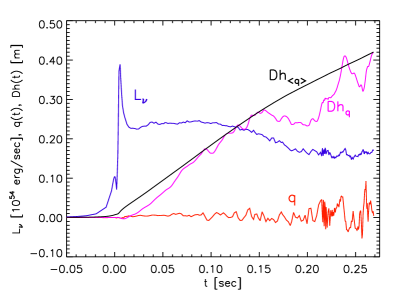
Figure 2: Neutrino luminosity $L_{\nu}(t)$, anisotropy $q(t)$, and GW strain $h(t)$ times distance from anisotropic neutrino emission only, see Eq. (1), for model s15r of Ref. Mueller:2003fs , as functions of time after bounce. We also show the GW strain $h(t)$ times distance from anisotropic neutrino emission, using the average anisotropy $\langle q\rangle=0.45\%$.

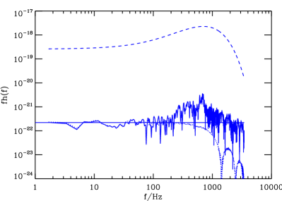
Figure 3: GW source spectra: Solid and dotted ragged lines are total and neutrino contribution, respectively, for model s15r of Ref. Mueller:2003fs at distance $D=10$ kpc. The straight solid line is the low-$f$ tail Eq. (II) with $h_{\infty}$ from Eq. (1), using $q(t)$ and $L_{\nu}(t)$ of Fig. 2, leading to $f|\tilde{h}(f)|\simeq 2.21\times 10^{-22}$. The dashed line is the schematic spectrum for PopIII stars of Eq. (8).

The resulting GW backgrounds are shown in Fig. 4. For model s15r the blue band corresponds to the uncertainty of the enhancement factor discussed above, and the red band is a rough estimate of the uncertainty due to redshift evolution. For $100~{}{\rm Hz}\lesssim f\lesssim 1$ kHz the signal is dominated by the convective motion in the neutrino-heated postshock layer, whereas at lower frequencies it is mostly due to asymmetric neutrino emission. This scenario corresponds to a total energy release in GWs of $\simeq 1.8\times 10^{-8}\,M_{\odot}$ for the most conservative enhancement factor. Note that, although the zero-frequency signal is lower, the GW energy release is higher than in the case of Fig. 1 because it is dominated by high frequencies.

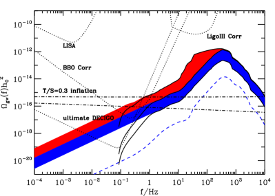
Figure 4: GW background for model s15r with rotation (colored bands and solid lines) and model s11nr180 without rotation (dashed line) from Ref. Mueller:2003fs . The source spectra have been continuously extended using the zero-$f$ tail, Eq. (II), for $f\lesssim 1$ Hz, except for the solid lines. The blue band and lower solid lines for model s15r reflect the plausible range $6$–$36$ of the enhancement factor to correct for the limited time of the simulation. For model s11nr180 the lower enhancement factor of 6 was assumed. We always use $\alpha=0$ in Eq. (7), except for the red band and upper solid line which show the difference between $\alpha=0$ and $\alpha=2$ (for enhancement factor 36) for model s15r.

Equations (II) and (4) show that for our standard redshift evolution ($\alpha=0$ and $\beta=2.7$) and $E_{\nu}\simeq 3\times 10^{53}$ erg liberated in neutrinos, to completely mask the inflation background down to 10 mHz we would need an average anisotropy $\langle q\rangle\simeq 6$%, which is much higher than what is predicted by our most optimistic simulation model s15r where $\langle q\rangle\simeq 0.45\%$. We note that average quadrupole anisotropies $\langle q\rangle$ of the order of 1% are currently not excluded by astrophysical observations. In fact a 1% dipole anisotropy corresponds to observed kick velocities $\simeq 400\,{\rm km}\,{\rm s}^{-1}$ for a neutron star of mass $\simeq 1.4M_{\odot}$, but we do not know whether and how quadrupole and dipole anisotropies are correlated.

For $\alpha\lesssim 2$ in Eq. (7), the integral in Eq. (4) converges rather quickly. Cutting the integral at $z=5$ instead of $z=20$, for example, lowers the predictions by less than a factor 2. In contrast, the poorly constrained redshift evolution for $z>1$ causes more significant uncertainties as illustrated in Fig. 4.

To test the low-frequency dependence on the fluctuations of the neutrino anisotropy, we analyze GW signals for the proto-neutron star model of Ref. Mueller:2003fs whose evolution was followed for 1.2 s. In Fig. 5 we compare the GW spectra for (i) the full simulation integrated over 1.2 s and (ii) the spectrum obtained from replacing the time-dependent anisotropy $q(t)$ of the neutrino emission with its luminosity-weighted average over the 1.2 s duration of the simulation, $\langle q\rangle\sim 3\times 10^{-5}$. The huge difference of $\langle q\rangle$ for models s15r and pns180 arises from the rotation in model s15r, that leads to a global, slowly growing deformation and thus produces a systematic trend on $q(t)$. In contrast, the merely convective fluctuations in model pns180 on time scales of a few milliseconds cause a much lower time-averaged value of $q$.

Figure 5: GW source spectra from mass motions plus anisotropic neutrino emission for the proto-neutron star model pns180 of Ref. Mueller:2003fs at a distance of 10 kpc. The blue curve is for the full simulation with the fluctuating $q(t)$ integrated over 1.2 s, whereas for the red curve $q(t)$ was replaced with $\left\langle q\right\rangle\sim 3\times 10^{-5}$.

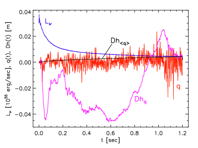
Figure 6: Neutrino luminosity $L_{\nu}(t)$, anisotropy $q(t)$, and GW strain $h(t)$ times distance from anisotropic neutrino emission only, see Eq. (1), for model pns180 of Ref. Mueller:2003fs , as functions of time after bounce. We also show the GW strain $h(t)$ times distance from anisotropic neutrino emission, using the average anisotropy $\langle q\rangle=3\times 10^{-5}$.

From Fig. 5 we conclude the following. For $f\gtrsim 30\,$Hz, replacing $q(t)$ by $\left\langle q\right\rangle$ makes no significant difference (the blue curve is hidden below the red one) because the signal is dominated by convection and thus does not depend on $q(t)$. In contrast, for $1\,{\rm Hz}\lesssim f\lesssim 10\,$Hz, fluctuations in $q(t)$ increase the amplitude by a factor $\simeq 10$. We also note the following technical point due to the properties of Fourier transformations and the SN simulations used here: In the proto-neutron star model pns180 the frequencies covered by the simulation do not extend to the regime where the zero-frequency limit applies, because $L_{\nu}(t)q(t)$ oscillates with an almost constant amplitude over the entire duration of the simulation as seen from Fig. 6, and thus has structure on time scales over which $\exp(i2\pi ft)$ still oscillates even in the lowest frequency bin. If neutrino emission would cease right after the end of the pns180 simulation, $f\tilde{h}(f)$ obtained with the fluctuating $q(t)$, i.e. the blue curve in Fig. 5, should approach $f|\tilde{h}(f)|\to 4\times 10^{-24}$ for $f\ll 1\,$Hz. In contrast, in model s15r the product $L_{\nu}(t)q(t)$ starts out very small over more than half of the simulation time and tends to increase at later times, as seen from Fig. 2. Therefore, in the lowest frequency bin covered by the simulation of model s15r, $\exp(i2\pi ft)$ does not fluctuate significantly over time scales on which $L_{\nu}(t)q(t)$ has structure, and the zero-frequency limit overlaps with the lowest frequencies covered by the simulation.

The GW background for the proto-neutron star models of Fig. 5 is shown in Fig. 7. Due to the redshift effect those GW spectra lie in part in the frequency range of the BBO space-based detectors. Here we are only interested in the relative amplitude between cases (i) and (ii), and not in their absolute amplitude, which is well below the sensitivity of space-based detectors.

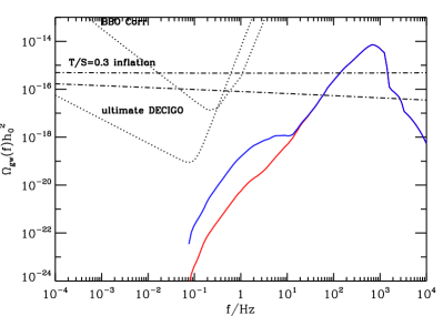
Figure 7: GW background resulting from the source spectrum for the proto-neutron star model pns180 of Ref. Mueller:2003fs shown in Fig. 5 without continuation to $f\lesssim 1\,$Hz. We use $\alpha=0$ in Eq. (7) and an enhancement factor of 3 (about 1/3 of the neutrino energy is emitted until simulation end). The solid blue line thus corresponds to the blue line in Fig. 5 (fluctuating $q(t)$), whereas the solid red line is for $q(t)$ replaced by $\langle q\rangle$ (red line in Fig. 5). Other notation as in Fig. 4.

Finally, the “tail” of the neutrino luminosity during neutrino cooling (times later than 1–2 s after neutron star birth) is known from spherically symmetric neutron star cooling simulations Keil:1995 ; Pons:1998mm ; Thompson:2001ys and can be roughly approximated by $L\propto t^{-n}$ with $n$ around unity (we use $n=1.1$). This in principle could be used to extrapolate the signal to low frequencies. However, the evolution of the anisotropy parameter $q(t)$ during the late phases of proto-neutron star cooling ($\gtrsim\,$1–2 s after bounce) has not been determined by models yet. Any assumption about its behavior after $\sim\,$1 s implies major uncertainties. As discussed above, a constant anisotropy parameter or a fluctuating one can give very different predictions for the GW spectrum in different core-collapse models: For $1\,{\rm Hz}\lesssim f\lesssim 10\,$Hz, the GW source amplitude is suppressed by roughly a factor 10 in model pns180 if $q(t)$ is replaced by a constant equal to its luminosity-weighted average (see Fig. 5). In contrast, for model s15r, the GW source amplitude is almost identical in these two cases in that same frequency range, recall Fig. 3. Similarly, if we evaluate the GW source spectrum by extrapolating the neutrino luminosity decline by $L\propto t^{-1.1}$ and replacing a fluctuating $q(t)$ with a constant equal to its luminosity-weighted average, we would obtain an $h(f)$ smaller by one order of magnitude in the frequency range of space-based detectors. Note that uncertainties in the GW source amplitude of the order of 10 translate into uncertainties in $\Omega_{\rm gw}$ of a factor $\sim 100$.

In conclusion, temporal fluctuations of the neutrino anisotropy are extremely important for predicting the stochastic GW signal at frequencies $f\sim 0.1$ Hz so that longer simulations are needed to make robust predictions.

IV Population III stars

Core collapse events of the hypothetical population III (PopIII) generation of first stars Bromm:2003vv ; Ripamonti:2005ri could be much more efficient emitters of GWs than today’s SN populations Fryer:2000my . Lacking more detailed numerical models, we assume a schematic standard case of a mass of $300\,M_{\odot}$, with a shape of the GW spectrum at $D=10$ kpc resembling that for ordinary SNe shown in Fig. 3,

$$f|\tilde{h}(f)|=2.6\times 10^{-19}\left(1+\frac{f}{0.2~{}{\rm kHz}}\right)^{3}e^{-f/0.3~{}{\rm kHz}}\,.$$ (8)

The normalization implies

$$E_{\rm gw}=\frac{16\pi^{2}D^{2}}{15G_{\rm N}}\,\int df\,|f\tilde{h}(f)|^{2}\simeq 2\times 10^{-3}M_{\odot}$$ (9)

for the total energy emitted in GWs. This very rough estimate is based on hydrodynamical mass motions in 2D geometry Fryer:2000my . If we use the zero-frequency limit of Eq. (II) and $E_{\nu}\simeq 10^{55}$ erg emitted in neutrinos as given in Fig. 9 of Ref. Fryer:2000my for the model with rotation of their Table 1, we find that the average anisotropy would correspond to $\langle q\rangle\simeq 3\%$ in this case. While this is significantly larger than the values expected for ordinary SNe, it may not be unrealistic, given that PopIII stars tend to rotate more rapidly and explode more violently.

Finally, we assume that the PopIII rate is concentrated around a redshift $z_{\rm III}=15$, which may explain reionization Kogut:2003et . We thus write for the PopIII rate $R_{\rm SN}(z)=R\delta(z-z_{\rm III})$, where $R$ is a normalization constant. We further assume that all PopIII stars have a progenitor mass $M_{\rm III}=300M_{\odot}$. The total number of PopIII events per comoving volume that occurred up to $z=0$ can then be written as

$$\int_{0}^{\infty}dtR_{\rm SN}(z)=\frac{R}{(1+z_{\rm III})H(z_{\rm III})}=f_{\rm III}\,n_{\gamma}\,\eta\,\frac{m_{N}}{M_{\rm III}}\,,$$ (10)

where $n_{\gamma}\simeq 410\,{\rm cm}^{-3}$ is the CMBR photon density at redshift zero, $\eta\simeq 6.3\times 10^{-10}$ is the number of baryons per CMBR photon, $m_{N}$ is the nucleon mass, and $f_{\rm III}$ is the fraction of all baryons going through PopIII stars. Eliminating $R$, it then follows that the rate observed at Earth, $R_{\rm III}$ given in Eq. (6), is directly proportional to $f_{\rm III}$,

$$R_{\rm III}\simeq 4\pi r^{2}(z_{\rm III})\,f_{\rm III}n_{\gamma}\eta\,\frac{m_{N}}{M_{\rm III}}\,.$$ (11)

For the parameters given above this yields $R_{\rm III}\simeq 0.2\,(f_{\rm III}/10^{-3})\,{\rm s}^{-1}$.

The resulting GW background is shown in Fig. 8 as a band delimited by two extreme assumptions about the total cosmic PopIII core-collapse rate observed from Earth, i.e. $R_{\rm III}\simeq 0.2~{}{\rm s}^{-1}$  (upper edge of band) and $\simeq 4.4\times 10^{-4}~{}{\rm s}^{-1}$ Wise:2004zp (lower edge). The zero-frequency limit would affect the GW spectrum only at frequencies below 0.05 Hz. We remark that certain models attempting to explain the near infrared excess with PopIII stars require baryon fractions as high as $f_{\rm III}\simeq 0.05$ Madau:2005wv , corresponding to rates $R_{\rm III}\simeq 10\,{\rm s}^{-1}$ and GW backgrounds a factor $\sim 50$ still higher than the upper band shown in Fig. 8. Rates corresponding to $R_{\rm III}\simeq 1\,{\rm s}^{-1}$ are discussed in Ref. Mesinger:2005du . The problem with such high-rate scenarios is to avoid overproduction of metals.

Whereas neutrinos from PopIII stars are redshifted to energies probably too low to be detected Iocco:2004wd , the GW background for $10~{}{\rm mHz}\lesssim f\lesssim 1~{}{\rm kHz}$ could be dominated by these objects.

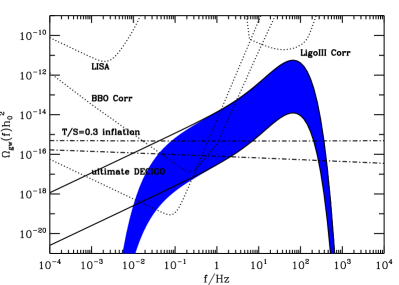
Figure 8: GW background for our standard PopIII core collapse case and event rates $4.4\times 10^{-4}~{}{\rm s}^{-1}<R_{\rm III}<0.2~{}{\rm s}^{-1}$. For the blue shaded band the source spectrum shown in Fig. 3 was cut off at $f\leq 1\,$Hz and in this sense does not rely on the zero-frequency limit. The solid lines are obtained from continuing the source signal by the zero-frequency limit.

V Gaussianity

Finally, we estimate the duty cycle of the background at a given frequency $f$. It is defined as the product of the rate of events and the time scale of interest, $f^{-1}$.

The duty cycle is roughly given by dividing the total cosmic SN rate, Eq. (6), by the frequency. A probably more realistic estimate is obtained by folding the rate integral over redshift with the redshift dependent contribution to the GW signal given by the integrand in Eq. (4). For model s15r of Ref. Mueller:2003fs and the evolution discussed around Eq. (7) these two estimates give approximately $33\,(f/{\rm Hz})^{-1}$ and $4\,(f/{\rm Hz})^{-1}$, respectively.

The signal from ordinary SNe becomes Gaussian for $f\lesssim 1$ Hz, in agreement with a cosmic SN rate of about $1~{}{\rm s}^{-1}$. In contrast, the backgrounds in the $10^{2}\mbox{--}10^{3}$ Hz range are not Gaussian, consistent with Ref. Schneider:1999us where only the bounce signal was considered that lasts about $10^{-3}$ s. At these frequencies the duty factor is $\lesssim 1\%$. The putative PopIII background becomes Gaussian only for $f\lesssim R_{\rm III}$, i.e. probably for $f\lesssim 0.1$ Hz.

VI Conclusions

The GW background from cosmological core-collapse SNe at frequencies below 1 Hz is Gaussian. Its power is uncertain by several orders of magnitude, mostly due to uncertainties of SNe as GW sources. The most important uncertain parameters are the asymmetry parameter $\langle q\rangle$ of late-time neutrino emission and the parameter $\alpha$ determining the star-formation rate at redshifts $z>1$ [see Eq. (7)]. The most optimistic current simulations (for stellar core collapse with rotation) predict $\langle q\rangle\sim 0.45\%$, whereas Super-K limits on the diffuse neutrino background constrain $\alpha$ in the range $0\lesssim\alpha\lesssim 2$. Using these parameter values and extrapolating the GW signal with the zero-frequency limit, Eq. (II), to the frequency band of space-based detectors, we showed that the GW background from SNe could be comparable to the maximum signal expected from standard inflationary models and thus could be detected by second-generation space-based detectors. However, to completely mask the inflationary background down to 10 mHz, we would need a very large asymmetry of $\langle q\rangle\sim 6\%$, that is not compatible with current simulations. By using the proto-neutron star model of Ref. Mueller:2003fs , for which the simulation continues until 1.2 s, we observed that the GW spectra at frequencies of interest for future space-based detectors depends strongly on the fluctuations of $q(t)$. Predictions could differ by a few orders of magnitude if $q(t)$ continues to fluctuate for all or part of the neutrino cooling phase even after 1 s of neutron star cooling.

Numerical simulations and stronger constraints or detections of the corresponding neutrino background will lead to an improved prediction of the GW background. However, accurate calculations of the GW emission from core collapse are hampered by our incomplete knowledge of important input physics like the equation of state at nuclear and supernuclear densities, of initial conditions like the structure of stellar cores at the onset of gravitational collapse, and the amount of rotation and size of magnetic fields in the pre-collapse core. More reliable GW predictions also require a better understanding of the explosion mechanism and improvements in the numerical modeling of SNe. Quantitatively meaningful calculations will have to be done in 3D, will have to include a decent treatment of general relativistic effects, and will have to be done with full 3D neutrino transport in order to determine the neutrino emission anisotropy on all angular scales and at all frequencies. Three-dimensional effects are expected to reduce the emission anisotropy of neutrinos because of smaller convective structures mueller2 and because of the tendency of multi-dimensional transport to reduce the power on high spatial frequencies. In contrast, significant rotation and large-scale magnetic fields might cause global emission anisotropies with possibly constant anisotropy parameter and high power at low frequencies. It is left to future generations of SN models to shed light on these important questions.

PopIII stars could give a particularly strong contribution, masking almost completely the inflationary background, if we use the upper range Daigne:2004ga of the very uncertain rate predictions Wise:2004zp ; Madau:2005wv ; Mesinger:2005du in the literature and assume a total energy emitted in GWs of $2\times 10^{-3}M_{\odot}$. For typical event rates and/or lower values of the total GW energy emitted, the GW spectrum from PopIII stars could be comparable to or lower than the one expected from inflation. In this case the zero-frequency limit would influence the GW spectrum only at frequencies below 0.05 Hz. In any event, the largest problem for a reliable prediction of the GW background from stellar core collapse is the almost complete lack of theoretical understanding of massive PopIII stars as GW sources and the extreme uncertainty of their abundance, in fact the uncertainty of their very existence.

In summary, the uncertainties of the stochastic GW background from the core collapse of ordinary SNe and from PopIII stars is large, but it is intriguing that its power is in the ball park of the maximum GW background expected from inflationary models. Of course, the inflationary GW background itself is also very uncertain and could be smaller than the benchmark shown in our figures. If stochastic GWs are detected with a future instrument like the BBO, it may be challenging to disentangle the inflationary GWs from those caused by SNe or the collapse of PopIII stars.

- (1) M. Malek et al. [Super-Kamiokande Collab.], “Search for supernova relic neutrinos at Super-Kamiokande,” Phys. Rev. Lett. 90, 061101 (2003) [hep-ex/0209028].
- (2) L. E. Strigari, M. Kaplinghat, G. Steigman and T. P. Walker, “The supernova relic neutrino backgrounds at KamLAND and Super-Kamiokande,” JCAP 0403, 007 (2004) [astro-ph/0312346]
- (3) S. Ando and K. Sato, “Relic neutrino background from cosmological supernovae,” New J. Phys. 6, 170 (2004) [astro-ph/0410061].
- (4) L. E. Strigari, J. F. Beacom, T. P. Walker and P. Zhang, “The concordance cosmic star formation rate: Implications from and for the supernova neutrino and gamma ray backgrounds,” JCAP 0504, 017 (2005) [astro-ph/ 0502150].
- (5) J. F. Beacom and M. R. Vagins, “Antineutrino spectroscopy with large water Čerenkov detectors,” Phys. Rev. Lett. 93, 171101 (2004) [hep-ph/0309300].
- (6) E. Müller, M. Rampp, R. Buras, H.-T. Janka and D. H. Shoemaker, “Towards gravitational wave signals from realistic core collapse supernova models,” Astrophys. J. 603, 221 (2004) [astro-ph/0309833].
- (7) C. L. Fryer, D. E. Holz and S. A. Hughes, “Gravitational waves from stellar collapse: Correlations to explosion asymmetries,” Astrophys. J. 609, 288 (2004) [astro-ph/0403188].
- (8) R. Epstein, “The generation of gravitational radiation by escaping supernova neutrinos,” Astrophys. J. 223, 1037 (1978).
- (9) E. Müller and H.-T. Janka, “Gravitational radiation from convective instabilities in Type II supernova explosions,” Astron. Astrophys. 317, 140 (1997).
- (10) M. S. Turner, “Gravitational radiation from supernova neutrino bursts,” Nature 274, 565 (1978).
- (11) L. Smarr, “Gravitational radiation from distant encounters and from headon collisions of black holes: The zero frequency limit,” Phys. Rev. D 15, 2069 (1977).
- (12) V. B. Braginsky and K. T. Thorne, “Gravitational-wave bursts with memory and experimental prospects,” Nature 327, 123 (1987).
- (13) A. Burrows and J. Hayes, “Pulsar recoil and gravitational radiation due to asymmetrical stellar collapse and explosion,” Phys. Rev. Lett. 76, 352 (1996) [astro-ph/9511106].
- (14) R. J. Bontz and R. H. Price, “The spectrum of radiation at low frequencies,” Astrophys. J. 228, 560 (1979).
- (15) F. Daigne, K. A. Olive, E. Vangioni-Flam, J. Silk and J. Audouze, “Cosmic star formation, reionization, and constraints on global chemical evolution,” strophys. J. 617, 693 (2004) [astro-ph/0405355].
- (16) E. S. Phinney, “A practical theorem on gravitational wave backgrounds,” [astro-ph/0108028].
- (17) M. S. Turner, “Detectability of inflation-produced gravitational waves,” Phys. Rev. D 55, R435 (1997) [astro-ph/960706].
- (18) E. S. Phinney, private communication.
- (19) R. Buras, M. Rampp, H.-T. Janka and K. Kifonidis, “Improved models of stellar core collapse and still no explosions: What is missing?,” Phys. Rev. Lett. 90, 241101 (2003) [astro-ph/0303171].
- (20) H.-T. Janka, R. Buras, K. Kifonidis and M. Rampp, “Core-collapse supernovae at the threshold,” in: Cosmic Explosions, eds. J. M. Marcaide and K. W. Weiler (Springer, Berlin, 2005) p. 253 [astro-ph/0401461].
- (21) R. Buras, M. Rampp, H.-T. Janka and K. Kifonidis, “Two-dimensional hydrodynamic core-collapse supernova simulations with spectral neutrino transport. I. Numerical method and results for a star,” astro-ph/0507135.
- (22) W. Keil, H.-T. Janka and E. Müller, “Ledoux-convection in protoneutron stars: A clue to supernova nucleosynthesis?,” Astrophys. J. 473, L111 [astro-ph/9610203].
- (23) W. Keil, “Konvektive Instabilitäten in entstehenden Neutronensternen,” PhD Thesis, TU München (unpublished).
- (24) H. T. Janka and W. Keil, “Perspectives of core-collapse supernovae beyond SN1987A,” in: Supernovae and Cosmology, ed. L. Labhardt, B. Binggeli, and R. Buser (Astronomisches Institut Univ. Basel, Basel, 1998), p. 7 [astro-ph/9709012].
- (25) H.-T. Janka, K. Kifonidis and M. Rampp, “Supernova explosions and neutron star formation,” in: Physics of Neutron Star Interiors, Lect. Notes Phys. 578, 333 (2001) [astro-ph/0103015].
- (26) R. Walder, A. Burrows, C.D. Ott, E. Livne, I. Lichtenstadt and M. Jarrah, “Anisotropies in the neutrino fluxes and heating profiles in two-dimensional, time-dependent, multi-group radiation hydrodynamics simulations of rotating core-collapse supernovae,” Astrophys. J. 626, 317 (2005) [astro-ph/0412187].
- (27) A. Buonanno, “TASI Lectures on Gravitational waves from the early universe,” gr-qc/0303085.
- (28) N. Seto, S. Kawamura and T. Nakamura, “Possibility of direct measurement of the acceleration of the universe using 0.1-Hz band laser interferometer gravitational wave antenna in space,” Phys. Rev. Lett. 87, 221103 (2001) [astro-ph/0108011].
- (29) W. Keil and H.-T. Janka, “Hadronic phase transitions at supranuclear densities and the delayed collapse of newly formed neutron stars,” Astron. Astrophys. 296, 145 (1995).
- (30) J. A. Pons, S. Reddy, M. Prakash, J. M. Lattimer and J. A. Miralles, “Evolution of protoneutron stars,” Astrophys. J. 513, 780 (1999) [astro-ph/9807040].
- (31) T. A. Thompson, A. Burrows and B. S. Meyer, “The physics of protoneutron star winds: Implications for r-process nucleosynthesis,” Astrophys. J. 562, 887 (2001) [astro-ph/0105004].
- (32) V. Bromm and R. B. Larson, “The first stars,” Ann. Rev. Astron. Astrophys. 42, 79 (2004) [astro-ph/0311019].
- (33) E. Ripamonti and T. Abel, “The formation of primordial luminous objects,” astro-ph/0507130.
- (34) C. L. Fryer, S. E. Woosley and A. Heger, “Pair-instability supernovae, gravity waves, and gamma-ray transients,” Astrophys. J. 550, 372 (2001) [astro-ph/0007176].
- (35) A. Kogut et al., “Wilkinson Microwave Anisotropy Probe (WMAP) first year observations: TE polarization,” Astrophys. J. Suppl. 148, 161 (2003) [astro-ph/0302213].
- (36) J. H. Wise and T. Abel, “The number of supernovae from primordial stars in the universe,” astro-ph/0411558.
- (37) P. Madau and J. Silk, “Population III and the near-infrared backround excess,” astro-ph/0502304.
- (38) A. Mesinger, B. Johnson and Z. Haiman, “Probing reionization with the redshift distribution of distant supernovae,” astro-ph/0505110.
- (39) F. Iocco, G. Mangano, G. Miele, G. G. Raffelt and P. D. Serpico, “Diffuse cosmic neutrino background from population III stars,” Astropart. Phys. 23, 303 (2005) [astro-ph/0411545].
- (40) R. Schneider, A. Ferrara, B. Ciardi, V. Ferrari and S. Matarrese, “Gravitational wave signals from the collapse of the first stars,” Mon. Not. Roy. Astron. Soc. 317, 385 (2000) [astro-ph/9909419].