Performance analysis of direct $N$-body algorithms for astrophysical simulations on distributed systems

Abstract

We discuss the performance of direct summation codes used in the simulation of astrophysical stellar systems on highly distributed architectures. These codes compute the gravitational interaction among stars in an exact way and have an $O(N^{2})$ scaling with the number of particles. They can be applied to a variety of astrophysical problems, like the evolution of star clusters, the dynamics of black holes, the formation of planetary systems, and cosmological simulations. The simulation of realistic star clusters with sufficiently high accuracy cannot be performed on a single workstation but may be possible on parallel computers or grids. We have implemented two parallel schemes for a direct $N$-body code and we study their performance on general purpose parallel computers and large computational grids. We present the results of timing analyzes conducted on the different architectures and compare them with the predictions from theoretical models. We conclude that the simulation of star clusters with up to a million particles will be possible on large distributed computers in the next decade. Simulating entire galaxies however will in addition require new hybrid methods to speedup the calculation.

, and

1 Introduction

Numerical methods for solving the classical astrophysical $N$-body problem have evolved in two main directions in recent years. On the one hand, approximated models like Fokker-Planck models [1], [2], gaseous models [3], and Monte Carlo models [4], [5], [6] have been applied to the simulation of globular clusters and galactic nuclei. These models permit to follow the global evolution of large systems along their lifetime but at the expense of moderate accuracy and resolution. The basic approach is to group particles according to their spatial distribution and use a truncated multipole expansion to evaluate the force exerted by the whole group instead of evaluating directly the contributions from the single particles. On the other hand, direct summation methods have been developed to accurately model the dynamics and evolution of collisional systems like dense star clusters. These codes compute all the inter-particle forces and are therefore the most accurate. They are also more general, as they can be used to simulate both low and high density regions. Their high accuracy is necessary when studying physical phenomena like mass segregation, core collapse, dynamical encounters, formation of binaries or higher order systems, ejection of high velocity stars, and runaway collisions. Direct methods have an $O(N^{2})$ scaling with the number of stars and are therefore limited to smaller particle numbers compared to approximated methods. For this reason, so far they have only been applied to the simulation of moderate size star clusters. The simulation of globular clusters containing one million stars is still a challenge from the computational point of view, but it is an important astrophysical problem. It will provide insight in the complex dynamics of these collisional systems, in the microscopic and macroscopic physical phenomena, and it will help finding evidence of the controversial presence of a central black hole. The simulation of the evolution of these systems under the combined effects of gravity, stellar evolution, and hopefully hydrodynamics will allow to study the stellar population and to compare the results with observations.

The need to simulate ever larger systems and to include a realistic physical treatment of stars asks for a speedup in the most demanding part of the calculation: the gravitational dynamics. Significant improvement in the performance of direct codes can be obtained either by means of special purpose computers like GRAPE hardware [7] or of general purpose distributed systems [8]. In this work, we focus on the performance of direct $N$-body codes on distributed systems. Two main classes of algorithms can be used to parallelize direct summation $N$-body codes: replicated data and distributed data algorithms. In this work we present a performance analysis of the two algorithms on different architectures: a Beowulf cluster, three supercomputers, and two computational grids. We provide theoretical predictions and actual measurements for the execution time on different platforms, allowing the choice of the best performing scheme for a given architecture.

2 Numerical method

In the direct method the gravitational force acting on a particle is computed by summing up the contributions from all the other particles according to Newton’s law

$$\mathbf{F}_{i}=m_{i}\mathbf{a}_{i}=-Gm_{i}\sum_{j=1,j\neq i}^{j=N}\frac{m_{j}(\mathbf{r}_{i}-\mathbf{r}_{j})}{|\mathbf{r}_{i}-\mathbf{r}_{j}|^{3}}.$$ (1)

The number of force calculations per particle is $N(N-1)/2$ . Given the fact that the force acting on a particle usually varies smoothly with time, the integration of the particle trajectory makes use of force polynomial fitting. In this work we implement the fourth-order Hermite integrator with a predictor-corrector scheme and a hierarchical time-step.

In the Hermite scheme [9] high order derivatives are explicitly computed to construct interpolation polynomials of the force. After the group of particles to be integrated at time $t$ has been selected, the positions and velocities of all particles are predicted at time $t$ (predictor phase) using the values of positions, velocities, accelerations, and first derivative of accelerations (hereafter jerks) computed at the previous step. The prediction uses a third order Taylor expansion. By means of the predicted quantities, new values of the accelerations and jerks at time $t$ are computed. This calculation is the most computationally expensive of the whole scheme, having a $N^{2}$ scaling. The second and third derivative of the accelerations are then calculated using the Hermite interpolation based on the values of acceleration and jerk. These correcting factors are added to the predicted positions and velocities (corrector phase) at time $t$. The new time-step of the particles is estimated according to the time-step prescription in use and the time of the particles is updated.

The hierarchical time-step scheme is a modification of the individual time-step scheme in which groups of particles are forced to share the same time-step. In the individual time-step scheme every particle has its own time $t_{i}$ and its own time-step $\Delta t_{i}$, with a step-size depending on the value of the acceleration $a_{i}$ and its higher order derivatives $a_{i}^{(n)}$ according to

$$\Delta t_{i}=\sqrt{\eta\frac{|\mathbf{a}_{i}||\mathbf{a}_{i}^{(2)}|+|\mathbf{a}_{i}^{(1)}|^{2}}{|\mathbf{a}_{i}^{(1)}||\mathbf{a}_{i}^{(3)}|+|\mathbf{a}_{i}^{(2)}|^{2}}},$$ (2)

where $\eta$=0.01 is a dimensionless accuracy parameter. Only particles requiring a short time-step are integrated with such a short step-size, while other particles can be integrated with a longer one. This reduces the total calculation cost by a factor $O(N^{1/3})$ with respect to a shared time-step code, where all the particles share the same time-step [10]. However, it is not efficient to use the individual time-step scheme in its original form on a parallel computer since only one particle is integrated at each step, that is the particle with the smallest value of $t_{i}+\Delta t_{i}$. In order to fully exploit a parallel code, several particles need to be updated at the same time, or, equivalently, several particles need to share the same time-step. In the hierarchical or block time-step scheme [11] the time-steps are quantized to powers of two, so that a group of particles can be advanced at the same time. After the computation of $\Delta t_{i}$ according to the individual time-step prescription, the largest power of two smaller than $\Delta t_{i}$ is actually assigned as a time-step to the particle under consideration. The group of particles sharing the same time-step are said to form a block. The use of block time-steps results in a better performance since it permits to advance several particles simultaneously: the computation of the force exerted upon the particles in a block and the integration of the trajectories can be done in parallel by different processors. Furthermore, the positions and velocities in the predictor phase need to be calculated only once for these particles.

3 Parallel schemes for direct $N$-body codes

The parallelization of a direct $N$-body code can proceed in different ways depending on the desired intrinsic degree of parallelism and communication to computation ratio. We implemented two different parallelization algorithms, the copy algorithm and the ring algorithm, for an Hermite scheme with block time-steps using the standard MPI library package. If we denote with $N$ the total number of particles in the system and with $p$ the number of available processors, both algorithms have a theoretical computational complexity $O(Np)$ for the communication and $O(N^{2}/p)$ for the calculation (see $\S$ 4 for a derivation of more detailed scaling relations).

3.1 The copy algorithm

The copy algorithm [12], also called the “replicated data algorithm” [8], is a parallelization scheme which relies on the assumption that each processor has a local copy of the whole system. A schematic representation of the copy algorithm is shown in Fig. 1.

Figure 1: Schematic representation of the force calculation in the copy algorithm in the simple case of $p$=4 processors and $N$=24 particles. Each processor has a local copy of the whole system but at step 1 is also assigned $n$=6 particles (selected particles). Among these, at step 2 each processor selects the local subgroup $s_{i}$ of the block of particles to be updated (circled particles). At step 3 each node calculates the total force exerted by all the $N$ particles (those on top of the arrow) on the selected particles (those below the arrow). At step 4 every processor broadcasts the new data to all the other processors. For clarity only the communication operations (indicated with arrows) of processor 0 and 1 are shown in the figure.

At each integration step, the particles to be advanced are distributed among the processors. The nodes proceed in parallel to the computation of the forces exerted by all the $N$ particles on the local particles, of the trajectories, and of the new time-steps. At the end of the step all the processors broadcast the new data to all the other processors for a complete update.

This algorithm minimizes the amount of communication since it only requires one collective communication at the end of each step. The main disadvantage is its limitation in memory because of the need to store the data relative to all the particles on each node. This scheme may suffer from load imbalance as the number of particles to update can be different for the different nodes. For high numbers of particles, however, a random initial distribution is sufficient to ensure a relatively good balance.

3.2 The ring algorithm

The ring or systolic algorithm makes use of a virtual ring topology of the processors to circulate the particles which need to be advanced. In this scheme, each processor is assigned a group of $n=N/p$ particles and only needs to store the data relative to those particles throughout the whole integration. Therefore, the scheme has the advantage of minimizing the memory requirements on each node. A schematic representation of the ring algorithm is shown in Fig. 2.

Figure 2: Schematic representation of the force calculation in the ring algorithm in the simple case of $p$=4 processors and $N$=24 particles. The processors are virtually connected in a ring-like structure topology. At the beginning every processor has $n$=6 particles and a subset $s_{i}$ of them needs to be updated. Each node starts computing the partial forces exerted by its $n$ particles on those in the block. At step 1 each processor sends the data relative to the $s_{i}$ particles (circled particles in the first row) to its right neighbor, receives particles (second row) from the left neighbor and computes the force on the received particles (those below the arrow). The force computation is indicated with vertical arrows. The same procedure is repeated in step 2 and 3 until in step 4 the total forces on the block of particles are computed and the $s_{i}$ particles are returned to their owners.

Among all the particles that need to be updated, each processor selects those belonging to its local group. The initialization, the predictor phase and the corrector phase are performed in parallel by all the processors on their local subgroup of particles. When the acceleration on the subgroup needs to be computed, each node first calculates the partial forces exerted by all the $n$ particles and then sends the data (including the partial acceleration) to the processor which is defined as the right neighbor in the virtual topology. At the same time, the node receives data from its left neighbor and starts incrementing the accelerations exerted by its local $n$ particles on the received ones. After $p$ shifts, the complete forces are calculated and the particles are returned to their original processors for the computation of the trajectory and the update of the time and time-step values.

The ring algorithm can be implemented using MPI non-blocking communication routines [8]. This technique is called latency hiding and is most efficient in the case of small number of particles or of very concentrated models, when the block sizes are smaller and hence the load imbalance becomes more important. Non-blocking MPI communication routines allow the separation between the initiation and the completion of a communication by returning immediately after the start of the communication. In this way, some computation can be performed at the same time as the sending and receiving of data is ongoing. The implementation of non-blocking communication in our Hermite code exploits the property that the computation of the force only requires the positions and velocities of the particles. The transfer of positions and velocities can then be separated from the transfer of accelerations and jerks. In each shift of the systolic scheme, the communication is split in two branches and overlaps with the computation of new forces and their derivatives. The branch of accelerations and jerks follows one step behind that of positions and velocities. As a consequence of that, the transfer of the forces starts only at the second shift and one final transfer is necessary at the end of the last shift.

4 Performance analysis of different parallel $N$-body schemes

The performance of a parallel code does not only depend on the properties of the code itself, like the parallelization scheme and the intrinsic degree of parallelism, but also on the properties of the parallel computer used for the computation. The main factors determining the general performance are the calculation speed of each node, the bandwidth of the inter-processor communication, and the start-up time (latency). A theoretical estimate of the total time needed for one full force calculation loop must take into account the properties of the parallel computer [8], [12]. Table 1 shows the hardware specifications of the different platforms used for our performance runs: a Beowulf cluster, a SGI Origin supercomputer (Teras), an experimental low latency cluster (DAS-AMS), and a state-of-the-art computer cluster (Lisa).

Table 1: Specifications for the different distributed architectures.

	Beowulf	Teras	DAS-AMS	Lisa
OS	Linux	Irix	Linux	Linux
Compiler	gcc-2.95.4	gcc-3.0.4	gcc-2.96	gcc-3.3
CPU	AMD Athlon	MIPS R14000	Pentium-III	Intel Xeon
CPU speed	700 MHz	500 MHz	1 GHz	3.4 GHz
Network	Fast Ethernet	Gbit Ethernet	Myrinet-2000	Infiniband
$\tau_{f}$ [sec]	5.5$\times 10^{-7}$	3.5$\times 10^{-7}$	4.5$\times 10^{-7}$	1.2$\times 10^{-7}$
$\tau_{l}$ [sec]	5.0$\times 10^{-5}$	2.0$\times 10^{-5}$	1.0$\times 10^{-5}$	5.0$\times 10^{-6}$
$\tau_{c}$ [sec]	8.0$\times 10^{-4}$	1.5$\times 10^{-4}$	1.5$\times 10^{-4}$	5.0$\times 10^{-5}$

The Beowulf cluster and Teras are hosted by the SARA computing and networking services center in Amsterdam. DAS-2 is a wide-area distributed computer composed by clusters located at five different universities in the Netherlands. For the tests described in this section we only use the nodes in Amsterdam (DAS-AMS) which are interconnected by a fast and low latency network. Lisa is the Dutch national computer cluster hosted by SARA. In the Table we report the specifications, the time $\tau_{f}$ for the computation of one inter-particle force, the time $\tau_{l}$ for the start-up of a communication, and the time $\tau_{c}$ needed to send the data relative to one particle to another processor. The parameters represent the fits to the data presented in $\S$4.1 and $\S$4.2.

To measure the performance of our code and to compare the results with the theoretical estimates, we consider the total wall-clock time for an integration of one $N$-body time-unit [13]. Our code employs “standard N-body units” [13], according to which the gravitational constant, the total mass, and the radius of the system are taken to be unity. The resulting unit for time is called $N$-body time-unit and is related to the physical crossing time of the system through the relation $T_{\rm cross}=2\sqrt{2}$. This time is proportional to the number of particles in the system and represents therefore a suitable unit to check the dependency of the execution time on $N$.

4.1 Performance of the copy algorithm

The time needed for the computation of the force on a block of particles of certain size can be estimated as follows. Let $s$ be the number of particles to be updated at a particular step (block size) and let $s_{i}$ be the size of the subgroup of particles that processor of rank $i$ has to update so that $s=\sum_{i=1}^{p}s_{i}$. The values of $s_{i}$ will in general be different and the total time for the computation will be determined by the processor with the largest block size $s_{\rm max}=\max_{i=1,\dots p}\left\{s_{i}\right\}\thinspace.$ If we indicate with $\tau_{f}$ the time needed for one computation of the force between two particles, then the time to compute the force on the block of particles is given by $T_{\rm calc}=\tau_{f}Ns_{\rm max}$, since all the processors need to wait until the one with the largest block of particles has terminated. The time for the communication taking place at the end of the computation is given by $T_{\rm comm}=\tau_{l}p+\sum_{i=1}^{p}\tau_{c}s_{i}=\tau_{l}p+\tau_{c}s$, where $\tau_{l}$ is the latency and $\tau_{c}$ is the time needed to send the data relative to one particle from one processor to another. The total time to compute the force on the block of $s$ particles is

$$T_{\rm force}=T_{\rm calc}+T_{\rm comm}=\tau_{f}Ns_{\rm max}+\tau_{l}p+\tau_{c}s\thinspace.$$ (3)

Eq. (3) shows how the time for the force computation depends on the speed of calculation of each processor, on the latency, and on the bandwidth of communication. If we rewrite $s_{\rm max}=s/p+\delta$, where the parameter $\delta$ represents the deviation from the mean value ($\delta\propto\sqrt{s/p}$), then the calculation time scales as $T_{\rm calc}\propto 1/p$ while the communication time scales as $T_{\rm comm}\propto p$.

In Fig. 3 we report the total wall-clock time for an integration of a Plummer model [14] with equal mass stars in virial equilibrium for one $N$-body time-unit using the copy algorithm on the four different architectures (Table 1)

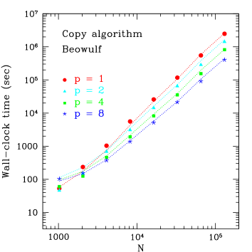
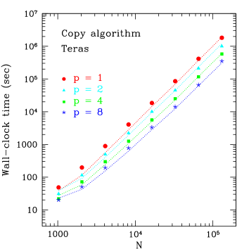
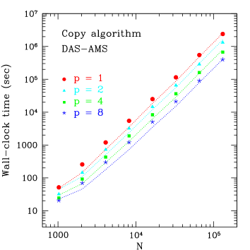
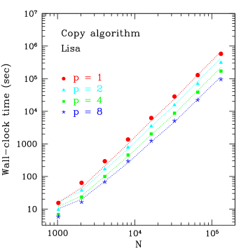
Figure 3: Wall-clock time as a function of the number of particles for the copy algorithm on the four different architectures. The symbols represent the data obtained from the timing measurements while the dotted lines represent the predictions by the performance model.

The symbols represent the data obtained from the timing measurements while the dotted lines represent the predictions by the theoretical model. Given the long execution times for large $N$, the measurements shown in the plot were performed only once. Nonetheless, we performed more measurements for a few cases to assess the typical uncertainties associated with the timings and we found that the errors are always smaller than 10%. For large $N$, when the system is calculation dominated, the performance is similar on the Beowulf, Teras and DAS-AMS computers, while it is significantly better for the Lisa cluster. For small $N$, when the system is communication dominated, the execution times are shorter on the clusters with faster network, and this is especially true for a larger number of processors. For a fixed number of particles, the parallelization efficiency of the copy algorithm reduces as the number of processors increases. This is due to the ever increasing amount of communication which takes place as the number of processors becomes larger. On the other hand, for a fixed processor number, the efficiency increases as the number of particles increases. For larger $N$, in fact, the block sizes become larger and the particles in the block tend to be more evenly distributed among the available nodes (i.e. $\delta\rightarrow 0$). Load imbalance can affect the performance of any parallel code and is a result of the use of block time-steps. Fortunately, for a large number of particles a good load balance is achieved if the particles are randomly assigned to the processors in the initialization phase. The theoretical model used to predict the execution time is based on Eq. (3) with the parameters reported in Table 1. Since the block size is different at each integration step, the total time for one $N$-body time-unit is obtained considering the measured average block size $\langle s\rangle\sim 0.1\,N^{2/3}$. The agreement between the model and the measured times is generally good and improves for large $N$, which is the regime of interest for $N$-body simulations.

4.2 Performance of the ring algorithm

In the case of the ring algorithm with blocking communication the total time for one full force loop calculation can be estimated as follows. If we first consider the time for one shift in the ring, the time to compute the force on the local subgroups of particles $s_{i}$ is given by $T_{\rm calc,1shift}=\tau_{f}ns_{\rm max}$, while the time for communication is given by $T_{\rm comm,1shift}=\tau_{l}+\tau_{c}s_{\rm max}$. After $p$ shifts in the ring, the total time to compute the force on the block of $s$ particles is

$$T_{\rm force}=\left(T_{\rm calc,1shift}+T_{\rm comm,1shift}\right)p=\tau_{f}Ns_{\rm max}+\tau_{l}p+\tau_{c}ps_{\rm max}$$ (4)

where we have substituted $n=N/p$. As in the case of the copy algorithm, the time for the force computation depends on the speed of calculation of each processor, on the latency, and on the bandwidth of communication. A comparison of Eq. (3) and Eq. (4) shows how the computation time required by the two algorithms is exactly the same while the communication time is generally slightly shorter for the copy algorithm. In the special case $s_{\rm max}=s/p$, the communication time for the ring algorithm equals that of the copy algorithm.

If the block size is the same for all the processors, for example $s_{i}=s/p$, the total time for the force calculation is given by

$$T_{\rm force}=\tau_{f}N\frac{s}{p}+\tau_{l}p+\tau_{c}s\thinspace.$$ (5)

The value $p_{\rm eq}$ of the number of processors for which the calculation time and the communication time are equal is given by

$$p_{\rm eq}=\frac{-\tau_{c}s+\sqrt{\tau_{c}^{2}s^{2}+4\tau_{l}\tau_{f}Ns}}{2\tau_{l}}\thinspace.$$ (6)

Since the calculation time monotonically decreases as a function of $p$ while the communication time monotonically increases as a function of $p$, there exists a specific value $p_{\rm min}$ for the number of processors which minimizes the total time. Solving for the minimum yields $p_{\rm min}=\sqrt{\frac{\tau_{f}}{\tau_{l}}Ns}\thinspace$. For moderately concentrated models, $s\propto N^{2/3}$ [15] and hence $p_{\rm min}\propto N^{5/6}$. In the simple case $s_{i}=s/p$, the time to compute the force exerted on the block of particles is the same for the copy and the ring algorithms, and therefore the expressions for $p_{\rm eq}$ and $p_{\rm min}$ hold for both schemes. In the more general case of different $s_{i}$, the expressions for $p_{\rm eq}$ and $p_{\rm min}$ differ slightly.

In the case of a shared time-step code the block size is the same for all the processors and is given by $s_{i}=n$. The total time for the force calculation becomes

$$T_{\rm force}=\tau_{f}\frac{N^{2}}{p}+\tau_{l}p+\tau_{c}N$$ (7)

so that for a fixed number of particles $T_{\rm calc}\propto 1/p$ and $T_{\rm comm}\propto p$. Fig. 4 shows the calculation and communication time as a function of the number of processors for a fixed number of particles.

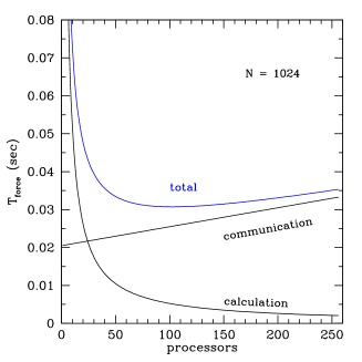
Figure 4: Theoretical estimate of the total time for one full force loop obtained from Eq. (5) in the simple case $N=1024$, $s_{i}=N/p$ for each processor, using the parameters for a Beowulf cluster (see Table 1). The calculation time scales as $T_{\rm calc}\propto 1/p$ while the communication time scales as $T_{\rm comm}\propto p$ so that there exists a particular value of the processor number for which the two times are equal. In this case $p_{\rm eq}=24$. The number of processors in correspondence of which the total time is minimum is $p_{\rm min}=102$.

The total time has a minimum in correspondence of $p_{\rm min}=\sqrt{\tau_{f}/\tau_{l}}N$ while the calculation and communication time are equal for $p_{\rm eq}=\frac{N}{2\tau_{l}}\left(-\tau_{c}+\sqrt{\tau_{c}^{2}+4\tau_{f}\tau_{l}}\right)$. A shared time-step code allows the use of a larger number of processors compared to a block time-step code for the same efficiency because of the larger block size.

To validate the model we compare the execution time predicted by Eq. (7) with the results obtained integrating a shared time-step code for one step. The prediction is accurate to a level of 10-20% for the range $N$ = 1024 - 16384. The theoretical prediction of the execution time for a block time-step code is complicated by the fact that the block size changes with time. Eq. (5) can be satisfactorily applied to predict the time $T_{\rm force}$ at a specific step only if the value of the block size is known. Nonetheless, by assuming an average block size $\langle s\rangle\sim 0.1\,N^{2/3}$, we can apply the performance model to the block time-step code and predict the execution over one $N$-body time-unit fairly accurately.

In Fig. 5 we report the total wall-clock time for the integration of the block time-step code using the ring algorithm on the four different architectures (Table 1).

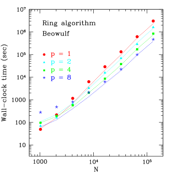
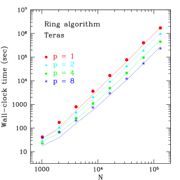
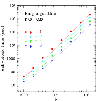
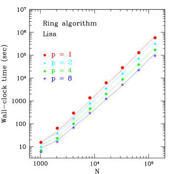
Figure 5: Wall-clock time as a function of the number of particles for the ring algorithm with blocking communication on the different architectures. The symbols represent the data obtained from the timing measurements while the dotted lines represent the predictions by the performance model.

The symbols represent the data obtained from the timing measurements while the dotted lines represent the predictions by the theoretical model. The particles are initially distributed in space according to a Plummer model with equal mass stars in virial equilibrium and the integration is for one $N$-body time-unit. The ring and the copy algorithm have a similar performance in terms of total execution time for large numbers of particles, whereas the ring algorithm is heavily dominated by communication for small numbers of particles. Like in the case of the copy algorithm, the efficiency decreases for large numbers of processors, where the communication governs the general performance, but increases for large numbers of particles. The agreement between the model and the measured times is generally good, especially for large $N$.

If non-blocking communication is used for the ring algorithm [8], the total execution time for one full force calculation can be significantly reduced. The calculation time for one shift of the systolic loop is the same as in the blocking case: $T_{\rm calc,1shift}=\tau_{f}ns_{\rm max}\thinspace$. The communication time has two separate contributions, one from the transfer of the positions and velocities and one from the transfer of the accelerations and jerks. We define $\tau_{pv}$ as the time needed to send the position and the velocity vectors of one particle to another processor. Similarly, we define $\tau_{aj}$ as the time needed to send the acceleration and the jerk vectors of one particle to another processor. Since the two communications are taking place simultaneously, the total communication time is given by the maximum between the two: $T_{\rm comm,1shift}={\rm max}\left[T_{\rm comm,1},T_{\rm comm,2}\right]$, where $T_{\rm comm,1}=\tau_{l}+\tau_{pv}s_{\rm max}$ is the time needed to transfer the positions and velocities of the block of particles while $T_{\rm comm,2}=\tau_{l}+\tau_{aj}s_{\rm max}$ is the time needed to transfer the accelerations and jerks of the same block. At the end of the last shift an additional communication is required $T_{\rm comm,final}=T_{\rm comm,2}\thinspace$. After $p$ shifts in the ring the total time to compute the force on the block of $s$ particles is

$$T_{\rm force}={\rm max}\left[T_{\rm calc,1shift},T_{\rm comm,1shift}\right]p+T_{\rm comm,final}\thinspace.$$ (8)

The use of non-blocking communication is efficient whenever the communication time is not negligible compared to the calculation time. For moderately concentrated models like the Plummer model this happens for small numbers of particles, when the average block size is small and hence the particles are less likely to be evenly distributed (see Fig. 6).

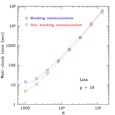
Figure 6: Timing comparison between the blocking and non-blocking communication ring algorithm. The runs were performed on the Lisa cluster with $p=16$ using a Plummer model and the integration time was one $N$-body time-unit in all cases. The symbols represent the data obtained from the timing measurements while the dotted lines represent the predictions by the performance model. For small $N$ the non-blocking scheme reduces the execution time by about a factor two, presenting an almost linear scaling. For larger $N$, where the total time is dominated by the force computation, both schemes present an $O(N^{2})$ scaling with the number of particles and achieve a similar performance.

5 Performance on the BlueGene/L supercomputer

The BlueGene/L supercomputer is a novel machine developed by IBM to provide a very high number of computing nodes with a modest power requirement. Each node consists of two processors, a special variant of IBM’s Power family, with a clock speed of 700 Mhz. To obtain good performance at this relatively low frequency, each node processes multiple instructions per clock cycle. The nodes are interconnected through multiple complementary high-speed low-latency networks, including a 3D torus network and a combining tree network.

We could perform a limited number of test runs on the Blue Gene/L machine hosted by the IBM Watson research center. We evolved an $N$=32768 Plummer model for a time $t$ = 0.03125 time-units using the block time-step code parallelized with the non-blocking ring algorithm. The execution times on 32, 64, 128 processors were 320 sec, 256 sec, 222 sec, respectively. Consequently, the speedup on 64 and 128 processors, relative to 32 nodes, was of only 1.25 and 1.5 respectively. We realized that a block time-step code is not efficient for a combination of a relatively small number of particles and a large number of processors. We then evolved a $N$=131072 Plummer model for one time-step using a shared time-step code parallelized with the ring algorithm. In Fig. 7 we show the timing results, together with the predictions by the theoretical model, as a function of the number of processors. An almost linear speedup is achieved by means of an efficient use of both processors in a node [16], with a peak speed of 2.8 GFlop/s per node. The theoretical model for a shared time-step code, which is based on Eq. (7), provides a very accurate prediction of the execution time for the following set of parameters: $\tau_{f}=1.5\times 10^{-7}\,s$, $\tau_{l}=5.0\times 10^{-6}\,s$, $\tau_{c}=1.0\times 10^{-5}\,s$.

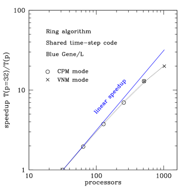
Figure 7: BlueGene/L speedup over 32 nodes in the case of the integration of a $N$=131072 Plummer model with a shared time-step code for one step. The full dots are the results for the Coprocessor mode (CPM) while the full square is the result for the Virtual Node Mode (VNM) (see [16] for technical details). The dotted line represents the prediction by Eq. (7).

These short test runs show that the Blue Gene/L supercomputer can achieve good performance and almost optimal speedup under conditions of good load balance.

6 Performance analysis on the GRID

Grid technology is rapidly becoming a major component of computational science. It offers a unified means of access to different and distant computational resources, with the possibility to securely access highly distributed resources that scientists do not necessarily own or have an account on. Connectivity between distant locations, interoperability between different kinds of systems, and resources and high levels of computational performance are some of the most promising characteristics of the Grid. Although significant improvement in the performance of direct codes can be obtained by means of general purpose parallel computers (see $\S$ 4), the use of highly distributed clusters within computational grids has not yet been explored.

In this section we present the results of experiments conducted on computational grids using the $N$-body code parallelized with a systolic algorithm and the MPICH-G2 device across large geographical distances. We explore the total effects of network latency on the performance on the 5-cluster DAS-2 Grid, distributed within the Netherlands and running the Globus toolkit [17], as well as on the 18-node CrossGrid testbed, distributed across Europe and running LCG2.

The MPI implementation that is used in a Globus environment is MPICH-G2, which is a grid-enabled implementation of the standard MPI v1.1. Using services from the Globus Toolkit, MPICH-G2 allows one to couple multiple machines, potentially of different architectures, to run MPI applications. It automatically converts data in messages sent between machines of different architectures and supports multi-protocol communication by automatically selecting TCP for inter-machine messaging and vendor-supplied MPI for intra-machine messaging.

We now describe the two grid testbeds used for our experiments.

6.1 The DAS-2 and CrossGrid testbeds

The Distributed ASCI Supercomputer (DAS-2) is a wide-area parallel computer which consists of clusters of workstations distributed across the Netherlands. The DAS-2 virtual machine is used for research on parallel and distributed computing by five Dutch universities and contains 200 computing nodes in total. Each node contains two 1 GHz Pentium IIIs, at least 1 GB RAM and a 20 GB local IDE disk. The nodes within a local cluster are connected by a Myrinet-2000 network, which is used as high-speed interconnection, while Fast Ethernet is used as OS network. The five local clusters are connected by Surfnet, the Internet backbone for wide-area communication across universities in the Netherlands. The version of MPICH-G2 available on DAS-2 is MPICH-GM, which uses Myricom’s GM as its message passing layer on Myrinet.

6.2 The CrossGrid testbed

The CrossGrid pan-European distributed testbed shares resources across 16 European sites. The sites range from relatively small computing facilities in universities to large research computing centers, offering an ideal mixture to test the possibilities of an experimental Grid framework. National research networks and the high-performance European network, Geant [18], assure inter-connectivity between all sites. The network includes a local step via Fast or Gigabit Ethernet, a jump via a national network provider at speeds that will range from 34 Mbits/s to 622 Mbits/s or even Gigabit and a link to the Geant European network at 155 Mbits/s to 2.5 Gbits/s. The platforms include Intel Pentium III and Intel Xeon processors with speeds ranging from 1 to 2.4 GHz.

The CrossGrid team focuses on the development of Grid middle-ware components, tools, and applications with a special focus on parallel and interactive computing, deployed across 11 countries. The added value of this project consists in the extension of the Grid to support interactive applications. The CrossGrid testbed largely benefits from the European Data Grid [19] experience on testbed setup and Globus middle-ware distributions.

6.3 Performance results

As shown in $\S$ 4, the main factors determining the general performance of a parallel application are the calculation speed of each node, the bandwidth of the inter-processor communication and the network latency. In the case of a computational grid, the latency between different clusters and the slower network may sensibly affect the execution times.

Adopting the same nomenclature as in $\S$ 4.1 and 4.2, we derive a theoretical estimate for the time $T_{\rm force}$ in the most general case of a heterogeneous grid, where each processor has a different CPU speed and any pair of processors is interconnected by a different network. In the case of the ring algorithm with blocking communication the total time after one shift is given by $T_{\rm force,1shift}=\max_{i=1\dots p}\left\{\tau_{f,i}~{}n~{}s_{i}\right\}+\max_{i=1\dots p}\left\{\tau_{l,i}+\tau_{c,i}~{}s_{i}\right\}$, where the subscript $i$ refers to processor $i$. Taking into account the fact that each processor may have a different block size $s_{i}$, the total time needed for the computation of the forces exerted on the block of $s$ particles can be written as

$$T_{\rm force}=\sum_{shift=1}^{p}n~{}\max_{i=1\dots p}\left\{\tau_{f,i}~{}s_{i}\right\}+\sum_{shift=1}^{p}\max_{i=1\dots p}\left\{\tau_{l,i}+\tau_{c,i}~{}s_{i}\right\}~{}.$$ (9)

In the ideal case of all processors having the same block size $s_{i}=s/p$, the previous equation simplifies to

$$T_{\rm force}=N~{}\frac{s}{p}\max_{i=1\dots p}\left\{\tau_{f,i}\right\}+p~{}\max_{i=1\dots p}\left\{\tau_{l,i}+\tau_{c,i}~{}\frac{s}{p}\right\}~{}.$$ (10)

To measure the effect of latency we performed several test runs on the DAS-2 low latency supercomputer and the CrossGrid testbed using the systolic $N$-body code. The specifications for the DAS-2 [20] and for the CrossGrid are shown in Table 2.

Table 2: Specifications for the grid testbeds.

	CPU	Network	$\tau_{f}$ [sec]	$\tau_{l}$ [sec]	$\tau_{c}$ [sec]
DAS-2	1 GHz	Surfnet	4.5$\times 10^{-7}$	5.0$\times 10^{-5}$	8.0$\times 10^{-4}$
CrossGrid	1 GHz	Geant	4.5$\times 10^{-7}$	2.0$\times 10^{-3}$	4.0$\times 10^{-3}$

We evolved the same initial configuration (Plummer model) for one $N$-body time-unit using 4 processors.

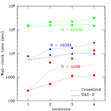
Figure 8: Performance comparison of the direct $N$-body code parallelized with the ring algorithm on the DAS-2 wide-area supercomputer (dashed lines) and the CrossGrid distributed testbed (dotted lines). The wall-clock time is plotted as a function of the number of locations where the computing nodes are selected. The timing refers to the integration of a Plummer model for N=4096 (full dots), 16384 (full triangles), 65536 (full squares), for one $N$-body time-unit. The dotted and dashed lines indicate the predictions by the performance model Eq. (9) .

The total execution time is plotted in Fig. 8 as a function of the number of different locations hosting the computing nodes. The low latency network on the DAS-2 generally results in a good performance even if the nodes are allocated in different clusters. Only in the case of a very small number of particles, like for the $N$ = 4096 run, the execution time increases steadily with the number of locations. This is due to an unfavorable computation to communication ratio for small $N$. The effects of inter-process communication are more evident for the CrossGrid runs, where the execution time increases substantially with the number of locations. However, the performance improves as the size of the $N$-body system increases since the computation to communication ratio becomes higher and a better load balance can be achieved. For large systems, the performance on the CrossGrid is at most a factor three worse than that on DAS-2. The performance model can predict the execution time for DAS-2, which is an homogeneous system, while can only reproduce the behavior of the CrossGrid for large $N$, when the calculation dominates over communication. Even though the clusters have been selected to be as similar as possible, the CrossGrid is not an homogeneous system and the different distances between the locations result in different communication times.

7 Discussion

A numerical challenge for the astronomical community in the next years will be the simulation of star clusters containing one million stars. We have shown that direct $N$-body codes can efficiently be applied to the simulation of large stellar systems and that their performance can be predicted with simple models.

In this section, we apply the performance model introduced in § 4.1 for the copy algorithm to predict the total execution time for the simulation of a system with $N=10^{6}$. In Table 3 we report our predictions for the execution times in the simulation of such a star cluster. For the prediction we consider the parameters of current state-of-the-art supercomputers (Lisa and BlueGene) and of an expected state-of-the-art supercomputer in ten years time (Future). For the Future computer we consider the Lisa cluster as a reference and we assume that the CPU speed doubles every 18 months the network speed doubles every 9 months. The resulting parameters for the Future computer are $\tau_{f}=2.0\times 10^{-9}$, $\tau_{c}=1.0\times 10^{-6}$ and $\tau_{l}=5.0\times 10^{-7}$.

Table 3: Predicted execution time for a star cluster.

System	N	$p_{\rm min}$	time (1 $N$-body unit)	time (1000 $N$-body units)
Lisa	$10^{6}$	1000	1.3 days	3.5 years
BlueGene	$10^{6}$	1000	1.0 day	3.1 years
Future	$10^{6}$	1000	30 min	12 days

We find that a typical supercomputer in ten years will be able to simulate a star cluster (one million stars) for one $N$-body time-unit in about thirty minutes using 1000 processors. A full simulation of 1000 $N$-body units will thus require less than a month to complete. Large supercomputers containing at least 1000 processors will be necessary to perform the first realistic simulation of a large globular clusters. Algorithmic developments are unlikely to result in a reduction of the calculation time as the $N^{2}$ operation will always remain the most demanding part of a simulation using a direct code. On the other hand, new treatments of the additional physics involved in a realistic simulation (stellar and binary evolution, dynamical encounters, collisions between stars) will be very important for future comparisons between observations and simulations of star clusters.

The simulation of larger systems like galactic nuclei ($10^{9}$ stars) or galaxies ($10^{11}$ stars) will be unrealistic to perform on a large supercomputer, even with future special purpose hardware. The best method for this objective is the use of hybrid codes in which a direct integration is combined with less accurate but faster techniques, like Monte Carlo codes or tree codes. The different dynamical evolution of large systems like galaxies, which can be considered “non-collisional”, will allow for the partial use of approximated methods without loss of fundamental physical phenomena.

8 Conclusions

We have implemented two parallelization schemes for direct $N$-body codes with block time-steps, the copy and ring algorithm, and compared their performance on different parallel computers. In the case of clusters or supercomputers, the execution times for the two schemes are comparable except for very small systems where the communication time dominates over the calculation time and hence the copy algorithm performs slightly better. The ring algorithm is well suited for the integration of very large systems, because of its reduced memory demands, and for very concentrated models, where the average block size becomes very small and the algorithm can be implemented with non-blocking communication to limit the effects of load imbalance.

The timing experiments we have conducted on two Grid testbeds indicate that the performance on large grids is not significantly worsened by the communication among nodes residing in different locations, provided that the size of the $N$-body system is sufficiently large to ensure a high computation to communication ratio and a good load balance. Although these results are only preliminary, they appear very promising in the direction of ever larger $N$-body simulations of star clusters.

We have developed a performance model for each parallel scheme and we have applied it to the prediction of the execution time for the simulation of a star cluster containing one million stars. We expect such simulation to become feasible on a supercomputer in ten years. Simulating entire galaxies however is not foreseeable in the near future without major software developments.

9 Acknowledgments

We thank Jun Makino and Piet Hut for support through the ACS project (http://www.artcompsci.org). We also thank Gyan Bhanot, Bob Walkup and the IBM T.J Watson Research Center for performing test runs on the BlueGene supercomputer, the DAS-2 and CrossGrid projects, for their technical help in the grid tests and Rainer Spurzem and David Merritt for useful discussions on parallel computing. This work was supported by the Netherlands Organization for Scientific Research (NWO grant #635.000.001), the Royal Netherlands Academy of Arts and Sciences (KNAW) and the Netherlands Research School for Astronomy (NOVA).

References

- [1] H. Cohn, Late core collapse in star clusters and the gravothermal instability, ApJ, 242, (1980) 765.
- [2] B. W. Murphy, H. N. Cohn, R. H. Durisen, Dynamical and luminosity evolution of active galactic nuclei - Models with a mass spectrum, ApJ, 370, (1991) 60.
- [3] P. D. Louis, R. Spurzem, Anisotropic gaseous models for the evolution of star clusters, MNRAS, 251, (1991) 408.
- [4] M. Hénon, Two Recent Developments Concerning the Monte Carlo Method, in: IAU Symp. 69: Dynamics of the Solar Systems, 1975, p. 133.
- [5] L. Spitzer, Dynamical Theory of Spherical Stellar Systems with Large N (invited Paper), in: IAU Symp. 69: Dynamics of the Solar Systems, 1975, p. 3.
- [6] M. Giersz, Monte Carlo simulations of star clusters - I. First Results, MNRAS, 298, (1998) 1239.
- [7] J. Makino, T. Fukushige, M. Koga, Namura, GRAPE-6: Massively-Parallel Special-Purpose Computer for Astrophysical Particle Simulations, PASJ, 55, (2003) 1163.
- [8] E. N. Dorband, M. Hemsendorf, D. Merritt, Systolic and hyper-systolic algorithms for the gravitational N-body problem, with an application to Brownian motion, J. Computat. Phys., 185, (2003) 484.
- [9] J. Makino, S. J. Aarseth, On a Hermite integrator with Ahmad-Cohen scheme for gravitational many-body problems, PASJ, 44, (1992) 141.
- [10] J. Makino, P. Hut, Performance analysis of direct N-body calculations, ApJ Supplement, 68 (1988) 833.
- [11] S. L. W. McMillan, in: in The Use of Supercomputers in Stellar Dynamics, 1986, p. 156.
- [12] J. Makino, An efficient parallel algorithm for direct summation method and its variations on distributed-memory parallel machines, NewA, 7, (2002) 373.
- [13] D. C. Heggie, R. D. Mathieu, Standardised Units and Time Scales, LNP Vol. 267: The Use of Supercomputers in Stellar Dynamics (1986) 233.
- [14] H. C. Plummer, On the problem of distribution in globular star clusters, MNRAS, 71 (1911) 460.
- [15] J. Makino, A Modified Aarseth Code for GRAPE and Vector Processors, PASJ, 43, (1991) 859.
- [16] G. Almasi, et al., Unlocking the Performance of the BlueGene/L Supercomputer, SC2004 conference.
- [17] I. Foster, C. Kesselman, A Metacomputing Infrastructure Toolkit, Intl. Journ. Supercomputer Applications 11(2), (1997) 115.
- [18] M. Campanella, Implementation architecture specification for the Premium IP service, GN1 (GEANT) Deliverable D9.1-Addendum1.
- [19] I. Foster, C. Kesselman, S. Tuecke, The Anatomy of the Grid: Enabling Scalable Virtual Organizations, Intl. Journ. Supercomputer Applications 15(3) (2001) 1.
- [20] K. A. Iskra, G. D. van Albada, P. M. A. Sloot, Time Warp cancellation optimisations on high latency networks, in: Proceedings of the 7th IEEE International Symposium on Distributed Simulation and Real-Time Applications, Delft, The Netherlands, 2003, p. 128.