Dynamical modelling of stars and gas in NGC 2974:
determination of mass-to-light ratio, inclination and
orbital structure by Schwarzschild’s method

Abstract

We study the large-scale stellar and gaseous kinematics of the E4 galaxy NGC 2974, based on panoramic integral-field data obtained with SAURON . We quantify the velocity fields with Fourier methods (kinemetry), and show that the large-scale kinematics is largely consistent with axisymmetry. We construct general axisymmetric dynamical models for the stellar motions using Schwarzschild’s orbit-superposition method, and compare the inferred inclination and mass-to-light ratio with the values obtained by modelling the gas kinematics. Both approaches give consistent results. However we find that the stellar models provide fairly weak constraints on the inclination. The intrinsic orbital distribution of NGC 2974, which we infer from our model, is characterised by a large-scale stellar component of high angular momentum. We create semi-analytic test models, resembling NGC 2974, to study the ability of Schwarzschild’s modelling technique to recover the given input parameters (mass-to-light ratio and inclination) and the distribution function. We also test the influence of a limited spatial coverage on the recovery of the distribution function (i.e. the orbital structure). We find that the models can accurately recover the input mass-to-light ratio, but we confirm that even with perfect input kinematics the inclination is only marginally constrained. This suggests a possible degeneracy in the determination of the inclination, but further investigations are needed to clarify this issue. For a given potential, we find that the analytic distribution function of our test model is well recovered by the three-integral model within the spatial region constrained by integral-field kinematics.

1 Introduction

The internal dynamical structure of galaxies retains evidence of their evolution. The internal dynamics, however, can only be interpreted through a combination of observational and theoretical efforts. From a theoretical point of view, one wants to know how the stars are distributed in space and what velocities they have. From the observational point of view, one wants to determine the intrinsic structure of the observed galaxies. The goals of both approaches are equivalent, and consist of the recovery of the phase-space density, or distribution function (DF) of galaxies, which uniquely specifies their properties. An insight into the DF is possible by the construction of dynamical models which are constrained by observations. There are several modelling methods established in the literature, of which Schwarzschild’s orbit-superposition method is perhaps the most elegant (Schwarzschild, 1979, 1982). In the past few years it has been applied successfully to a number of galaxies (van der Marel et al., 1998; Cretton & van den Bosch, 1999; Cappellari et al., 2002; Gebhardt et al., 2003); but recent observational advances in spectroscopy with integral-field units offer for the first time full two-dimensional constraints on these dynamical models (Verolme et al. 2002; Copin, Cretton & Emsellem 2004).

This paper presents a case study of the early-type galaxy NGC 2974. It is one of the few elliptical galaxies known to contain an extended disc of neutral hydrogen in regular rotation (Kim et al., 1988). It also hosts extended H$\alpha$ emission (Buson et al., 1993; Plana et al., 1998), and belongs to the ‘rapid rotators’ (Bender, 1988). The total absolute magnitude of $M_{B}=-20.32$ puts NGC 2974 near the transition between giant ellipticals and the lower-luminosity objects which often show photometric and kinematic evidence for a significant disc component (e.g. Rix & White, 1992). Emsellem et al. (2003, hereafter EGF03), combining WFPC2 imaging with TIGER integral-field spectroscopy of the central few arcseconds, discovered a spiral structure in the H$\alpha$ emission in the inner few arcseconds, and concluded that the galaxy contains a inner stellar bar. The general properties of NGC 2974 are listed in Table 1.

The availability of both stellar and gaseous kinematics makes NGC 2974 a very interesting case for detailed dynamical modelling. Cinzano & van der Marel (1994) made dynamical Jeans models of the gaseous and stellar components additionally introducing a stellar disc in order to fit their long-slit data along three position angles. They found that the stellar and gaseous discs were kinematically aligned and the inclination of both discs was consistent with 60°. This prompted them to suggest a common evolution, where the gas could be ionised by the stars in the stellar disc. Using more sophisticated two-integral axisymmetric models, which assume the DF depends only on the two classical integrals of motion, the energy $E$ and the angular momentum with respect to the symmetry axis $L_{z}$, EGF03 were able to reproduce all features of Cinzano & van der Marel (1994) data as well as their integral-field TIGER data (covering the inner 4″). The models of EGF03 did not require a thin stellar disc to fit the data.

In this study we construct axisymmetric models for NGC 2974 based on Schwarzschild’s orbit superposition method. This method allows the DF to depend on all three isolating integrals of motion. All previous studies with three-integral models concentrated on the determination of the mass-to-light ratio $\Upsilon$, and mass of the central black hole, $M_{\rm BH}$. Based on the observed stellar velocity dispersion, the $M_{\rm BH}-\sigma$ relation (e.g. Tremaine et al., 2002) predicts a central black hole mass of $2.5\times 10^{8}M_{\odot}$, which at the distance of NGC 2974 (21.48 Mpc, Tonry et al. 2001) has a radius of influence of $0\aas@@fstack{\prime\prime}2$. Our observations of NGC 2974, with the integral-field spectrograph SAURON (Bacon et al., 2001), do not have the necessary resolution to probe the sphere of influence of the central black hole. The dynamical models presented here are therefore aimed at determination of the $\Upsilon$, the inclination, $i$, and the internal orbital structure. The stellar and gaseous kinematics also provide independent estimates of $\Upsilon$ and $i$, which can be used to cross-validate the results from the two approaches.

The results of the dynamical modelling are influenced by the assumptions of the models, but also by the specifics of the observations. The spatial coverage of the kinematics is one example. The two-dimensional coverage is an improvement over a few slits often used in other studies. Similarly, increasing the radial extent of the data could change the results. Another issue, associated with the modelling techniques, is the ability of the three-integral models to recover the true distribution function of the galaxy. This is very important for the investigation of the internal dynamics, since the recovered orbital distribution must represent the observed galaxy if we want to learn about the galaxy’s evolutionary history. In this paper we present tests designed to probe these issues and, in general, to determine the robustness of our three-integral method.

This paper is organised as follows. Section 2 summarises the SAURON spectroscopy and the photometric ground- and space-based data. The analysis of the velocity maps, used to quantify the presence and influence of possible non-axisymmetric motions as well as a brief discussion on bars in NGC 2974, is presented in Section 3. The three-integral dynamical models for the stellar motions are discussed in Section 4. Section 5 is devoted to tests of the three-integral method involving the determination of the model parameters ($\Upsilon$, $i$), influence of the radial extent of the data and the recovery of the DF. The modelling of the emission-line gas kinematics and comparison with the results of the stellar dynamical modelling is presented in Section 6. Section 7 concludes.

2 Observations and data reduction

The observations of NGC 2974 used in this work consist of ground- and space-based imaging, and ground-based integral-field spectroscopy. The imaging data were presented in EGF03 and the absorption-line kinematics of the SAURON observations in Emsellem et al. (2004, hereafter E04) as part of the SAURON survey (de Zeeuw et al., 2002). In this study we also use the SAURON emission-line kinematics of NGC 2974.

2.1 SAURON spectroscopy

NGC 2974 was observed with the integral-field spectrograph SAURON mounted on the 4.2-m William Herschel Telescope (WHT) in March 2001. The observations consisted of eight exposures divided equally between two pointings, each covering the centre and one side of the galaxy. The individual exposures of both pointings were dithered to obtain a better estimate of detector sensitivity variations and avoid systematic errors. The instrumental characteristics of SAURON and a summary of the observations are presented in Table 2.

The SAURON  data were reduced following the steps described in Bacon et al. (2001) using the dedicated software XSauron developed at CRAL-Observatoire. The performed reduction steps included bias and dark subtraction, extraction of the spectra using a fitted mask model, wavelength calibration, low frequency flat-fielding, cosmic-ray removal, homogenisation of the spectral resolution over the field, sky subtraction and flux calibration. All eight exposures were merged into one data cube with a common wavelength range by combining the science and noise spectra using optimal weights and (re)normalisation. In this process we resampled the data-cube to a common spatial scale ($0\aas@@fstack{\prime\prime}8\times 0\aas@@fstack{\prime\prime}8$) with a resulting field of view of about $45\arcsec\times 45\arcsec$. The data cube was spatially binned to increase the signal-to-noise ($S/N$) ratio over the field, using the Voronoi 2D binning algorithm of Cappellari & Copin (2003). The targeted minimum $S/N$ was 60 per aperture, but most of the spectra have $S/N$ ratio high (e.g. [$S/N$]${}_{max}\approx 420$) and about half of the spatial elements remain un-binned. The final data cube of NGC 2974 and the detailed reduction procedure was presented in E04.

Table 1: Properties of NGC 2974.

$$\begin{array}[]{lr}\hline\cr$Parameter$&$Value$\\ \hline\cr\vskip 3.0pt plus 1.0pt minus 1.0pt\cr$Morphological type$&$E4$\\ $M$_{B}$ [mag]$&-20.46\\ $effective B-V [mag]$&1.00\\ $PA [degrees]$&42\\ $Distance Modulus [mag]$&31.66\\ $Distance scale [pc/arcsec]$&104.13\\ \vskip 3.0pt plus 1.0pt minus 1.0pt\cr\hline\cr\end{array}$$

Notes – Listed properties are taken from the Lyon/Meudon Extragalactic Database (LEDA). Distance modulus is from Tonry et al. (2001)

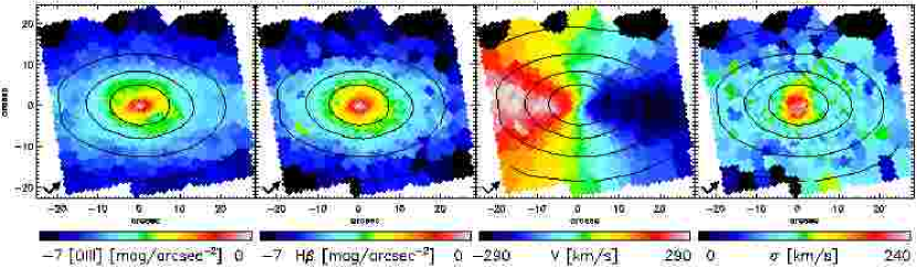
Figure 1: Distribution of H$\beta$ and [OIII] emission lines and gas kinematics observed by SAURON. Gas intensities are in mag arcsec^-2 with arbitrary zero points. Gas mean velocity V and velocity dispersion $\sigma$ are in $\>{\rm km}\,{\rm s}^{-1}$. Overplotted contours are levels of the reconstructed total intensity from the full SAURON spectra. Arrow in the left corner of each plot marks North-East orientation of the maps.

Table 2: The SAURON instrumental characteristics and exposure details of the observations of NGC 2974 obtained in March 2001 at the WHT. The sky apertures are pointed 1$\aas@@fstack{\prime}$9 away from the main field.

$$\begin{array}[]{ll}\hline\cr\vskip 3.0pt plus 1.0pt minus 1.0pt\cr$Field of view$&33\arcsec\times 41\arcsec\\ $Aperture size$&0\aas@@fstack{\prime\prime}94\\ $Final spatial sampling$&0\aas@@fstack{\prime\prime}8\\ $Spectral range$&4810-5300$\AA$\\ $Spectral sampling$&1.1$\AA\, pixel$^{-1}\\ $Spectral resolution$&4.2$\AA\, (FWHM)$\\ $\# of field lenses$&1431\\ $\# of sky lenses$&146\\ $\# of exposures$&8\\ $Exposure time per pointing$&1800\,$s$\\ $Instrumental dispersion$\,(\sigma)&108\>{\rm km}\,{\rm s}^{-1}\\ $Median seeing (FWHM)$&1\aas@@fstack{\prime\prime}4\\ \vskip 3.0pt plus 1.0pt minus 1.0pt\cr\hline\cr\end{array}$$

2.2 Absorption-line kinematics

The SAURON spectral range includes several important emission lines: H$\beta$, [OIII]$\lambda\lambda$4959,5007 and [NI]$\lambda\lambda$5198,5200 doublets. These lines have to be masked or removed from the spectra used for the extraction of the stellar kinematics. The method most suitable for this is the direct pixel-fitting method operating in wavelength space, which allows easy masking of the emission lines. We used the penalised pixel-fitting algorithm (pPXF) of Cappellari & Emsellem (2004), following the prescriptions of E04. The line-of-sight velocity distribution (LOSVD) was parametrised by the Gauss-Hermite expansion (van der Marel & Franx, 1993; Gerhard, 1993). The 2D stellar kinematic maps of NGC 2974, showing the mean velocity (V), the velocity dispersion ($\sigma$), as well as higher order Gauss-Hermite moments $h_{3}$ and $h_{4}$, were presented in E04, along with the kinematics of 47 other elliptical and lenticular galaxies. In this study we expand on the previously published kinematics by including two more terms in the Gauss-Hermite expansion ($h_{5}$ and $h_{6}$) to make sure all useful information was extracted from the spectra and tighten the constraints on the dynamical models. The extraction of additional kinematic terms was performed following the same procedure as in E04. The new extraction is consistent with the published kinematics (except that now the LOSVD is parameterised with 6 moments) and we do not present them here explicitly (but see Fig. 12).

We estimated the errors in the kinematic measurements by means of Monte-Carlo simulations. The parameters of the LOSVD were extracted from a hundred realisations of the observed spectrum. Each pixel of a Monte-Carlo spectrum was constructed adding a value randomly taken from a Gaussian distribution with the mean of the observed spectrum and standard deviation given by a robust-sigma estimate of the residual of the fit to the observed spectrum. All realisations provide a distribution of values from which $1\sigma$ confidence levels were estimated. During the extraction of the kinematics for error estimates, we switched off the penalisation of the pPXF method in order to obtain the true (unbiased) scatter of the values (see Cappellari & Emsellem 2004 for a discussion).

2.3 Distribution and kinematics of ionised gas

NGC 2974 has previously been searched for the existence of emission-line gas. Kim et al. (1988) reports the detection of HI in a disc structure aligned with the optical isophotes. The total mass of HI is estimated to be 8$\times 10^{8}\>{\rm M_{\odot}}$, rotating in a disc with an inclination of i $\approx$ 55°. Buson et al. (1993) detected H$\alpha$ emission distributed in a flat structure along the major axis. Assuming a disc geometry, the inferred inclination is $\approx$ 59°, and the total mass of HII was estimated to be $\approx$ 3$\times 10^{4}\>{\rm M_{\odot}}$. Similar results are found by Plana et al. (1998). Deep optical ground-based imaging studies suggested the existence of “arm-like” spiral structures, visible in the filamentary distribution of ionised gas outside $\sim 5\arcsec$ (Bregman et al., 1992; Buson et al., 1993). The recent high-resolution HST imaging in H$\alpha$+[NII] revealed the presence of a gaseous two-arm spiral in the inner $\sim 200$ pc, with a total mass of $6.8\times 10^{4}\>{\rm M_{\odot}}$ (EGF03).

The strongest emission line in the SAURON spectra of NGC 2974 is the [OIII] doublet. There is also considerable emission in H$\beta$ and some emission from the [NI] lines. Measurement of the emission-line kinematics followed the extraction of the absorption-line kinematics. For each spectrum in the data-cube we performed three steps:

• The pPXF method provided the model absorption spectrum that yielded the best fit to the spectral range with the emission lines ([OIII], H$\beta$ and [NI]) excluded.

• We then subtracted the model absorption spectrum from the original observed spectrum. This resulted in a “pure emission-line” spectrum which was used to extract the gas kinematics.

• Each emission line was approximated with a Gaussian. The fit was performed simultaneously to the three lines of [OIII] and H$\beta$, not using the mostly negligible [NI] doublet.

This procedure assumes that the velocity and velocity dispersion of the different emission lines are equal. Performing the simultaneous fit to the lines while allowing them to be kinematically independent yields similar results (Sarzi et al. in preparation). Following Osterbrock (1989) we assumed a 1:2.96 ratio for the components of the [OIII] doublet, while leaving the intensity of the [OIII] and H$\beta$ lines independent. The flux maps of [OIII] and H$\beta$ lines as well as the maps of the [OIII] emission-line mean velocity and velocity dispersion are presented in Fig. 1. The instrumental broadening of 108 $\>{\rm km}\,{\rm s}^{-1}$ was subtracted in quadrature from the emission-line velocity dispersion map presented here and also used in Section 6.

Both the H$\beta$ and [OIII] emission lines are present over the whole extent of the maps on Fig. 1, but their intensity drops off approximately exponentially with distance from the centre. The [OIII] emission is stronger over the entire SAURON field with the [OIII] to H$\beta$ line-ratio being $\approx$1.7. The shape of the distributions are very similar, although H$\beta$ follows the stellar light isophotes more precisely. The [OIII] distribution shows departures from the stellar isophotes in two roughly symmetric regions, positioned east and west of the centre on Fig. 1. The nature of these dips in the [OIII] flux are discussed in Section 3.3.

2.4 Ground- and space-based imaging

In this study we used the existing ground- and space-based images of NGC 2974. The already reduced wide-field ground-based I-band image of NGC 2974 was taken from Goudfrooij et al. (1994), obtained at the 1.0-m Jacobus Kapteyn Telescope (JKT). We also retrieved the Wide Field and Planetary Camera 2 (WFPC2) association images of NGC 2974 from the Hubble Space Telescope (HST) archive (Program ID 6822, PI Goudfrooij). The details of all imaging observations are presented in Table 3.

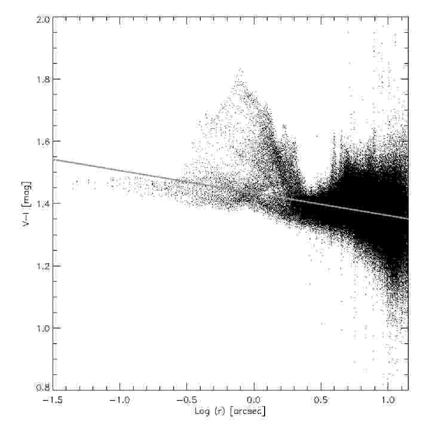
Figure 2: V-I colour versus the elliptical radius of every pixel in the inner 15″ of the WFPC2/PC1 images of NGC 2974. The straight line presents the best fit to the points obtained by minimising the absolute deviation. Notice the excess of red pixels between 0$\aas@@fstack{\prime\prime}$3 and 2$\aas@@fstack{\prime\prime}$5 caused by dust.

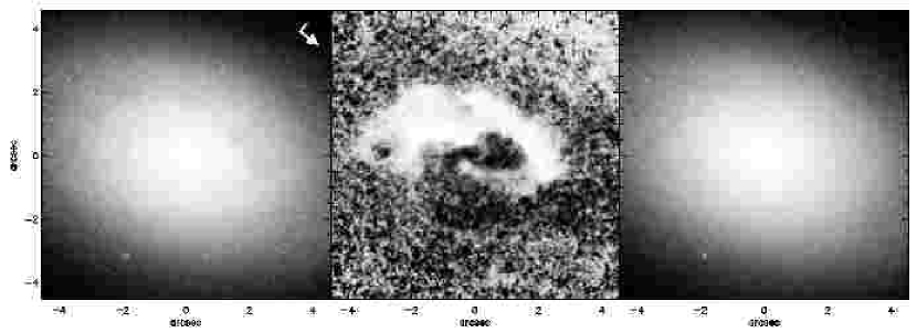
Figure 3: Dust correction on the F814W WFPC2 image of NGC 2974. From left to right: observed F814W image; colour excess E(V-I) obtained as described in the text; dust corrected F814W image. The arrow points to the north and associated dash to the east. All images were constructed using histogram equalisation. Lighter shades represent brighter regions. The E(V-I) map is stretched between -0.1 (dark) and 0.2 (bright) magnitudes.

Table 3: Summary of the ground- and space-based observations of NGC 2974. The exposure times of the HST/WFPC2 observations are averages of all frames used to produce the WFPC2 association images.

$$\begin{array}[]{lcc}\hline\cr\vskip 3.0pt plus 1.0pt minus 1.0pt\cr&$JKT$&$HST/WFPC2$\\ \vskip 3.0pt plus 1.0pt minus 1.0pt\cr\hline\cr\vskip 3.0pt plus 1.0pt minus 1.0pt\cr$Filter band$&I&$F$547$M$\,\&\,$F$814$W$\\ $Exposure time (s)$&60&700\,\&\,250\\ $Field of view (arcsec)$&380\times 350&32\times 32\\ $Pixel scale (arcsec) $&0.3106&0.0455\\ $Date of observations$&16.04.1993&16.04.1997\\ \vskip 3.0pt plus 1.0pt minus 1.0pt\cr\hline\cr\end{array}$$

A major complication in the derivation of the surface brightness model needed for the dynamical modelling is the existence of dust, clearly visible on the high resolution images. We considered two possible approaches: masking the patchy dust areas and excluding it from the calculation of the model, or constructing a dust-corrected image. We decided to adopt the latter approach to determine the stellar surface brightness. We derived the correction of dust absorption using the F547M and F814W WFPC2 images, following the steps listed in Cappellari et al. (2002). The process consists of construction of a colour excess map E(V-I), from a calibrated V-I colour image. The colour excess map is used to correct the pixels above a given E(V-I) threshold using the standard Galactic extinction curve. We assumed that the dust is a screen in front of the galaxy and that dust-affected pixels have the same intrinsic colour as the surrounding unaffected pixels. Figure 2 shows the calibrated V-I colour of pixels in the inner part of the PC images. The best fit to the colours was obtained by minimising the absolute deviation of the pixel values. This fit, represented by a line in Fig. 2, was used to calculate the colour excess by subtracting the measured colour from the fit. The resulting E(V-I) image is shown in the second panel of Fig. 3. The other panels on the same figure present the inner parts of the F814W PC image before and after the correction of dust absorption. The colour excess image highlights the dust structure visible also on Fig. 3 of EGF03 and suggests a non-uniform distribution of dust in the central region of NGC 2974.

3 Quantitative analysis of velocity maps

Two-dimensional kinematic maps offer a large amount of information and are often superior to a few long-slit velocity profiles. The two-dimensional nature of these data motivates us to quantify the topology and structure of these kinematic maps, just as is commonly done for simple imaging. We have developed a new technique to deal with kinematic maps based on the Fourier expansion, and, due to its similarity to the photometry, we named it kinemetry (Copin et al., 2001). This method is a generalisation of the approach developed for two-dimensional radio data (Franx et al., 1994; Schoenmakers et al., 1997; Wong et al., 2004). The aim of the method is to extract general properties from the kinematic maps of spheroidal systems (early-type galaxies) without assuming a specific intrinsic geometry (e.g. thin disc) for the distribution of stars. This changes the interpretation and the approach to the terms of the harmonic expansion from the case of cold neutral hydrogen or CO discussed in the above-mentioned papers. In this section we briefly present the method and apply it to the stellar and gaseous velocity maps (Krajnović et al. (in prep.)).

3.1 Harmonic Expansion

The kinemetry method consists of the straightforward Fourier expansion of the line-of-sight kinematic property $K(r,\theta)$ in polar coordinates:

$$K(r,\theta)=a_{0}(r)+\sum_{n=1}^{N}c_{n}(r)\,\cos[n(\theta-\phi_{n}(r))].$$ (1)

The expansion is done on a set of concentric circular rings (although other choices are possible), and its main advantage is linearity at constant $r$. The expansion is possible for all moments of the LOSVD, but in this paper we restrict ourselves to the mean velocity maps.

The kinematic moments (moments of LOSVD) of triaxial galaxies in a stationary configuration have different parity, e.g., mean velocity is odd, while the second moment $\langle v{{}^{2}}\rangle$, is even. The parity of a moment generates certain symmetries of the kinematics maps. More generally, the maps of odd moments are $point-anti-symmetric$, or:

$$V(r,\theta+\pi)=-V(r,\theta).$$ (2)

If axisymmetry is assumed, in addition to the previous relation, maps are $mirror-anti-symmetric$, or:

$$V(r,\pi-\theta)=-V(r,\theta),$$ (3)

These symmetry conditions translate into the requirement on the harmonic expansion (eq. 1) that for point-anti-symmetric maps the even coefficients in the expansion are equal to zero, while in the case of mirror-anti-symmetry, additionally, the odd phase angles have a constant value, equal to the photometric position angle (PA) of the galaxy in the case of a true axisymmetric galaxy. This means that to reconstruct the mean velocity map of a stationary triaxial galaxy, it is sufficient to use only odd terms in the expansion.

These properties of the velocity maps enable certain natural filtering (point-(anti)-symmetric — eq. (2), and mirror-(anti)-symmetric — eq. (3)) using the harmonic expansion with coefficients set to zero or phase angles fixed at certain values. For (visual) comparisons of the data with the results of axisymmetric modelling it is useful to apply the axisymmetric filtering to the data, as we will see below (Section 6).

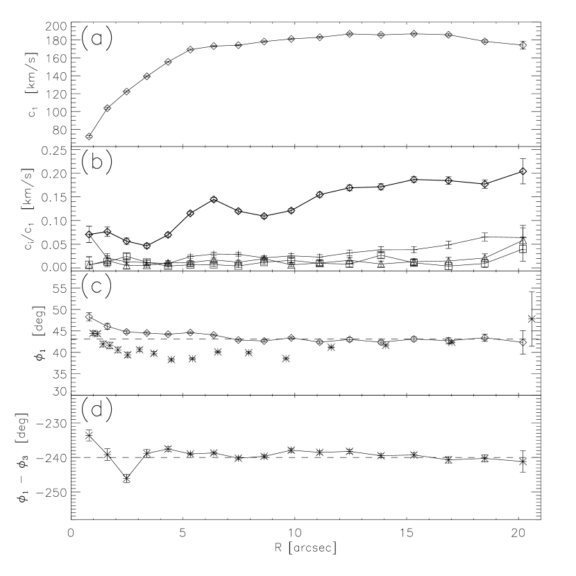
Figure 4: Kinemetric expansion of the stellar velocity field as a function of radius. From top to bottom: (a) first amplitude coefficient in the harmonic expansion c₁; (b) ratios of amplitude coefficients presented by: triangles c₂/c₁, diamonds c₃/c₁, squares c₄/c₁ and plusses c₅/c₁; (c) important position angles: phase angle $\phi_{1}$ representing the kinematic position angle (diamonds), photometric position angle as measured on WFPC2/PC1 F814W image (asterisks) and adopted value for photometric position angle measured from the integrated SAURON flux image (dashed straight line); (d) difference between the first and third phase from the kinemetric expansion.

3.2 Kinemetric analysis of velocity maps

We wish to know the intrinsic shape of NGC 2974 and, in particular, whether it is consistent with axisymmetry, which would permit the construction of three-integral axisymmetric dynamical models of the galaxy. In order to obtain the necessary information we applied the kinemetric expansion to the observed stellar velocity map. If NGC 2974 is an axisymmetric galaxy, the kinemetric terms should have odd parity (even terms should be zero) and the kinematic position angle should be constant and equal to the PA.

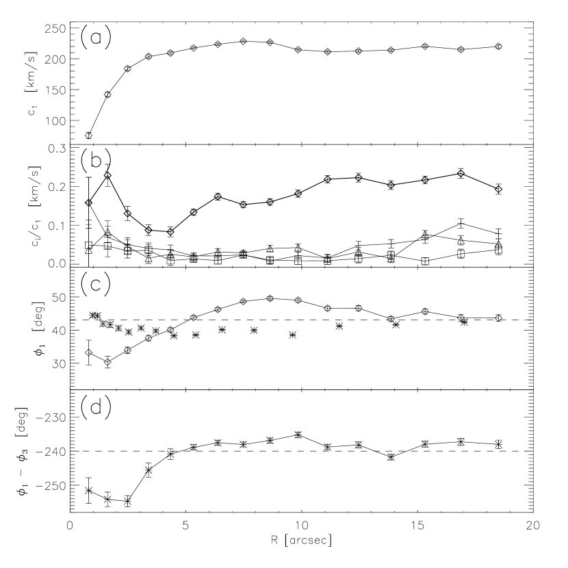
Figure 5: Same as Fig 4, but for the gas velocity map.

The amplitude and phases of the first five terms in the expansion are presented in Fig. 4. The first panel presents the dominant term in the expansion, $c_{1}$, which gives the general shape and amplitude of the stellar velocity map. The correction to this term is given by the next significant term, $c_{3}$, which is already much smaller than $c_{1}$ and is presented in the second panel as a fraction of $c_{1}$. Even terms in the expansion, $c_{2}$ and $c_{4}$, are also plotted on the same panel, and are much smaller ($\sim 1\%$ of $c_{1}$). For comparison, the fifth term in the expansion, $c_{5}$, is also plotted and is larger than both $c_{2}$ and $c_{4}$. The SAURON  pixel size is $\sim 1\arcsec$ and measurement of higher-order terms at radii smaller than 2″cannot be trusted. Clearly, the velocity map in NGC 2974 can be represented by the first two odd terms in the expansion. Neglecting all higher terms results at most in a few percent error.

The lower two panels in Fig. 4 present the phases of the dominant terms. The $\phi_{1}$ phase is defined as the kinematic angle of the velocity map, here measured east of north. This angle is compared with measurements of two important angles: (i) the PA measured on the WFPC2/PC F814W dust-corrected image using the IRAF ellipse fitting task ellipse and (ii) the PA measured on the reconstructed SAURON flux image obtained by integrating the spectra in each bin. The agreement between the different angles measured on the SAURON observations is excellent, with slight departures in the inner 3″. The PA measured on the high resolution WFPC2 image suggests a small photometric twist in the inner 10″ of $\approx 3\degr$, which can be also seen in Fig. 10.

The phase angle $\phi_{3}$ is the phase of the third term in the kinemetric extraction. It is easy to show, if the galaxy is axisymmetric (requiring in eq. 1, K(r,$\theta$) = 0 for $\theta=\phi_{1}+\pi/2$), and the higher terms can be neglected, that the phases $\phi_{1}$ and $\phi_{3}$ satisfy the relation:

$$\phi_{1}-\phi_{3}=\frac{n\pi}{3}$$ (4)

where $n\in\mathbb{Z}$. The last panel in Fig. 4 shows this phase difference. The condition given by eq.( 4) is satisfied along the entire investigated range with a small deviation in the inner 3″. Summarising all the above evidence, we conclude that the observed stellar kinematics in NGC 2974 is consistent with axisymmetry.

We repeated the kinemetric analysis on the emission-line gas velocity maps and present the results in Fig. 5. While the amplitude coefficients, $c_{i}$, are similar to the stellar coefficients (small values of all terms higher than $c_{3}$), the behaviour of the phase angles is quite different.

The last panel of Fig. 5 is perhaps the best diagnostic tool. The dashed line presents the required value for the difference between the phase angles, $\phi_{1}-\phi_{3}$, assuming axisymmetry. Deviations are present in the inner $4\arcsec$ and, although much smaller, between $9\arcsec$ and $11\arcsec$. These deviations indicate departures from axisymmetry, which are strongest in the central few arcsecs.

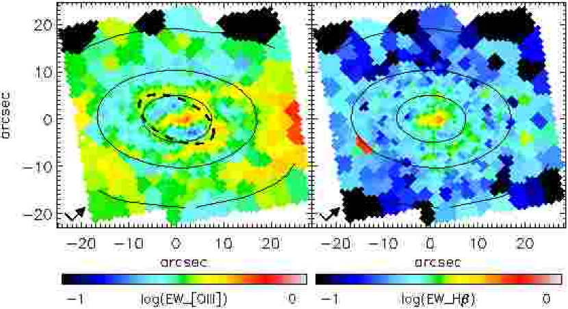
Figure 6: Equivalent widths of [OIII] and H$\beta$ emission-lines. These plots, constructed by dividing the emission-line flux by the symmetrised stellar continuum, show the relative distribution of emission-lines to the stellar continuum. The dashed ellipse represents the possible OLR ring of the inner bar (see text for details). Overplotted contours are levels of the reconstructed total intensity from the full SAURON spectra. The arrow in the left corner of each plot marks North-East orientation of the maps.

3.3 Signature of bars in NGC 2974

In the previous section, we quantified the signatures of non-axisymmetry on the gas velocity maps, especially strong in the inner $4\arcsec$. Inside this radius, EGF03 discovered a two-armed spiral and explained it by a weak bar with the corotation resonance (CR) at 4$\aas@@fstack{\prime\prime}$9 and outer-Lindblad resonance (OLR) at 8$\aas@@fstack{\prime\prime}$5. These scales are consistent with the observed departures from axisymmetry in the SAURON kinematic maps. An additional confirmation comes from the equivalent width maps of emission-lines (Fig. 6). These maps show the distribution of the emission-lines relative to the stellar continuum. Especially noticeable is the ring structure in the [OIII] equivalent width distribution. For comparison, we overplotted an ellipse with semi-major axis length of 8$\aas@@fstack{\prime\prime}$5 (the radius of OLR of the EGF03 bar). The orientation ($\sim 25\degr$ away from the major axis of the galaxy) and the size of the ring ($\sim 8\aas@@fstack{\prime\prime}5$) are in good agreement with the expected characteristics of the bar discovered by EGF03.

The equivalent width maps show that [OIII] emission-line is also influenced outside the OLR. There is an increase in the value of the equivalent width at larger radii as well as a filamentary (spiral) structure connecting the ring and this large scale region. Also, as seen before on Fig. 1, the distribution of the [OIII] emission-line intensity exhibits an elongated structure in the central 5″. Similarly, around $8\arcsec-10\arcsec$ [OIII] is also elongated, but this time approximately perpendicular to the first elongated structure. Following this, the [OIII] map has a plateau between 12″ and 15″. The end of the plateau is followed by a dip in the distribution with a possible turn up at radii larger than 20″.

Although the central structure and kinematics of the [OIII] distribution are influenced by the inner bar, the large-scale structure (beyond $\approx 10\arcsec$) is not likely to be influenced by this weak inner bar. On a more speculative basis, we can infer the existence of a large-scale bar. Studies of double bars (Erwin & Sparke, 2002; Laine et al., 2002; Erwin & Sparke, 2003) suggest a size ratio of about 5 to 10 between the primary and secondary bars; this would set the size of an hypothetical large-scale (primary) bar in NGC 2974 to between about $12\aas@@fstack{\prime\prime}5$ and $25\arcsec$.

Figure 7: Diagram of resonances in NGC 2974, derived from the potential of the best-fitting stellar dynamical model. The upper horizontal line is the pattern speed of the nuclear (secondary) bar from the EGF03 study ($\Omega^{s}_{p}=700\>{\rm km}\,{\rm s}^{-1}$ kpc^-1). The lower horizontal line shows the position of the inferred pattern speed of the large-scale primary bar ($\Omega^{p}_{p}=185\>{\rm km}\,{\rm s}^{-1}kpc^{-1}$). The vertical lines show the assumed radial positions of important resonances of the primary bar. From left to right: ILR (CR of the secondary bar), UHR, CR and OLR.

A more precise, although still approximate, estimate of the properties of the primary bar can be obtained from the resonance curves of NGC 2974. Using the potential of the best-fitting stellar dynamical model (see Section 4) we constructed the resonance diagram presented in Fig. 7. We calculated profiles of $\Omega$, $\Omega-\kappa/2$, $\Omega+\kappa/2$ and $\Omega-\kappa/4$, where $\Omega$ is the angular velocity, $V/r$, and $\kappa$ is epicyclic frequency, defined as $\kappa^{2}=r\frac{\mathrm{d}\Omega^{2}}{\mathrm{d}r}+4\Omega^{2}$. Assuming that the resonances of the primary and the secondary bar are coupled to minimise the chaos produced around the resonances (Friedli & Martinet, 1993; Pfenniger & Norman, 1990), where the inner Lindblad resonance (ILR) of the primary bar is the CR of the secondary bar, we can estimate the main resonances of the primary bar (indicated by the vertical lines on Fig. 7). The pattern speed of the primary component is then $\approx 185\>{\rm km}\,{\rm s}^{-1}$ kpc^-1, ILR is at $4\aas@@fstack{\prime\prime}9$, ultra harmonic resonance (UHR) at $\approx 12\aas@@fstack{\prime\prime}5$, CR at $\approx 18\aas@@fstack{\prime\prime}6$ and OLR at $\approx 27\aas@@fstack{\prime\prime}7$. The size of the primary bar can be taken to be 80% of its CR, so about 13 to 14″($\sim 1.4$ kpc).

The presented analysis is strictly valid only for an axisymmetric potential with a weak bar perturbation, hence the above-mentioned size estimates are only approximate, but indicative. We see several features in the [OIII] distribution and velocity maps that support the assumption of a large-scale primary bar: the dip in the gas velocity map around 12″, the plateau between 12″and 15″in the [OIII] distribution as well as the dip in the [OIII] distribution around 18″. The last one corresponds to the position of the CR, which is a chaotic region devoid of gas, consistent with the observed lower flux in that region.

3.4 Case for axisymmetry in NGC 2974

The alignment of the gaseous and stellar component, previously detected and also confirmed in this study, suggests that NGC 2974 is an axisymmetric galaxy. However, the gaseous component shows signatures of non-axisymmetric perturbations. The contribution of the non-axisymmetric motion, $\Delta V/c_{1}$, to the total velocity field can be quantified from the phase difference $\phi_{3}-\phi_{1}$. If the condition in eq. (4) is not satisfied then:

$$\frac{\Delta V}{c_{1}}=\frac{c_{3}}{c_{1}}\sin 3(\phi_{1}-\phi_{3}),$$ (5)

which is presented in Fig. 8 for both stellar and gaseous velocity maps. At $\sim 3\arcsec$, $\Delta V/c_{1}$ for the emission-line gas is $\approx 0.1$ and at $\sim 10\arcsec$ it is $\approx 0.04$, confirming that the non-axisymmetric contribution is significant in the centre of the emission-line velocity map. Its influence on the stellar velocity is not significant over the SAURON  field. Emission-line gas is a more responsive medium and unlike the stars, due to the viscosity of the gas particles, shows evidence of weak non-axisymmetric perturbations. It is possible that other early-type galaxies with disc-like components harbour such weak and hidden bar systems.

Summarising, the stellar velocity map is point- and mirror-anti-symmetric, supporting an axisymmetric shape for NGC 2974. On the other hand, the gaseous velocity map shows strong deviations from mirror-anti-symmetry in the centre, and the distribution and equivalent width of [OIII] emission lines supports the weak inner bar found by EGF03 and suggests the existence of a weak large-scale bar. However, since the bar perturbations on the axisymmetric potential are presumed to be weak and appear do not influence the stellar kinematics, we ignore them in the remainder of the paper, and describe NGC 2974 with an axisymmetric potential.

Figure 8: Contribution of the non-axisymmetric motion to the stellar and gaseous velocity fields, as a fraction of the dominant term in the kinemetric expansion, $c_{1}$. Diamonds represent the emission-line gas velocity contribution, while triangles denote the stellar velocity contribution.

4 Stellar Dynamical Modelling

In order to investigate the orbital structure of NGC 2974 we construct fully general axisymmetric models of the galaxy’s stellar component. The three-integral models presented here are based on Schwarzschild’s orbit superposition method (Schwarzschild, 1979, 1982), further developed by Rix et al. (1997), van der Marel et al. (1998) and Cretton et al. (1999), and adapted for more general surface-brightness distributions by Cappellari et al. (2002, hereafter C02) and Verolme et al. (2002, hereafter V02), similarly as in Cretton & van den Bosch (1999). The three-integral modelling technique is widely used for constructing dynamical models of axisymmetric galaxies, and has been thoroughly described in the literature by the aforementioned authors as well as by other groups (e.g. Gebhardt et al., 2003; Valluri et al., 2004). It is most commonly used to determine the masses of the central black holes in nearby galaxies and investigate the internal orbital structure of the galaxies. The SAURON observations of NGC 2974 do not have the necessary resolution to probe the sphere of influence of the central black hole and we therefore restrict ourselves to the determination of the mass-to-light ratio $\Upsilon$ and the inclination $i$ of the galaxy, as well as the internal orbital structure.

4.1 The Multi-Gaussian expansion mass model

The starting point of the stellar dynamical modelling is the determination of the gravitational potential of the galaxy. The potential can be obtained by solving the Poisson equation for a given density distribution which can be derived by deprojecting the observations of the 2D stellar surface density. In this work we used the multi-Gaussian expansion (MGE) method (Emsellem et al., 1994), following the approach of C02 and V02.

Table 4: The MGE parameters of the circular PSF of HST/WFPC2/F814W filter.

$$\begin{array}[]{ccc}\hline\cr\vskip 3.0pt plus 1.0pt minus 1.0pt\cr$j$&$G$_{j}&\sigma_{k}$(arcsec)$\\ \vskip 3.0pt plus 1.0pt minus 1.0pt\cr\hline\cr 1&0.352&0.024\\ 2&0.531&0.072\\ 3&0.082&0.365\\ 4&0.035&0.908\\ \vskip 3.0pt plus 1.0pt minus 1.0pt\cr\hline\cr\end{array}$$

Table 5: The parameters of the MGE model of the deconvolved I-band WFPC2 surface brightness of NGC 2974. Columns present (from left to right): number of the two-dimensional Gaussian, central intensity of the Gaussian, width (sigma) of the Gaussian, axial ratio of the Gaussian, total intensity contained in the Gaussian.

$$\begin{array}[]{ccccc}\hline\cr\vskip 3.0pt plus 1.0pt minus 1.0pt\cr$j$&$I$_{j}(L_{\odot}{pc}^{-2})&\sigma_{j}$(arcsec)$&$q$_{j}&$L$_{j}(\times 10^{9}L_{\odot})\\ \vskip 3.0pt plus 1.0pt minus 1.0pt\cr\hline\cr 1&190297.&0.0378596&0.580000&0.0108\\ 2&44170.6&0.0945030&0.800000&0.0215\\ 3&24330.8&0.185143&0.800000&0.0455\\ 4&27496.3&0.340087&0.583279&0.1264\\ 5&23040.6&0.591227&0.720063&0.3952\\ 6&10299.6&1.15500&0.777448&0.7279\\ 7&5116.29&3.41758&0.658664&2.6820\\ 8&1902.25&8.67562&0.597636&5.8305\\ 9&388.278&17.5245&0.677645&5.5060\\ 10&139.447&43.9864&0.580000&10.663\\ 11&16.9405&82.9488&0.800000&6.3538\\ \vskip 3.0pt plus 1.0pt minus 1.0pt\cr\hline\cr\end{array}$$

In order to get the MGE model, we simultaneously fitted the ground-based I-band image and the dust-corrected PC part of the WFPC2/F814W image using the method and software developed by Cappellari (2002). The dust correction (Section 2.4) successfully removed the dust contamination from the high-resolution image of the nucleus, but the large-scale image was badly polluted by several stars, with a particularly bright one almost on the galaxy’s major axis. We masked all stars inside the model area to exclude them from the fit. The ground-based image, used to constrain the fit outside 25″, was scaled to the WFPC2/PC1 image. We computed the PSF of the F814W PC1 image at the position of the nucleus of NGC 2974, using the TinyTim software (Krist & Hook 2001), and parametrised it by fitting a circular MGE model with constant position angle as in C02. Table 4 presents the relative weights G_j (normalised such that their sum is equal to unity) and the corresponding dispersions $\sigma$ of the four Gaussians. Table 5 gives the parameters of the MGE model analytically deconvolved from the PSF. Following the prescription of Cappellari (2002), we increased the minimum axial ratio of the Gaussians, q_j, until the $\chi^{2}$ significantly changed, in order to make as large as possible the range of allowed inclinations by the MGE model. The upper limit to the q_j was also constrained such that the MGE model is as close as possible to a density stratified on similar ellipsoids. Although the deprojection of an axisymmetric density distribution is non-unique (Rybicki, 1987), our ‘regularisation’ on the MGE model produce realistic intrinsic densities, while preventing sharp variations, unless they are required to fit the surface brightness. We verified that the MGE model used in this study is consistent with the MGE model presented in EGF03.

Figure 9: Left Panels: Comparison between the combined WFPC2/F814W and ground-based photometry of NGC 2974 (open squares) and the MGE model (solid line) in seven angular sectors as function of radius. The individual convolved Gaussians are also shown. Right panels: radial variation of the relative error along the profiles.

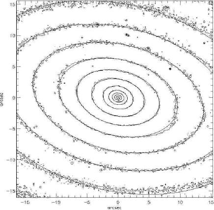
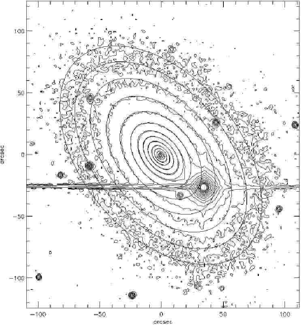
Figure 10: Contour maps of the ground-based I-band and dust-corrected WFPC2/F814W images. The brightest star on the ground-based image as well as four additional stars covered by the model were masked out and excluded from the fit. Superposed on the two plots are the contours of the MGE surface brightness model, convolved with the WFPC2 PSF.

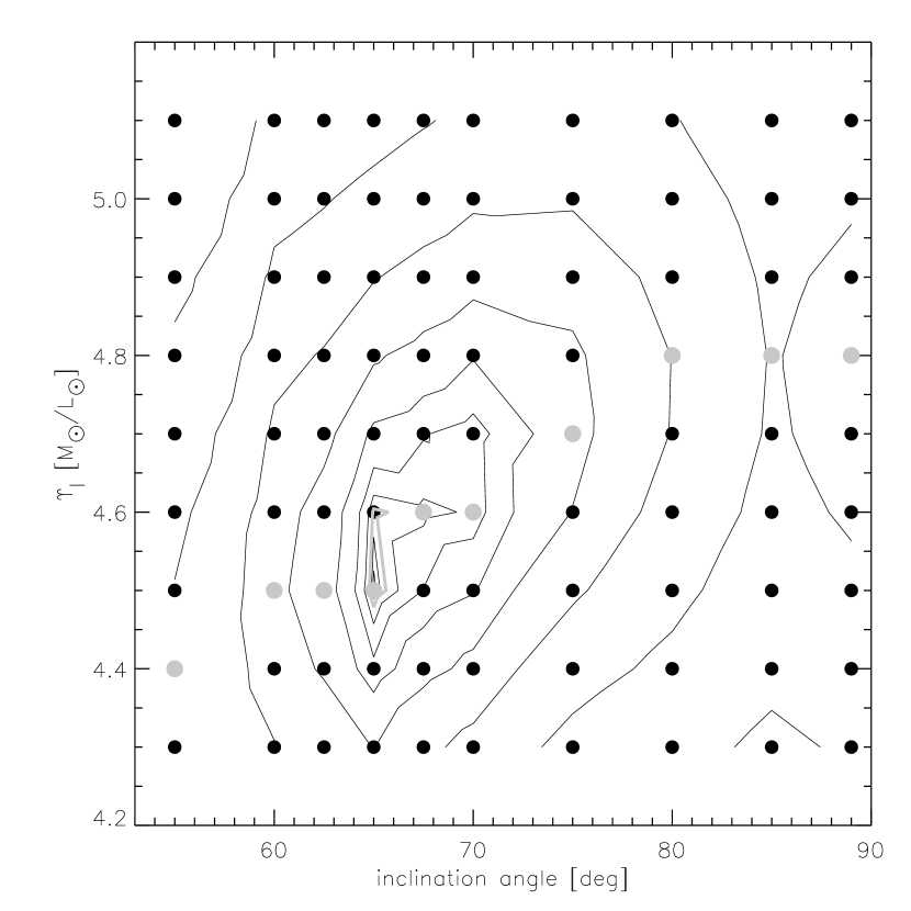
Figure 11: A grid of inclination angle $i$ versus $M/L$ ratio $\Upsilon$. Contours present constant $\Delta\chi^{2}$, measuring the goodness of fit of the dynamical models. Every symbol corresponds to a three-integral axisymmetric model with given inclination angle and $\Upsilon$ ratio. The best-fitting model for each inclinations are presented with grey symbols. The first three contours show the formal 68.3%, 95.4% and 99.73% (thick grey contour) confidence regions for two degrees of freedom. The best-fitting model on the grid has an inclination of 65°and $\Upsilon$ = 4.5.

The comparison between the MGE model and the photometry along different angular sectors is shown in Fig. 9. The profiles are reproduced to within 3%, and the RMS error is about 2%. The increase of the relative error (right-hand panel in Fig. 9) at larger radii is caused by the light pollution of the bright star on the major axis of the galaxy and can be better understood by looking at the comparison of the convolved model and the actual observation. Fig. 10 presents both ground- and space-based images and the MGE model. On the WFPC2/PC image there is a slight deviation from the model (of constant PA) about 10″ from the nucleus. The deviating structure is point-symmetric and reminiscent of a spiral perturbation. as suggested by other studies (Bregman et al. 1992; Buson et al. 1993; EGF03). Except for this slight departure from the model the galaxy surface brightness is well represented by the MGE model and we use it to calculate the representative gravitational potential.

4.2 Construction of three-integral models

Briefly, Schwarzschild’s method can be divided in four steps. In the first step, one derives the stellar potential assuming the shape of the potential (axisymmetry) and stellar mass-to-light ratio, $\Upsilon$ (free parameter), through deprojection of a parametrisation of the surface density (in this case MGE parametrisation which can be deprojected analytically). The second step involves the construction of a representative orbit library by integrating the orbits in the derived potential. Each orbit is specified by three integrals of motion ($E,L_{z},I_{3}$), where $E$ is the energy, $L_{z}$ the component of the angular momentum along the $z$ symmetry axis, and $I_{3}$ is a non-classical integral, which is not known analytically. The integral space is constructed on a grid that includes $>$99% of the total luminous mass of the galaxy. The next step consists of projecting the orbits onto the space of observables ($x^{\prime}$, $y^{\prime}$, $v_{los}$), where $(x^{\prime},y^{\prime})$ are in the plane of the sky and $v_{los}$ is the line-of-sight velocity given by the observations. In our implementation, this is done taking into account the PSF convolution and aperture binning. The final step of the method is to determine the set of weights for each orbit that, when added together, best corresponds to the observed kinematics in the given spatial bin as well as reproducing the stellar density. In our implementation of the method, this best-fitting set is found by solving a non-negative least-squares (NNLS) problem using the routine written by Lawson & Hanson (1974).

The software implementation used here is similar to that used in the V02 and C02 studies, but it has evolved substantially since. The improvements are described in detail in Cappellari et al. (in prep.). We verified that the results from the new code are the same as from the old one if identical settings are adopted. An application to the elliptical galaxy NGC 4473 was presented in Cappellari et al. (2004). Here we give a quick overview of the changes with respect to the description in C02:

1. The method requires that the orbits sample a three-dimensional space of integrals of motion, the energy $E$, $L_{z}$ and $I_{3}$. In the new scheme (see Cretton et al. 1999 for details of the previous approach), at each $E$, we construct a polar grid of initial starting positions on the meridional plane (linear in angle and in radius), going from $R=z=0$ to the curve defined by the thin tube orbits (to avoid duplication) which is well approximated by the equation $R^{2}+z^{2}=R^{2}_{c}(E)$, where $R_{c}(E)$ is the radius of the circular orbit at energy E. The orbits are released with $v_{R}=v_{z}=0$ and $L_{z}\neq 0$. In this way we sample the observable space by uniformly distributing the position of the orbital cusps (see Cappellari et al. 2004) on the sky plane.

2. Improved treatment of seeing effects and instrumental point spread function (PSF) by a Monte Carlo method. The PSF can be considered as the probability that an observed photon arriving at a detector will be displaced from its original position by a given amount (specified by the PSF characteristics). The projected orbital points (results of the orbit integration and projection onto the sky-plane) are stored in the apertures in which they landed after applying a random displacement taken from the Gaussian probability distribution defined by the PSF.

3. Generalisation of the projection of the orbits into the space of the observables. The bins of the optimal Voronoi binning of the two-dimensional integral-field data have non-rectangular shapes. The orbital observables now can be stored on apertures of any shape that can be represented by polygons.

4.3 Stellar dynamics - modelling results and discussion

Our stellar kinematic maps of NGC 2974 consist of 708 Voronoi bins. Each bin contributes with 6 kinematic observables to which we also add the intrinsic and projected mass density observables, resulting in a grand total of 5664 observables. The largest orbit library that was computationally possible for the given number of observables, consists of $2\times 41\times 10\times 10=8200$ orbits (for each of the 41 different $E$ we construct a polar grid of starting points sampling 10 angles and 10 radii). With this choice of orbit library, the number of observables is smaller than the number of orbits, and the NNLS fit will not have a formally unique solution. Moreover the recovery of the orbital weights for the orbits from the observations is an inverse problem, and as such is intrinsically ill-conditioned. For these reasons a direct solution of the problem generally consists exclusively of sharp isolated peaks. It is unlikely for the DF of real galaxies to be very jagged, since (violent) relaxation processes tend to smooth the DF. Moreover observational constraints on the smoothness of the DF, at least for the bulk of the stars in a galaxy, come from the smoothness of the observed surface brightness, down to the smallest spatial scales sampled by HST.

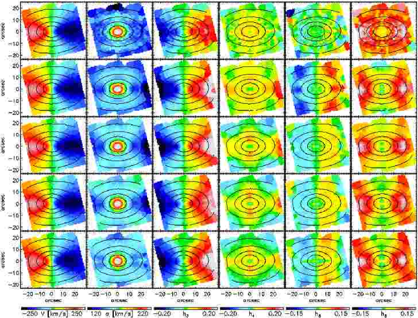
Figure 12: Comparison of the symmetrised observation of NGC 2974 (first row) and four orbital superposition models with best mass-to-light ratio $\Upsilon$, for a given inclination i. From second row to bottom: ($i,\Upsilon$) = ($55,4.4$), ($65,4.5$), ($75,4.7$), ($89,4.8$). From left to right each panel presents: mean velocity $V$, velocity dispersion $\sigma$, and Gauss-Hermite moments: $h_{3},h_{4},h_{5}$ and $h_{6}$. Isophotal contours of total light are shown with solid lines.

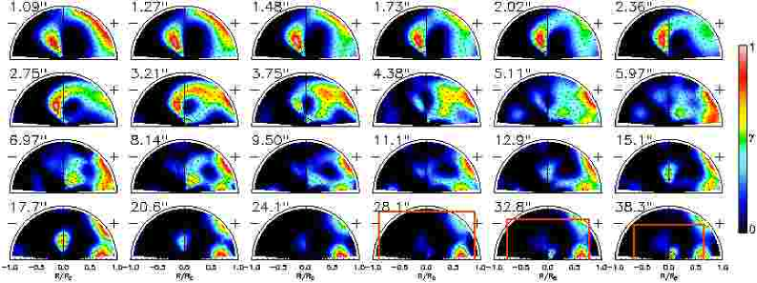
Figure 13: Integral space of the best-fitting orbit superposition model for NGC 2974. Each panel plots the meridional plane ($R$,$z$) with the starting positions of orbits (dots) for the given energy. Orbital starting positions correspond to the position of cusps ($v_{R}=v_{z}=0$). Overplotted is the fraction of mass assigned to orbits at constant energy, labelled by the radius of the circular orbit in arcseconds (printed at the upper left corner of each panel). The radius of the circular orbit is the size of the horizontal axis (measured from the centre). Negative values are obtained by sign reversal, since orbits can be prograde and retrograde. Orbits with high angular momentum are found in the right and left corner respectively on the plots. We show only the radii constrained by the data. The last three panels have the size of the SAURON  field overplotted for comparison (red rectangle). The area inside the rectangle is constrained by the kinematic data. The colour bar on the right represents the relative colour coding of the orbital mass weights ($\gamma$), where 1 represent the largest mass weight assigned to an orbit at the given energy.

A standard mathematical approach to solve inverse problems is by regularising (e.g. Press et al., 1992, Chapter 18). This has been generally applied by all groups involved in this modelling approach (e.g. Rix et al., 1997; Gebhardt et al., 2003; Valluri et al., 2004; Cretton & Emsellem, 2004). Regularisation inevitably biases the solution, by forcing most orbits to have a non-zero weight. The key here is to apply the right amount of regularisation. Previous tests with the Schwarzschild code suggested a value of the regularisation parameter $\Delta=4$ (see Cretton et al. 1999; V02). After initial testing we also adopted this value. For more details on regularisation, see McDermid et al. (in prep.).

The models are axisymmetric by construction. In order to avoid possible systematic effects we additionally symmetrise the stellar kinematics as usually done in other studies. The symmetrisation uses the mirror-(anti)-symmetry of the kinematic fields, such that kinematic values from four symmetric positions ($(x,y),(x,-y),(-x,y),(-x,-y)$) were averaged. However, the Voronoi bins have irregular shapes and they are not equally distributed with respect to the symmetry axes of the galaxy (minor and major axes). In practice, we average the four symmetric points, and, if for a given bin there are no bins on the symmetric positions, we interpolate the values on those positions and then average them. As the number of data points is not decreased in this way, the errors were left unchanged.

Finally, we fitted axisymmetric dynamical models to symmetrised observations of velocity, velocity dispersion and Gauss-Hermite moments ($h_{3}-h_{6}$) while varying the mass-to-light ratio $\Upsilon$ and the inclination $i$. Figure 11 shows a grid of our models with overplotted $\Delta\chi^{2}$ contours. The best-fit parameters are $\Upsilon=4.5\pm 0.1$ (in the $I$ band) and $i=65\degr\pm 2.5\degr$. The data – model comparison for these values is given in Fig. 12 (symmetrised data are shown in the first row and the best-fitting model in the third row). In the same figure we present the best-fitting models for the given inclinations. The formal statistical analysis firmly rules out (with $3\sigma$ confidence) all inclinations outside $i=65\degr\pm 2.5\degr$. The differences between the models are only marginally visible on Fig. 12. However, comparing the models with the top row of symmetrised data, it is noticeable that the velocity dispersion is less well fitted with increasing inclination. On the other hand, the fit to $h_{3}$ improves with higher inclinations. Higher-order moments change similarly and the final $\chi^{2}$ is the result of this combined effect. Surprisingly, the difference between the best-fit model and the data are bigger than the difference between the other models and the best-fit model, provoking a question whether the determination of the inclination is robust.

Recently, EGF03 used two-integral $f(E,L_{z})$ dynamical models and found a best fit for an inclination of 60° but also stated that models with $58\degr\leq i\leq 65\degr$ fit equally well. Our three-integral models have a larger freedom in fitting the observations and it is unknown whether these models can uniquely constrain the inclination. Our obtained inclination is close to the previous measurements in the literature (references in Sections 1 and 2), and also to the inclination measured from gas and dust. NGC 2974 is perhaps a special case (in terms of its intrinsic structure and geometry) for which three-integral models are able to give a stronger constraint on the inclination. We return to this issue in Section 5.2.

The integral space of the best-fitting model, (i.e. the space defined by the isolating integrals of motion ($E,L_{z},I_{3}$) that define the orbits and the DF $f=f(E,L_{z},I_{3})$), is shown in Fig. 13. Each panel presents mass assigned to orbits of constant energy, parameterised by the radius of the circular orbit. This orbit also has the maximum angular momentum and circular orbits of negative and positive angular momentum are in the bottom left and right corner of each plot, while the low angular momentum orbits are close to the symmetry ($y$) axis. An interesting feature dominates the panels with radii larger then 5$\aas@@fstack{\prime\prime}$11. A high fraction of mass is assigned to orbits with high angular momentum. This indicates that the bulk of the stars between these radii rotate with high angular momentum. A possible physical interpretation is that a large fraction of the stars orbit in a disc. Cinzano & van der Marel (1994) argued that NGC 2974 has an embedded stellar disc and in their two-integral Jeans models they were not able to fit the stellar kinematics without introducing a disc with $\approx 7\%$ of the total galaxy light. On the other hand, the two-integral models of EGF03 did not need to invoke an additional stellar disc component to fit data consisting of their TIGER data and the three long slits of Cinzano & van der Marel (1994). The integral space presented here suggests that the three-integral models need orbits with high angular momentum, but the selected orbits also have different values of $I_{3}$, and therefore do not represent a very thin stellar disc as assumed by Cinzano & van der Marel (1994), but a somewhat flattened distribution of stars like in a normal S0. The relative light contribution of the high-angular momentum orbits is $\approx 10\%$, which corresponds to a total stellar mass of $1.5\times 10^{10}\>{\rm M_{\odot}}$ assuming the best-fit model inclination and $\Upsilon$.

5 Tests of Schwarzschild’s orbit-superposition models

In the previous section we used three-integral models to recover the inclination, mass-to-light ratio and the internal structure of NGC 2974. Surprisingly, we find that the inclination is tightly constrained by $\chi^{2}$ contours (Fig. 11), although the difference between the models (Fig. 12) are smaller than the difference between formally the best-fitting model and the data. In this section, we wish to test the robustness of those results as well as the general ability of the three-integral models to recover the given parameters. For this purpose we constructed an axisymmetric model mimicking NGC 2974 using two integrals of motion: the energy $E$, and the $z$-component of the angular momentum, $L_{z}$. This two-integral galaxy model has the advantage of a known DF, $f=f(E,L_{z}$), everywhere, which we want to compare with the results of the three-integral modelling. There are three issues we wish to test:

• Recovery of the input parameters of the two-integral model galaxy. This is a general test to show whether the three-integral method can recover the parameters used in construction of a test model. We wish to be consistent with the observations and consider only the recovery of the input mass-to-light ratio and inclination, especially in light of the results from the Section 4.

• Influence of the spatial coverage. The SAURON kinematic observations of NGC 2974 roughly cover one effective radius. This is also the typical size of most kinematic observations of other early-type galaxies from the SAURON  sample. Here we want to test the influence of the limited extent of the kinematic coverage on the recovery of the orbital distribution. We do this by comparing the difference between models using a limited and a full spatial kinematic information provided by the two-integral galaxy model.

• The recovery of the input DF. We wish to test the ability of our three-integral models to correctly recover the true input (two-integral) DF. Similar tests were also presented by Thomas et al. (2004) for their implementation of Schwarzschild’s method. Cretton et al. (1999) and Verolme & de Zeeuw (2002) and Cretton & Emsellem (2004) described similar tests using two-integral Schwarzschild models.

5.1 The input two-integral test model

An $f(E,L_{z})$ model of NGC 2974 was constructed using the Hunter & Qian (1993) contour integration method (hereafter HQ, see also Qian et al. 1995). We used the mass model from Section 4.1 parameterised by MGE. This approach follows in detail Emsellem et al. (1999), and, due to the properties of Gaussian functions, simplifies the numerical calculations significantly. Given the density of the system, the HQ method gives the unique even part of the DF, $f_{e}=\frac{1}{2}[f(E,L_{z})+f(E,-L_{z})]$ (even in $L_{z}$). The odd part can be calculated as a product of the even $f_{e}$ and a prescribed function $h=h(L/L_{z})$. The magnitude of the function $h$ is chosen to be smaller than unity, which ensures that the final DF, $f=f_{e}+f_{o}$, is physical (i.e. non-negative, provided that $f_{e}>>0$ everywhere). In practice, the odd part is chosen to fit the observed kinematics (mean streaming) by flipping the direction of orbits with respect to the symmetry axis (photometric minor axis).

The two-integral model of NGC 2974 was computed using $i=60\degr$ and $\Upsilon=4.6$. In order to construct a realistic DF we also included a black hole with mass $M_{BH}=2.5\times 10^{8}\>{\rm M_{\odot}}$, from the $M_{\rm BH}-\sigma$ relation. The MGE model, constructed from a finite spatial resolution HST WFPC2 image, has by construction an unrealistic flat asymptotic density profile well inside the central observed pixel ($r\la 0\aas@@fstack{\prime\prime}02$) and therefore we assumed a cusp with a power-law slope of 1.5 ($\rho=r^{-1.5}$) inside that radius, following the prescription of Emsellem et al. (1999). The final two-integral DF was computed on a fine adaptive grid (i.e. more points in the region of strongly-changing DF with $E/E_{max}<2$, where $E_{max}$ is the value of the central potential of the model excluding the black hole) of $140\times 79$ points in ($E,L_{z}$). A fine grid of LOSVDs was computed from this DF. These LOSVDs were used to compute the observable LOSVDs on 3721 positions, two-dimensionally covering one quadrant of the sky plane ($50\arcsec\times 50\arcsec$), accounting for the instrumental set up (size of SAURON pixels) and atmospheric seeing (which matched the observations of NGC 2974 and was used for the three-integral models in Section 4.2). The parameters of the two-integral model of NGC 2974 are listed in the first column of Table 6.

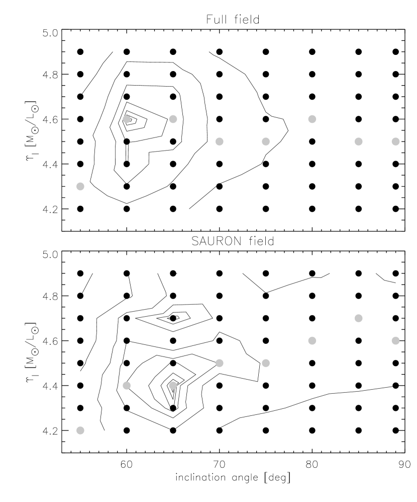
Figure 14: Three-integral model grids of inclination angle versus $M/L$ ratio, $\Upsilon$. Contours present constant $\Delta\chi^{2}$, measuring the goodness of fit of the models. Every symbol corresponds to a three-integral axisymmetric model with given inclination angle and $\Upsilon$. The grey symbols indicate the best fitting models at a given inclination. The top grid presents models using the Full field set of kinematic constraints. The global minimum is for the model with $i=60\degr$ and $\Upsilon=4.6$. The bottom panel presents models using the SAURON field set of kinematic constraints. The global minimum here is for the model with $i=65\degr$ and $\Upsilon=4.4$.

Table 6: The properties of two-integral models and comparison to three-integral best-fit results.

$$\begin{array}[]{c|ccc}\hline\cr\vskip 3.0pt plus 1.0pt minus 1.0pt\cr&$2I model$&$Full field$&${\tt SAURON} field$\\ &(1)&(2)&(3)\\ \vskip 3.0pt plus 1.0pt minus 1.0pt\cr\hline\cr\Upsilon&4.6&4.6\pm 0.1&4.4\pm 0.1\\ i&60\degr&60\degr\pm 5\degr&65\degr\pm 5\degr\\ \vskip 3.0pt plus 1.0pt minus 1.0pt\cr\hline\cr\end{array}$$

Notes – Col.(1): parameters of the two-integral model of NGC 2974; Col.(2): recovered parameters using the Full field spatial coverage ($100\arcsec\times 100\arcsec$ effectively) of kinematic constraints; Col.(3): recovered parameters using the SAURON field spatial coverage ($40\arcsec\times 40\arcsec$ effectively) of kinematic constraints.

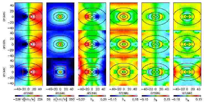
Figure 15: Comparison between two-integral analytical model kinematics and three-integral models. First row: two-integral model used as input to the three-integral code. Second row: best fitting three-integral model ($i=60\degr,\Upsilon=4.6$) using the Full field set of kinematic constraints. Third row: best-fitting three-integral model ($i=65\degr,\Upsilon=4.4$) using the SAURON field set of kinematics. The spatial extent of this set is marked by red squares on the maps. From left to right each panel presents: mean velocity $V$, velocity dispersion $\sigma$, and Gauss-Hermite moments: $h_{3},h_{4},h_{5}$ and $h_{6}$. Isophotal contours of total light are shown with solid lines.

In order to mimic the real observations (as well as to reduce the number of observables in the fit) we adaptively binned the spatial apertures using the Voronoi tessellation method of Cappellari & Copin (2003) as it was done for the observations, assuming Poissonian noise. The final LOSVDs were used to calculate the kinematic moments (V, $\sigma$, $h_{3}$ to $h_{6}$) by fitting a Gauss-Hermite series (first row on Fig. 15). These values were adopted as kinematic observables for the three-integral models. From these data we selected two sets of kinematic observables:

• The first set consisted of all 513 spatial bins provided by the two-integral model. In terms of radial coverage this Full field set extended somewhat beyond two effective radii for NGC 2974.

• The second set had a limited spatial coverage. It was limited by the extent of the SAURON observations of NGC 2974, approximately covering one effective radius. We call this observational set of 313 bins the SAURON field.

5.2 Recovery of input parameters

Our two-integral models are axisymmetric by construction and all necessary information is given in one quadrant bounded by the symmetry axes (major and minor photometric axes). Hence, the inputs to the three-integral code covered only one quadrant of the galaxy. Although only one quadrant was used for the calculations we show all maps unfolded for presentation purposes.

The three-integral models were constructed in the same way as described in Section 4.2. For both (Full field and SAURON field) sets of kinematic data we created orbit libraries of $2\times 41\times 10\times 10$ orbits and constructed models on grids of ($\Upsilon,i$). As for the real data, we used a regularisation parameter $\Delta=4$. The resulting grids are presented in Fig. 14, and the best-fitting models are listed in the Table 6. The three-integral models were able to recover the true input parameters within the estimated errors, although the SAURON field models were less accurate.

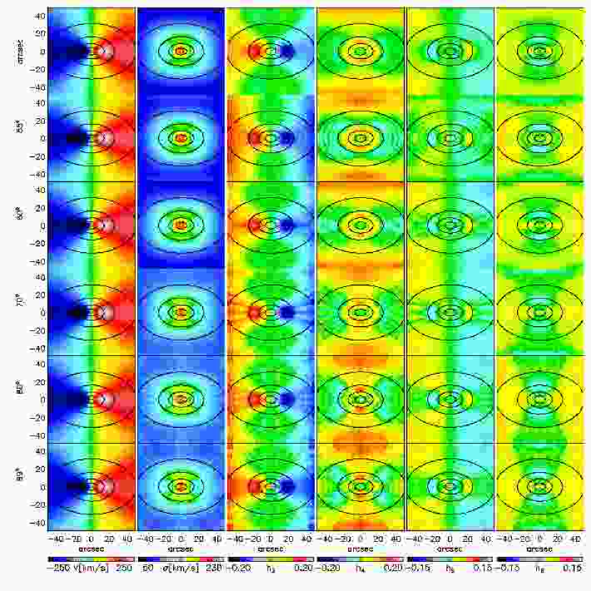
Figure 16: Sequence of three-integral models for different inclinations fitting the (Full field of kinematic observables. First row: two-integral test model. Subsequent rows: three-integral models for $i=(55\degr,60\degr,70\degr,80\degr,89\degr)$. Columns from left to right present moments of the LOSVD: $v$, $\sigma$, and from $h_{3}$ to $h_{6}$. Isophotal contours of total light are shown with solid lines.

The kinematic observables computed from the two-integral models are noiseless, without errors nor intrinsic scatter typical of real measurements. For each kinematic observable we assigned a constant error, but representative to the SAURON observations of NGC 2974: $1\sigma$ errors for $V$, $\sigma$, $h_{3}$, and $h_{4}\ldots h_{6}$ were 4$\>{\rm km}\,{\rm s}^{-1}$, 7$\>{\rm km}\,{\rm s}^{-1}$, 0.03 and 0.04 respectively.

As we wanted to test an ideal situation we computed the kinematic observables from the two-integral model without adding noise (intrinsic scatter) typical for real measurements. However, given the fact that the input model is noiseless, the $\chi^{2}$ levels computed from the fit to the kinematics are meaningless. In order to have an estimate of the uncertainties in the recovery of the parameters we computed half a dozen Monte Carlo realisations of the kinematic data, introducing the intrinsic scatter to the noiseless data. For each Monte Carlo data sets we constructed a three-integral model grid like in Fig. 14. Due to time limitations we calculated parameter grids ($\Upsilon$, $i$) of models with smaller orbit libraries ($2\times 21\times 7\times 7$ orbits) of both Full field and SAURON field data sets. In this case we also applied the regularisation scheme with $\Delta=4$. Approximate $3\sigma$ confidence levels assigned to the best-fitting parameters are listed in Table 6. Setting the regularisation to zero, we observed similar trends.

The numbers in Table 6 suggest that the inclination is formally recovered by three-integral models, as seen in the case of the observation (Section 4.3). We repeat the exercises of plotting a sequence of models with different inclinations (using the Full field kinematics). They are presented in Fig. 16 and we can see a very similar trend as in Fig. 12: there appears to be little difference between the models, although by scrutinising the details, it is possible to choose the best model by eye.

Figure 17: Comparison of the integral spaces of the $f(E,L_{z})$ test models. Upper five rows belong to the model constrained by the SAURON field kinematics and the lower five rows to the model constrained by the Full field kinematics. The meaning of each panel is the same as in Fig. 13. The colour bar on the right represents the relative colour coding of the orbital mass weights ($\gamma$), where 1 represent the largest mass weight assigned to an orbit at the given energy. In the region constrained by both kinematic sets the integral spaces are indistinguishable.

The smoothness of the data of the two-integral test model helps in recognising the best-fit model. The models with lower inclination (towards face-on) are generally smoother than the higher inclination (towards edge-on) models, which systematically show radial structures. These “rays” visible on Fig. 16 are artifacts of the discreteness of our orbit library. The starting points of the orbits correspond to the positions of orbital cusps, which carry the biggest contribution to the observables. The total number of cusps is determined by the number of orbits, and the finiteness of the orbit library is reflected in the discrete contributions of the cusps to the reconstructed observables (see Fig. 1.2 of Cappellari et al. 2004). The projection effects, however, increase the smoothness by spatially overlapping different cusps; hence, models projected at e.g. $i=60\degr$ will be smoother than models viewed edge on. We believe this effect could influence the $\chi^{2}$, favouring the lower inclination models.

Although present, this effect does not provide the only constraint on the inclination. When examined more closely, models with low inclination do reproduce certain features better, for example: the shape and amplitude of the velocity dispersion in the central 20″, $h_{3}$ and $h_{4}$ at the larger radii (towards the edge of the field), the central 10″ of $h_{5}$ and $h_{6}$. In all cases the model with $i=60\degr$ reproduces these features better than other models. Comparing the models, the most significant contribution to the $\chi^{2}$ comes from the velocity dispersion, but generally, individual observables have slightly different $\chi^{2}$ values, which increase with the inclination moving away from 60° and is visible only as a cumulative effect. This explains the similarities of the different models to the eye, although they are formally significantly different.

The difference in the model observables (which include moments up to $h_{6}$) are below the level of the expected systematics in the data (e.g. template mismatch), or in the models (e.g. regularisation or variations in the sampling of observables with orbits). In the case of NGC 2974, using high signal-to-noise two-dimensional data, the difference between the models themselves are smaller than between the best-fitting model and the data, implying that the inclination is only weakly constrained. This result suggests a fundamental degeneracy for the determination of inclination with three-integral models, which is contrary to indications from previous work by Verolme et al. (2002). Theoretical work and more general tests on other galaxies are needed for a better understanding of this issue.

5.3 Effect of the field coverage on orbital distribution

The next step is to compare in more detail the three-integral models using the two different kinematic data sets. The kinematic structures of the best-fitting models are presented in Fig. 15. In the region constrained by the kinematic data both models reproduce equally well the input kinematics. As expected the regions outside the SAURON field are not reproduced well. It is more interesting to compare the phase spaces of the models. In particular, we wish to see whether the mass weights assigned to the orbits (represented by the integrals of motion) are the same for the two models.

The corresponding integral-spaces are shown in Fig. 19. Red rectangular boxes represent the extent of the kinematics used to constrain the models. In the regions constrained by both kinematic sets, the two integral spaces are identical: both models recover the indistinguishable orbital mass weights. The differences appear at larger radii (beyond 20″), outside the area constrained by the SAURON field kinematic set. Putting this result in the perspective of observations, the resulting phase space (in the region constrained by the observations) does not depend on the extent of the radial coverage used to constrain the model. This result strengthens the case of the NGC 2974 modelling results, where we have integral-field observations reaching $\approx 1$ r_e. The recovered integral space and its features would not change significantly if we had a spatially larger observational field.

5.4 Recovery of the internal moments

We wish to see if the best-fitting three-integral model to the $f(E,L_{z})$ test galaxy model is consistent with the input, i.e., whether three-integral models will recognise the true structure of the test galaxy. A first estimate can be achieved by investigating the internal structure of the resulting model galaxy, specifically the shape of the velocity ellipsoid. We define the tangential dispersion as $\sigma_{t}=[\frac{1}{2}(\sigma^{2}_{\theta}+\sigma^{2}_{\phi})]^{1/2}$. Note that $\sigma_{\phi}$ includes only random motion so that for an isotropic distribution, under the given definition, the radial ($\sigma_{r}$) and tangential dispersion are equal. Since two-integral models are isotropic in the meridional plane per definition, we expect to recover that $\sigma_{r}$ is equal to $\sigma_{\theta}$ and the cross-term $\sigma_{R\theta}$ is equal to zero. In Fig. 18 we show the ratio of the moments of the velocity ellipsoids at different positions in the meridional plane and at different radii from the model constrained by the Full field kinematics. One can see that $\sigma_{r}=\sigma_{\theta}$ within $\approx 5\%$, confirming that our three-integral model recovers the true internal moments. Also, computing the cross-terms $\sigma_{R\theta}$, we verified that it is negligible everywhere. Similar results are also recovered from the SAURON field model: in the constrained region the ratio of $\sigma_{r}$ and $\sigma_{\theta}$ moments are consistent with unity.

Figure 18: Moments of the velocity ellipsoid for the two-integral test galaxy recovered by the three-integral model (constrained by the Full field kinematic set). The upper panel shows the ratio of the radial and tangential moment as defined in the text. The lower panel presents the ratio of the radial and latitudinal moments. Different lines show the ratio of the moments in the meridional plane at different position angles, starting from the major-axis to the minor axis. In a true two-integral galaxy, all three moments of the velocity ellipsoid have to be equal. Note that the deviation inside 1″are expected since the data do not constrain the model in that region.

5.5 Recovery of the distribution function

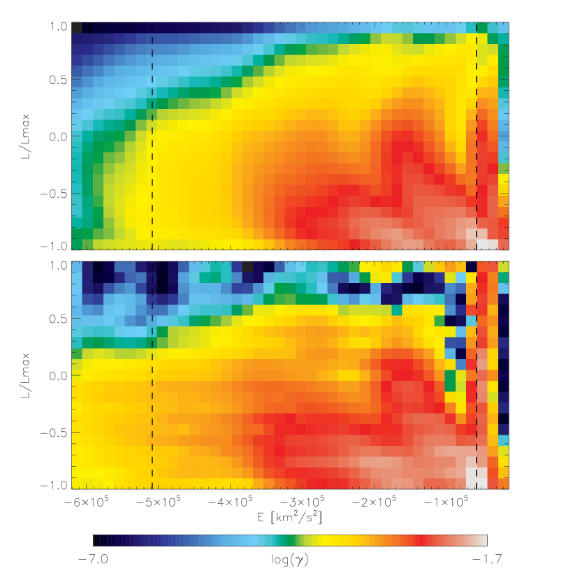
Figure 19: Comparison of the mass weights from the two-integral model (upper panel) and the results of the three-integral modelling (lower panel) using the two-integral model as input. The galaxy centre is on the left side. The first bin containing the contribution of the black hole was not plotted, since the resolution of the models do not allow for its recovery. The two vertical lines enclose the region constrained by the kinematic data. The colour bar represents the colour coding of the orbital mass weights ($\gamma$) in log scale assigned to any interval of ($E,L_{z}$). There are two main differences between the input and the best fit model: (i) the horizontal stripes, which are due to the discrete way in which we select orbits in $L_{z}$ range, and (ii) the mass weights at high $L_{z}$ values, which, however, contain a very small fraction of the galaxy mass and are not significant.

The previous result shows that the constructed three-integral model is a consistent representation of the input $f(E,L_{z})$ model. A more conclusive test, however, is to compare the distribution functions.

The results of the three-integral Schwarzschild method are orbital mass weights, $\gamma^{\prime}_{3I}(E,L_{z},I_{3})$, for each set of integrals of motion ($E$, $L_{z}$, $I_{3}$), which define an orbit. The DF is related to the mass weights via the phase-space volume (for a detailed treatment see Vandervoort 1984):

$$\gamma(E,L_{z},I_{3})\;\mathrm{d}E\mathrm{d}L_{z}\mathrm{d}I_{3}={}$$ (6)

$$f(E,L_{z},I_{3})\;\Delta V(E,L_{z},I_{3})\;\mathrm{d}E\mathrm{d}L_{z}\mathrm{d}I_{3},$$

where

$$\Delta V(E,L_{z},I_{3})=\int\limits_{\Omega}\mathcal{J}(\vec{x},E,L_{z},I_{3})\mathrm{d}^{3}x,$$ (7)

and $\mathcal{J}(\vec{x},E,L_{z},I_{3})$ is the Jacobian of the coordinate transformation from $(\vec{x},\vec{v})$ to $(\vec{x},E,L_{z},I_{3})$, and $\Omega$ is the configuration space accessible to an orbit defined by the integrals ($E$, $L_{z}$, $I_{3}$). Unfortunately, $I_{3}$ is not known analytically, so the above relation can not be explicitly evaluated, except for separable models. For this reason we limit ourselves to test the consistency of our three-integral mass weights with the input two-integral DF. This is possible, since if the recovered three-integral DF is equal to the input DF, then the mass $\gamma_{2I}(E,L_{z})$ assigned to the stars in a given range of $(E,L_{z})$ by the three-integral model has to be equal to the mass in the same range of the input model.

There exists a precise relation between the input two-integral DF, $f=f(E,L_{z})$, and the corresponding orbital mass weights, $\gamma_{2I}(E,L{z})$. The total mass of the system is the integral of the DF over the phase-space. Using this, Cretton et al. (1999) derived the expression for the mass weights in Appendix B of their paper (eq. B4):

$$\gamma_{2I}(E,L_{z})=\int\limits_{\Omega}\frac{\mathrm{d}M}{\mathrm{d}E\mathrm{d}L_{z}}\mathrm{d}E\mathrm{d}L_{z}\\$$ (8)

with

$$\frac{\mathrm{d}M}{\mathrm{d}E\mathrm{d}L_{z}}=f(E,L_{z})\times\oint\limits_{ZVC(E,L_{z})}(R\mathrm{d}z-z\mathrm{d}R)$$ (9)

where the contour integral yields the area of the zero velocity curve (ZVC). Before applying eqs. (8) and (9) on the two-integral DF we rebinned it to the same grid of $\Delta E$ and $\Delta L_{z}$ as the three-integral mass weights. Finally, we approximate the integral (8) by multiplying the mass fraction in each grid cell by $\Delta E\Delta L_{z}$.

For our comparison we defined as the energy intervals the set of energies used in the construction of the three-integral models (total of 41). The interval in angular momentum was defined as a step of 0.1 of $L_{z}/L^{max}_{z}$ from $-1$ to $+1$ (total of 20) for a given energy. The resulting grid of orbital weights is relatively coarse, but is representative of the model. The agreement between the two sets of mass weights is shown in Fig. 19. The main features of the given two-integral test model are well reproduced by the three-integral model. Again, the mass weights should be compared in the region constrained by the data (between the vertical lines in the figure). In order to quantify the agreement we restricted the comparison to the part of the distribution of mass weights contributing significantly to the model inside this region, roughly bounded by the green levels on Fig. 19. This selected region contains about 97% of mass. The mean absolute deviation between the two sets of mass weights is 6%, with peaks around 15%, except for a narrow region towards the edge of the kinematic coverage around $E=-8\times 10^{4}km^{2}s^{-2}$ and with $L_{z}/L^{max}_{Lz}>0$, where deviations can reach 35%. The mass weights of the three-integral model are also relatively noisy which is mostly the consequence of imposed discreteness as well as the numerical nature of the method.

From our test model, where the potential is known, we conclude that the Schwarzschild method can reliably recover the input distribution function within the region constrained by two-dimensional kinematics (including higher-order moments). We have already shown that the existence of constraints outside of an effective radius does not significantly affect the orbital distribution inside an effective radius. This suggests that, in the region constrained by integral-field kinematics, a representative DF can be recovered using the Schwarzschild method.

6 Modelling of emission-line gas

Clearly, with its prominent gas component, NGC 2974 is an unusual elliptical galaxy. The observations indicate the morphological similarity between the small (HII) and large scale (HI) gas discs. Also, long-slit measurements of stellar and gas motions detect similarities between the stellar and gas kinematics (Kim, 1989; Cinzano & van der Marel, 1994). In this section we investigate the inclination of the gaseous component as well as construct dynamical Jeans model of the gas disc as is Cinzano & van der Marel (1994), in order to compare them to the results of the stellar dynamical modelling.

6.1 Inclination of the gas disc

The existence of the emission-line gas disc in NGC 2974 can be used to infer the inclination of the galaxy assuming an equilibrium dynamical configuration. This has been attempted before and in all studies the inclination of the gas disc was consistent with $55\degr-60\degr$ (Amico et al. 1993 55°; Buson et al. 1993 59°; CvdM94 57.5°; Plana et al. 1998 60°). The high quality of the two-dimensional SAURON kinematics allows us to estimate the inclination of the emission-line gas disc more accurately.

Figure 20: $\Delta\chi^{2}$ as a function of inclination obtained by comparing the symmetrised data for NGC 2974 and the model gas disc velocity map described in 6.1.

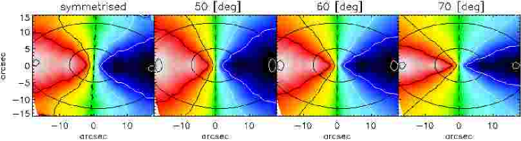
Figure 21: Comparisons between observed and model gas disc velocity fields. From left to right: observations (symmetrised), model fields for inclinations of 50$\degr$, 60$\degr$ (best-fitting), 70$\degr$. Isophotal contours of total light are presented with ellipses.

We assume the motion of the emission-line gas is confined to a thin axisymmetric disc. We neglect the deviations from axisymmetry discussed in Section 3, and symmetrise the gas velocity map in the same way as the stellar velocity map in Section 4.3. This velocity map is an axisymmetric representation of the observed field, which can be compared to an axisymmetric model of the disc velocity maps. Constructing a model axisymmetric two-dimensional velocity map requires only the kinematic major axis velocity profile $v^{\prime}_{mj}$. The entire map is then given by the standard projection formula:

$$v_{LOS}(x^{\prime},y^{\prime})=v_{\phi}\Big{(}\frac{x^{\prime}\sin i}{r}\Big{)}=v^{\prime}_{mj}\Big{(}\frac{x^{\prime}}{r}\Big{)},$$ (10)

where $r^{2}=x^{\prime 2}+(y^{\prime}/\cos i)^{2}$ and $i$ is the inclination of the disc. It is clear from this formula that for a given observed major-axis velocity, the velocity field is just a function of inclination. From the first three odd coefficients ($c_{1}$, $c_{3}$ and $c_{5}$) of the kinemetric expansion we construct the velocity profile $v^{\prime}_{mj}$ along the major axis ($\theta$ = $\overline{\phi_{1}}$). Using the major axis velocity profile, we created a set of disc velocity fields inclined at different values of $i$, and compared them with the symmetrised velocity field. We did not correct for the influence of the PSF as this effect is small and is confined to the central few arcseconds, which we excluded from the comparison. We also compared the models with the non-symmetrised velocity map and the results were in very good agreement, but with a slightly larger uncertainty range.

Figure 20 presents the $\Delta\chi^{2}$ obtained by subtracting the disc model velocity field from the symmetrised measurements. The best-fitting inclination is $i=60\degr\pm 3\degr$ (at $1\sigma$ level). Fig. 21 shows a comparison between the symmetrised and model velocity fields for a few representative inclinations. The differences between the model fields are mostly in the opening angle of the iso-velocity contours, which change with the inclination of the field. The opening angle of the model with $i=60\degr$ is the most similar the observed velocity field and this significantly lowers the $\chi^{2}$ of the fit.

The best-fit inclination of $60\degr$ for the emission-line gas is in excellent agreement with literature values determined from the various gas components. Our best-fitting three-integral stellar dynamical model was obtained for an inclination of $65\degr$ with $3\sigma$ uncertainty of $2.5\degr$. This inclination is close to the inclination of $60\degr$ presented in this section, suggesting a good agreement between the stellar and gaseous models. There is, however, the concern that the agreement may not be as significant as it seems in light of the tests and results from Section 5.2.

6.2 A simple dynamical model for the disc

At large scale, the gas kinematic maps are consistent with the assumption that the emission-line gas is moving in a thin disc. This assumption clearly breaks down in the inner few arcseconds, but at this point we neglect this effect. The observed gas velocity dispersion is high everywhere in the disc and is much larger than the thermal velocity dispersion which should be of the order of $\sigma_{thermal}\sim 10\>{\rm km}\,{\rm s}^{-1}$ (Osterbrock, 1989) and in any case $<30\>{\rm km}\,{\rm s}^{-1}$. Clearly, in addition to the thermal dispersion, the gas has another source of motion, which is not presently understood, but is seen in many galaxies (Bertola et al., 1995). Several studies (e.g. van der Marel & van den Bosch, 1998; Verdoes Kleijn et al., 2000) assumed that the non-thermal gas velocity dispersion is the result of ‘local turbulence’, without describing the details of the underlying physical processes. In this assumption, the gas still rotates at the circular velocity and the invoked turbulence does not disturb the bulk flow of the gas on circular orbits. The alternative to this assumption is that the non-thermal velocity dispersion component comes from collisionless gravitational motion of the gas, where the gas acts like stars: clumps of gas move on self-intersecting orbits. This is, perhaps, not very physical for gas in general, but it can be applied to estimate the difference between the circular and streaming velocity (and including the projection effect on the observed velocity) of the gas. Several studies used this approach successfully (e.g. Cinzano & van der Marel, 1994; Cretton et al., 2000; Barth et al., 2001; Aguerri et al., 2003; Debattista & Williams, 2004). Presently, the role and importance of the asymmetric drift remains an unresolved issue.

Figure 22: Fit to the surface-density profile of the [OIII] emission lines. Dashed lines present individual exponentials given by eq.(12).

Figure 23: Ratio $\sigma_{R}/V_{C}$ for the best-fitting model to the emission-line gas data.

In constructing our simple disc model we assumed that the emission-line gas is moving in individual clumps that interact only collisionlessly. The clumps move along ballistic trajectories in a thin disc, under the influence of the galaxy potential given by the stellar distribution (Section 4). The gas kinematics are determined by solving the Jeans equations for radial hydrostatic equilibrium. Following Binney & Tremaine (1987, eq. 4-33), the streaming velocity of gas can be written in cylindrical coordinates as:

$$\bar{v}_{\phi}^{2}=V_{c}^{2}-\sigma_{R}^{2}\Big{[}-R\frac{\mathrm{d}\ln\rho}{\mathrm{d}R}-R\frac{\mathrm{d}\ln\sigma_{R}^{2}}{\mathrm{d}R}-(1-\frac{\sigma_{\phi}^{2}}{\sigma_{R}^{2}})\Big{]}$$ (11)

where we have assumed the distribution function depends on the two classical integrals of motion, $f=f(E,L_{z})$, which implies $\sigma_{R}$ = $\sigma_{z}$ and $\overline{v_{R}v_{z}}$ = 0. In eq. (11), V_c is the circular velocity ($\sqrt{R(\mathrm{d}\Phi/\mathrm{d}R)}$), $\Phi$ is the total potential of the galaxy obtained from the MGE fit assuming inclination $i$, $\sigma_{R}$ and $\sigma_{\phi}$ are the radial and azimuthal velocity dispersions, and $\rho$(R) is the spatial number density of gas clouds in the disc. Lacking any alternative, we use the surface brightness of the gas to estimate $\rho$(R). Instead of using the actual measured values of the [OIII] and H$\beta$ flux, we parametrise the emission-line surface brightness with a double exponential law,

$$\rho=\rho_{0}e^{-\frac{R}{R_{0}}}+\rho_{1}e^{-\frac{R}{R_{1}}},$$ (12)

in order to decrease the noise. The parameters are obtained from the fit to the [OIII] data shown in (Fig. 22), where the two-dimensional surface brightness was collapsed to a profile by averaging along ellipses of constant ellipticity (ellipticity of the galaxy) and position angle (PA of the galaxy). The errors are standard deviations of the measurements along each ellipse.

The relation between radial and azimuthal velocity dispersions can be obtained using the epicyclic approximation. This gives (following eq. 4-52 in Binney & Tremaine 1987):

$$\frac{\sigma_{\phi}^{2}}{\sigma_{R}^{2}}=\frac{1}{2}\Big{(}1+\frac{\mathrm{d}\ln V_{c}}{\mathrm{d}\ln R}\Big{)}$$ (13)

This approximation is valid for small values of the asymmetric drift $v_{\phi}-V_{c}$, or, in other words, in the limit of a cold disc with small velocity dispersion, $\sigma\ll V_{c}$. This is marginally the case in NGC 2974, clearly violated in the central $<5\arcsec$, but it is acceptable in most of the observed regions (Fig. 23).

The observed quantities can be obtained from the calculated intrinsic properties projecting at an inclination angle $i$. The projected two-dimensional line-of-sight (LOS) velocity field is given by eq. (10). Within these assumptions of the disc model, the projected LOS velocity dispersion is:

$$\sigma^{2}_{LOS}=(\sigma_{\phi}^{2}-\sigma_{R}^{2})\Big{(}\frac{x^{\prime}\sin i}{r}\Big{)}^{2}+\sigma_{R}^{2}$$ (14)

We constructed the asymmetric drift models of the emission-line gas in NGC 2974 using the MGE parametrisation of the potential, $\Upsilon$=4.5, inclination $i=60\degr$, and simultaneously accounting for the atmospheric seeing and pixel size of the SAURON observations (see Qian et al. 1995 for details). In the process we assumed an exponential law for the radial velocity dispersion:

$$\sigma_{R}=\sigma_{0}+\sigma_{1}e^{-\frac{R}{R_{\sigma}}},$$ (15)

Our models, therefore, have three free parameters, $\sigma_{0}$, $\sigma_{1}$, and $R_{\sigma}$, and varying them we constructed gaseous disc models of NGC 2974. The models were compared with the symmetrised velocity and velocity dispersion maps averaging the four symmetric positions on the maps as required for an axisymmetric map (Section 4.3). The best-fitting model was obtained for $\sigma_{0}=85\pm 5\>{\rm km}\,{\rm s}^{-1}$, $\sigma_{1}=180\pm 10\>{\rm km}\,{\rm s}^{-1}$, and $R_{\sigma}=5\pm 1\arcsec$. Comparison of this model with the symmetrised observations is presented in Fig.  24.

This simple asymmetric drift model can reproduce rather well the general properties of the emission-line gas disc, including the bulk of the streaming velocity as well as the significant non-zero velocity dispersion. The overall fit is quite good with a mean difference of only 5%, with peaks up to about 20%. The main discrepancy occurs along the major-axis at a radius around 10″, close to where we observe the presumed elliptical ring in the ionised gas equivalent width (see Fig. 6). The observed minor-axis elongation of the gas velocity dispersion is also not reproduced by the model. This is not surprising since some of those features, as mentioned, are signatures of non-axisymmetry in NGC 2974, and cannot be represented by simple axisymmetric models.

Since the normalisation of the kinematics is mostly controlled by the assumed mass-to-light ratio, the goodness of the fit implies that the overall energy budget coming from the Schwarzschild modelling is consistent with the observed gas kinematics: the high value of the gas velocity dispersion is therefore globally compensated by a lower mean velocity. A similar finding was reported by Cinzano & van der Marel (1994). All this therefore raises the question of how the gas can remain dynamically hot in a disc galaxy like NGC 2974 at a scale of $\sim 1$ kpc.

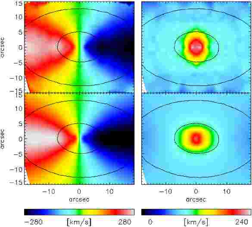
Figure 24: Bottom Panels: Asymmetric drift model for the best fitting parameters compared to Top Panels: the symmetrised (mirror-(anti)-symmetric filtering with 6 terms) mean velocity (first column) and velocity dispersion (second column). Overplotted isophotes are levels of the reconstructed total intensity.

7 Concluding remarks

This paper presents a case study of the early-type galaxy NGC 2974, which was observed in the course of the SAURON survey of nearby E/S0 galaxies.

Kinematic position angles of the stellar and gaseous kinematics of this galaxy are on average well aligned. The stellar kinematic maps exhibit point- and mirror-(anti)-symmetry, with the kinematic angle equal to the photometric PA, and are consistent with an axisymmetric intrinsic shape. The gaseous velocity map is more complicated, with clear departures from axisymmetry in the centre of the galaxy ($<4\arcsec$). At larger radii, the gas kinematic angle is not constant, although is largely consistent with the photometric PA, showing deviations of a few degrees. The SAURON observations of NGC 2974 confirm the existence of non-axisymmetric perturbations consistent with an inner bar (EGF03) as well as a possible large-scale bar. The departures from axisymmetry are not visible in the stellar kinematic maps and therefore are likely to be weak. This allows us to construct axisymmetric models of NGC 2974.

We constructed self-consistent three-integral axisymmetric models based on the Schwarzschild’s orbit superposition method, varying mass-to-light ratio and inclination. The observed surface brightness was parameterised by multi-Gaussian expansion model on both ground- and space-based imaging. The models were compared with the SAURON kinematic maps of the first six moments of the LOSVD ($v$, $\sigma$, $h_{3}$ - $h_{6}$). The best-fitting model has $\Upsilon=4.5\pm 0.1$ and $i=65\degr\pm 2.5\degr$. The inclination is formally well constrained, but there are several indications that the recovery of the inclination is uncertain: (i) differences between the models are on the level of the expected systematics in the data (e.g. template mismatch); (ii) difference between the best-fit model and the data are bigger than differences between other models and the best-fit model; (iii) limitations of the models (discreteness of the cusps) may artificially constrain the inclination.

The internal structure of NGC 2974 (assuming axisymmetry) reveals the existence of a rapidly rotating component contributing with about 10% of the total light. This component is composed of orbits allowing the third integral and does not represent a cold stellar disc, although suggests a flattened structure similar to an S0 galaxy.

The results of the stellar dynamical models were compared with the results of modelling the gas component. The inclination of the gas disc, calculated from the emission-line velocity map is $i=60\degr\pm 3$, in agreement with the formally constrained stellar inclination. A simple model of the gas disc in the same potential used for the stellar modelling ($\Upsilon=4.5$, but $i=60\degr$) was able to reproduce the characteristics of the gas kinematics ($v$ and $\sigma$) on the large scale, but, as expected, failed in the centre. In general, the observed gas kinematics is consistent with being produced by gravitational potential determined by the stellar dynamical models, but the origin of the high velocity dispersion of the gas on large scales remains an open question.

We performed a set of tests of our implementation of the Schwarzschild’s orbit superposition method. For this purpose we constructed a general two-integral model of NGC 2974, and used the reconstructed kinematics as inputs to the Schwarzschild’s method. We tested (i) the influence of the radial coverage of the kinematic data on the internal structure, (ii) the recovery of the test model parameters ($\Upsilon$,$i$), and (iii) the recovery of the test model DF. The tests show that:

1. Increasing the radial coverage of the kinematic data from $1r_{e}$ to $2r_{e}$ does not change the internal structure within $1r_{e}$. The results of the dynamical models of the SAURON observations of NGC 2974 would not change if the radial coverage would be increased by a factor of 2.

2. We find that three-integral models can accurately recover the mass-to-light ratio. Although the models are also able to constrain the inclination of the test model formally, the apparent differences between the models are small (as in the case of the real observations). Under careful examination, it is possible to choose the best model by eye, but the decisive kinematic features are below (or at the level) of the expected systematics in the data (e.g. template mismatch) and might be influenced by the uncertainties in the models (e.g. regularisation or variations in the sampling of observables with orbits). This suggest a degeneracy of models with respect to the recovery of inclination. More general tests on other galaxies and theoretical work is needed for a better understanding of this issue.

3. From a realistic test model, the analytically known input DF is recovered within 6% in the region constrained by integral-field kinematics. This suggests that applying the Schwarzschild technique with integral-field kinematics can reliably recover a representative DF.

Acknowledgements

We thank Glenn van de Ven for fruitful discussions about the recovery of the DF. DK was supported by NOVA, the Netherlands Research school for Astronomy. MC acknowledges support from a VENI grant award by the Netherlands Organization of Scientific Research (NWO).

References

- Aguerri et al. (2003) Aguerri J. A. L., Debattista V. P., Corsini E. M., 2003, MNRAS, 338, 465
- Amico et al. (1993) Amico P., et al., 1993, in Danziger I, J., Zellinger W. W., Kjaerp K., eds, Structure, Dynamics and Chemical Evolution of Elliptical Galaxies. ESO, Garching, p. 225
- Bacon et al. (2001) Bacon R., et al., 2001, MNRAS, 326, 23
- Barth et al. (2001) Barth A. J., Sarzi M., Rix H., Ho L. C., Filippenko A. V., Sargent W. L. W., 2001, ApJ, 555, 685
- Bender (1988) Bender R., 1988, A&A, 193, L7
- Bertola et al. (1995) Bertola F., Cinzano P., Corsini E. M., Rix H., Zeilinger W. W., 1995, ApJ, 448, L13+
- Binney & Tremaine (1987) Binney J., Tremaine S., 1987, Galactic dynamics. Princeton, NJ, Princeton University Press, 1987, 747 p.
- Bregman et al. (1992) Bregman J. N., Hogg D. E., Roberts M. S., 1992, ApJ, 387, 484
- Buson et al. (1993) Buson L. M., et al., 1993, A&A, 280, 409
- Cappellari (2002) Cappellari M., 2002, MNRAS, 333, 400
- Cappellari & Copin (2003) Cappellari M., Copin Y., 2003, MNRAS, 342, 345
- Cappellari & Emsellem (2004) Cappellari M., Emsellem E., 2004, PASP, 116, 138
- Cappellari et al. (2002) Cappellari M., Verolme E. K., van der Marel R. P., Kleijn G. A. V., Illingworth G. D., Franx M., Carollo C. M., de Zeeuw P. T., 2002, ApJ, 578, 787
-
Cappellari et al. (2004)
Cappellari M.,
et al., 2004, in Ho L. C., ed, Carnegie Observatories Astrophysics
Series, Vol. 1: Coevolution of Black Holes and Galaxies, (Pasadena:
Carnegie Observatories;
http://www.ociw.edu/ociw/symposia/series/
symposium1/proceedings.html) - Cinzano & van der Marel (1994) Cinzano P., van der Marel R. P., 1994, MNRAS, 270, 325
- Copin et al. (2001) Copin Y., et al., 2001, in SF2A-2001: Semaine de l’Astrophysique Francaise Kinemetry: quantifying kinematic maps. p. 289
- Copin et al. (2004) Copin Y., Cretton N., Emsellem E., 2004, A&A, 415, 889
- Cretton et al. (1999) Cretton N., de Zeeuw P. T., van der Marel R. P., Rix H., 1999, ApJS, 124, 383
- Cretton & Emsellem (2004) Cretton N., Emsellem E., 2004, MNRAS, 347, L31
- Cretton et al. (2000) Cretton N., Rix H., de Zeeuw P. T., 2000, ApJ, 536, 319
- Cretton & van den Bosch (1999) Cretton N., van den Bosch F. C., 1999, ApJ, 514, 704
- de Zeeuw et al. (2002) de Zeeuw P. T., et al., 2002, MNRAS, 329, 513
- Debattista & Williams (2004) Debattista V. P., Williams T. B., 2004, ApJ, 605, 714
- Emsellem et al. (2004) Emsellem E., et al., 2004, MNRAS, 352, 721
- Emsellem et al. (1999) Emsellem E., Dejonghe H., Bacon R., 1999, MNRAS, 303, 495
- Emsellem et al. (2003) Emsellem E., Goudfrooij P., Ferruit P., 2003, MNRAS, 345, 1297
- Emsellem et al. (1994) Emsellem E., Monnet G., Bacon R., 1994, A&A, 285, 723
- Erwin & Sparke (2002) Erwin P., Sparke L. S., 2002, AJ, 124, 65
- Erwin & Sparke (2003) Erwin P., Sparke L. S., 2003, ApJS, 146, 299
- Franx et al. (1994) Franx M., van Gorkom J. H., de Zeeuw T., 1994, ApJ, 436, 642
- Friedli & Martinet (1993) Friedli D., Martinet L., 1993, A&A, 277, 27
- Gebhardt et al. (2003) Gebhardt K., et al., 2003, ApJ, 583, 92
- Gerhard (1993) Gerhard O. E., 1993, MNRAS, 265, 213
- Goudfrooij et al. (1994) Goudfrooij P., Hansen L., Jorgensen H. E., Norgaard-Nielsen H. U., de Jong T., van den Hoek L. B., 1994, A&AS, 104, 179
- Hunter & Qian (1993) Hunter C., Qian E., 1993, MNRAS, 262, 401
- Kim (1989) Kim D., 1989, ApJ, 346, 653
- Kim et al. (1988) Kim D.-W., Jura M., Guhathakurta P., Knapp G. R., van Gorkom J. H., 1988, ApJ, 330, 684
- Laine et al. (2002) Laine, S., Shlosman, I., Knapen, J. H., & Peletier, R. F. 2002, ApJ, 567, 97
- Lawson & Hanson (1974) Lawson C. L., Hanson R. J., 1974, Solving least squares problems. Prentice-Hall Series in Automatic Computation, Prentice-Hall, Englewood Cliffs
- Osterbrock (1989) Osterbrock D. E., 1989, Astrophysics of gaseous nebulae and active galactic nuclei., University Science Books, Sausalito, CA
- Pfenniger & Norman (1990) Pfenniger D., Norman C., 1990, ApJ, 363, 391
- Plana et al. (1998) Plana H., Boulesteix J., Amram P., Carignan C., Mendes de Oliveira C., 1998, A&AS, 128, 75
- Press et al. (1992) Press W. H., Teukolsky S. A., Vetterling W. T., & Flannery B. P., 1992, Numerical Recipes in FORTRAN 77. 2d ed, Cambridge Univ. Press, Cambridge
- Qian et al. (1995) Qian E. E., de Zeeuw P. T., van der Marel R. P., Hunter C., 1995, MNRAS, 274, 602
- Rix et al. (1997) Rix H., de Zeeuw P. T., Cretton N., van der Marel R. P., Carollo C. M., 1997, ApJ, 488, 702
- Rix & White (1992) Rix H., White S. D. M., 1992, MNRAS, 254, 389
- Rybicki (1987) Rybicki G. B., 1987, in de Zeeuw P. T., ed, IAU Symp. 127: Structure and Dynamics of Elliptical Galaxies, p 397, Reidel, Dordrecht
- Schoenmakers et al. (1997) Schoenmakers R. H. M., Franx M., de Zeeuw P. T., 1997, MNRAS, 292, 349
- Schwarzschild (1979) Schwarzschild M., 1979, ApJ, 232, 236
- Schwarzschild (1982) Schwarzschild M., 1982, ApJ, 263, 599
- Thomas et al. (2004) Thomas, J., Saglia, R. P., Bender, R., Thomas, D., Gebhardt, K., Magorrian, J., Richstone, D., 2004, MNRAS, 353, 391
- Tonry et al. (2001) Tonry J. L., Dressler A., Blakeslee J. P., Ajhar E. A., Fletcher A. B., Luppino G. A., Metzger M. R., Moore C. B., 2001, ApJ, 546, 681
- Tremaine et al. (2002) Tremaine S., et al., 2002, ApJ, 574, 740
- Valluri et al. (2004) Valluri M., Merritt D., Emsellem E., 2004, ApJ, 602, 66
- van der Marel et al. (1998) van der Marel R. P., Cretton N., de Zeeuw P. T., Rix H., 1998, ApJ, 493, 613
- van der Marel & Franx (1993) van der Marel R. P., Franx M., 1993, ApJ, 407, 525
- van der Marel & van den Bosch (1998) van der Marel R. P., van den Bosch F. C., 1998, AJ, 116, 2220
- Vandervoort (1984) Vandervoort P. O., 1984, ApJ, 287, 475
- Verdoes Kleijn et al. (2000) Verdoes Kleijn G. A., van der Marel R. P., Carollo C. M., de Zeeuw P. T., 2000, AJ, 120, 1221
- Verolme & de Zeeuw (2002) Verolme E. K., de Zeeuw P. T., 2002, MNRAS, 331, 959
- Verolme et al. (2002) Verolme E. K., et al., 2002, MNRAS, 335, 517
- Wong et al. (2004) Wong T., Blitz L., Bosma A., 2004, ApJ, 605, 183