Safety in numbers: Gravitational Lensing Degradation
of the Luminosity Distance-Redshift Relation

Abstract

Observation of the expansion history of the Universe allows exploration of the physical properties and energy density of the Universe’s various constituents. Standardizable candles such as Type Ia supernovae remain one of the most promising and robust tools in this endeavor, by allowing for a direct measure of the luminosity distance-redshift curve, and thereby producing detailed studies of the dark energy responsible for the Universe’s currently accelerating expansion. As such observations are pushed to higher redshifts, the observed flux is increasingly affected by gravitational lensing magnification due to intervening structure along the line-of-sight. We simulate and analyze the non-Gaussian probability distribution function of de/amplification due to lensing of standard candles, quantify the effect of a convolution over many independent sources (which acts to restore the intrinsic average (unlensed) luminosity due to flux conservation), and compute the additional uncertainty due to lensing on derived cosmological parameters. For example, the “degradation factor” due to lensing is a factor of three reduction in the effective number of usable supernovae at $z=1.5$ (for sources with intrinsic flux dispersion of 10%). We also derive a useful expression for the effective increased dispersion in standard candles due to lensing, as a function of redshift.

1. Introduction

The next generation of cosmological probes will explore properties of our Universe with unprecedented precision. The broad aim is to characterize the global nature of the cosmology through a mapping of the expansion history of the Universe, $a(t)$. This history is fully encapsulated in the luminosity distance-redshift relation, which depends on global quantities such as the dimensionless dark matter density, $\Omega_{m}$, dark energy density, $\Omega_{w}$, and parameters describing the precise nature of the dark energy (e.g. its equation of state). Measurements of the expansion history thus enable determinations of these cosmological parameters, and in particular shed light on the nature of the dark energy.

Type Ia supernovae (SNe) are an essential tool in the direct mapping of the subtle changes in the distance-redshift relation due to the dark energy. Indeed, observations of supernovae play a major role in our confidence that the current expansion of the Universe is accelerating (Riess et al., 1998; Perlmutter et al., 1999; Tonry et al., 2003; Knop et al., 2003; Riess et al., 2004). These (calibratable) standard candles (Phillips, 1993; Riess, Press, & Kirshner, 1995; Wang et al., 2003) give a particularly direct and simple translation from observable to expansion history: the redshift of a SN is a direct measure of the expansion factor $a$ at emission, while the flux (or magnitude) of the SN relates to its distance through a cosmological inverse square law, and hence to the lookback time $t$ to the SN explosion. Thus an observation of a SN is very close to pure cosmography: drawing a map of the geometry of spacetime.

We have strong indications from cosmic microwave background radiation measurements (in concert with large-scale structure measurements) that the geometry of space is flat (Spergel et al., 2003), corresponding to a critical density Universe with total dimensionless energy density $\Omega=1$. This global statement breaks down on scales small compared with the cosmic (Hubble) scale, where a wealth of structure, from galaxies to clusters of galaxies, is apparent (and holds encoded within it a separate brand of cosmological information).

Large-scale structure also affects our goal of mapping the full spacetime geometry, representing the expansion history of the Universe. This structure, through its gravitational potential, alters the propagation of light from distant sources, including standard candles, changing the received flux and hence compromising our measures of distance. Since structure on various scales fills the Universe, every light ray is affected at some level by this gravitational lensing. However, since photons are conserved by this lensing, the mean flux over the sources is preserved. Gravitational lensing therefore adds a statistical noise to the cosmographic mapping, one that can be overcome by averaging over sufficient numbers of distant sources.

In §2 we discuss the properties of the lensing flux magnification distribution, and in §3 we show how this affects the distance-redshift relation. We carry this through in §4 to the influence on extraction of cosmological parameters, yielding both a degradation in precision and a bias, and derive a prescription for the number of standard candles as a function of redshift required to provide averaging adequate to dilute the lensing degradation below a desired level. The conclusion in §5 summarizes the circumstances in which lensing has a significant impact on cosmological parameter determination. The Appendices discuss the non-Gaussian effects of translating between flux and magnitude measurements, and the influence of compact object lensing in a “clumpy Universe” picture.

2. Lensing magnification distributions

Consider a large number of perfect standard candles (sources with identical luminosities), distributed randomly on the sky at the same high redshift $z$. When observed in an inhomogeneous Universe, they will possess a distribution of apparent luminosities, or magnitudes, due to alteration of the light ray bundle—gravitational lensing—by intervening structures along the various lines-of-sight. The form of these lensing amplification probability distribution functions (PDFs) depends both upon the underlying cosmology ($\Omega_{m}$, $\Omega_{w}$, dark energy equation of state ratio $w(z)$, etc.) and upon the nature of the structures causing the lensing (parametrized by cosmological quantities such as the mass clustering amplitude $\sigma_{8}$, as well as details of the matter distributions: the mass function of galaxies, specific density profiles of galaxies and clusters, etc.).

To determine the lensing amplification PDF we utilize the Stochastic Universe Method (SUM) presented in Holz & Wald (1998). This method is based upon a careful analysis of the assumptions needed for a physically reasonable model of a globally Robertson-Walker, but locally inhomogeneous, Universe. It calculates statistics for the full (weak and strong) lensing probability distribution of the observed image brightnesses of standard candle sources at any redshift, for a variety of cosmological models and a variety of mass distributions. It does this in a Monte Carlo fashion, randomly generating a portion of a Universe near a given photon line-of-sight, and calculating the lensing effects in this corner of the Universe. Repeating this many times, the full lensing distributions can be well approximated.

Comparisons of SUM to conventional N-body approaches can be found in Wang, Holz, & Munshi (2002), which also argues that the lensing probability distributions have a universal form. This implies that fine details of the distributions (e.g., those dependent upon unknown aspects of the matter profiles of the lenses) will have an inconsequential effect on broad characteristics of the PDFs, such as the variance, or the shift of the mode. As the current analysis is dominated by these broad features, fine details of the distributions will have little impact on our results. We use the SUM approach, rather than the universal (weak lensing) form presented in Wang, Holz, & Munshi (2002), to ensure that any effects due to the strong-lensing tail are properly modeled. Unless otherwise noted, all the results which follow are for a flat $\Lambda$CDM model, with $\Omega_{m}=0.28$. The dark matter is taken to be smoothly distributed in halos (with density given by singular isothermal spheres or Navarro-Frenk-White profiles; details of the density profiles do not qualitatively change the results (Holz & Wald, 1998)). The further clumping of the dark matter into compact objects (e.g., MACHOs) will enhance the effects of lensing (Amanullah, 2003) (see also Goobar et al. (2002) for the strong lensing case).

The general features of a lensing probability distribution function, $P(\mu)$, for observed flux $\mu$, are as follows: $P(\mu)$ is peaked at a de-magnified value (compared to the “unlensed” pure Robertson-Walker result, which is normalized to $\mu=1$), with a long tail to high magnification. The mean of the distribution matches the Robertson-Walker value, $\langle\mu\rangle=1$, due to conservation of photon number. As the mode is unequal to the mean, the distributions are manifestly non-Gaussian.

Most sources will be slightly demagnified by the presence of structure, making them appear fainter and hence further away. If lensing were overlooked the resulting cosmography would be distorted, artificially enhancing the accelerating expansion caused by dark energy. This has a very small effect at low redshifts, however, since there is little optical depth to lensing (it is smaller by an order of magnitude than the detected acceleration (Holz, 1998)). At high redshifts it would continue to bias toward acceleration, diminishing the expected deceleration from matter domination.

The faint demagnification of the majority of sources is compensated for by a small number of highly magnified sources. For sufficient statistics this high magnification tail is well sampled, and the mean of the distribution approaches the true source flux. Precision cosmology requires just such multiple measurements, automatically leading to the lensing distribution becoming better sampled and less biased, whether we explicitly recognize the presence of lensing or not. For high enough statistics, therefore, lensing magnification will not upset our interpretation of the acceleration and deceleration of the cosmic expansion, merely add noise to the precision measurements of its detailed behavior and the cosmological parameters derived therefrom.

It is important to note that the lensing noise can be a signal in its own right. The statistical characteristics of the dispersion carry information about the matter power spectrum, e.g. $\sigma_{8}$ (Frieman, Holz, & Knox, 2005), as well as elucidating the nature of the dark matter (Metcalf & Silk, 1999; Seljak & Holz, 1999). The more highly magnified sources can be useful cosmological probes as well, sensitive to both the cosmography and the large scale structure properties (Kochanek, 2004; Kuhlen, Keeton, & Madau, 2004; Huterer & Ma, 2004; Linder, 2004); in particular, calibrated candle sources such as supernovae allow greatly improved separation of the cosmological background information and the lens model (Holz, 2001; Oguri, Suto & Turner, 2003).

This paper concerns itself with the impact of lensing on determination of the distance-redshift relation, and the derived cosmological model. We quantify the meaning of sufficient statistics to moderate the two effects: the non-Gaussianity, in the form of the shift of the mode from the mean, causing a bias in the measured distance, and the dispersion of the lensing distribution, contributing an additional source of noise to the measurement. §3.1 addresses the case of standard (or perfectly calibrated) candles, while §3.2 treats the case of sources with some dispersion in their intrinsic luminosity. §4 then discusses the implications for cosmological parameter determination.

3. Safety in Numbers

3.1. Perfect Standard Candles

We begin with an idealized experiment: a large sample of perfect standard candles at high redshift. Without lensing, these would all be observed to have the same brightness: a delta function PDF (normalized at $\mu=1$). We now add in the effects of gravitational lensing, which both contributes a width to the observed PDF, and shifts the mode of the PDF to slightly demagnified values. As already emphasized, the non-Gaussian lensing PDF preserves the mean:

$$\left\langle{\mu}\right\rangle=\int\!\!d\mu\,\mu P(\mu)=1.$$ (1)

This crucial property implies that, for sufficiently high numbers of observed high-redshift standard candles at a given $z$, the average brightness (in flux) will converge to the appropriate, unlensed brightness. It is to be noted, however, that the second moment of the lensing PDF doesn’t necessarily converge. For the case of point-mass lenses, the probability at high magnification falls off as $1/\mu^{3}$, and so the contribution to the second moment is given by:

$$\left\langle{\mu^{2}}\right\rangle=\int\!\!d\mu\,\mu^{2}P(\mu)\propto\int d\mu/\mu,$$ (2)

which diverges logarithmically at high magnification, emphasizing the non-Gaussian nature of the PDFs.

It is to be expected that the effects of non-Gaussianity will be mitigated by observing sufficient numbers of SNe, and more fully sampling the lensing PDFs. With this in mind, we define $P_{N}(\mu)$ as the lensing magnification PDF for the mean magnification of a sample of $N$ standard candles (at a fixed redshift). We calculate $P_{1}(\mu)$ via the SUM code. The distribution for higher numbers of standard candles can then be calculated recursively:

$$P_{N}(\mu) = \int\!\!\!\int\!\!d\bar{\mu}\,d\bar{\mu}^{\prime}\,P_{N-1}(\bar{\mu})P_{1}(\bar{\mu}^{\prime})\delta\!\left({\mu-{(N-1)\bar{\mu}+\bar{\mu}^{\prime}\over N}}\right),$$ (3)

$$= N\int d\bar{\mu}\,P_{N-1}(\bar{\mu})\,P_{1}(N\mu-(N-1)\bar{\mu}).$$ (4)

This recursion becomes particularly straightforward using spectral methods. Defining $\tilde{P}_{1}(k)$ as the Fourier transform of the lensing PDF $P_{1}(\mu_{1})$, the convolution becomes

$$P_{N}(\mu)=(2\pi)^{(N-2)/2}N\int dk\,\tilde{P}_{1}^{N}(k)\,e^{-ikN\mu}.$$ (5)

As expected, the convolution (eq. 4 or 5) preserves the normalization and mean of the distribution, and the variance shrinks as $1/N$. This formula reduces to a simple expression in the case of Gaussian or log-normal probabilities (see Appendix A).

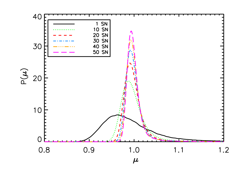
Figure 1.— Effective lensing magnification distributions for multiple perfect standard candles, at $z=1.5$ in a $\Lambda$CDM concordance cosmology. As more sources are observed the distribution approaches a Gaussian, and eventually converges on a $\delta$-function at the unlensed magnification, $\mu=1$.

The distributions at $z=1.5$, for various values of $N$, are shown in Figure 1. Note that even for as many as 50 SNe averaged together, the resulting distribution in magnification is still visibly asymmetric. This is a result of the high-magnification tail possessed by the lensing distributions. Figure 2 displays the shift of the mode of the distribution, as increasing numbers of SNe are observed. As expected, the curve asymptotes (slowly) to a value of 1, since the mean of the PDFs is always preserved, and for large numbers of SNe the PDF should be well sampled.

Figures 3 and 4 display the variance of the multiple SN lensing PDFs, as a function of the number of SNe. Since we are restricting our attention to smoothly clustered dark matter (as opposed to point masses like MACHOs; see Amanullah (2003) for a treatment of that case), the variance for $P_{1}(\mu)$ remains well-defined and finite. The difference between $\sigma$ and the full width at half maximum (FWHM) determination of the width is further evidence of the non-Gaussianity of the underlying lensing distribution: for a perfect Gaussian, $\sigma={\rm FWHM}/2.36$. For $N=1$, the standard deviation is 1.61 times the FWHM/2.36. By $N=50$, this factor has gone down to 1.35, indicating a more Gaussian-like distribution.

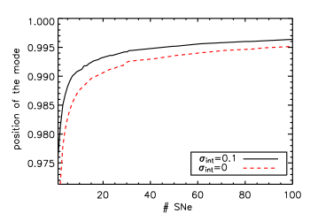
Figure 2.— Mode (peak) of the lensing magnification distributions for multiple standard candles (see Fig. 1), as a function of the number of SNe averaged together. For a Gaussian, the mode equals the mean. The (very slow) convergence to the mean (at 1) for many sources averaged together can be seen. This is shown both for perfect standard candles ($\sigma_{\rm int}=0$), and for SNe with intrinsic noise given by a Gaussian in flux with $\sigma_{\rm int}=0.1$. This is for SNe at $z=1.5$.

3.2. Sources with intrinsic luminosity dispersion

If the sources were perfectly calibrated candles, then the distribution of observed fluxes would exactly mirror those shown in Figure 1 (i.e., reflect only the lensing magnification suffered during propagation). However, astronomical sources, even calibrated candles such as Type Ia supernovae, retain some intrinsic variation in their luminosity. This gives an innate a priori fuzziness in the distance-redshift relation, and the observed relation is thus a convolution of both the intrinsic and lensing flux distributions. In other words, the distribution of observed flux, $F$, is given by

$$P(F) = \int dF_{0}\int d\mu\,p^{\rm int}(F_{0})\,p^{\rm lens}(\mu)\,\delta(F-F_{0}\mu)$$ (6)

$$= \int{d\mu\over\mu}\,\,p^{\rm int}\!\left(\frac{F}{\mu}\right)p^{\rm lens}(\mu),$$ (7)

where $F_{0}$ is the intrinsic source flux. In terms of magnitudes, the PDF for a single lensed, imperfect standard candle is given by

$$P^{\rm int+lens}(m)=\int d\mu\,P^{\rm lens}(\mu)\,P^{\rm int}(m+2.5\log\mu).$$ (8)

To form the N-fold convolution of N lensed, imperfect standard candle SNe, one takes the lensing + intrinsic, single SN PDF of equation (7) as $P_{1}$, and plugs this into equation (4) or (5). As before, the normalization and mean of $P_{1}$ are preserved for $P_{N}$.

For the intrinsic supernova flux distribution we consider both a Gaussian in magnitude (which corresponds to a log normal in flux) and a Gaussian in flux. The SN distribution is characterized by a mean intrinsic magnitude ($\left<m(z)\right>=m_{0}(z)$ or $\left<\mu(z)\right>=1$), and an intrinsic dispersion, $\sigma_{\rm int}(z)$. Canonically one uses $\sigma_{\rm int}(z)=0.1$ or $0.15$ (constant with redshift). Figures 2–4 show the resulting mode and variance, as a function of the number of observed SNe, for intrinsic noise given by a Gaussian in flux with standard deviation given by $\sigma_{\rm int}=0.1$. Note that the addition of intrinsic noise to the sources decreases the shift in the mode of the magnification PDF, but increases the variance.

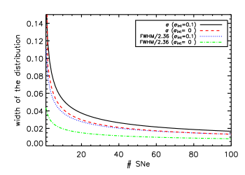
Figure 3.— Width of the lensing magnification distributions for multiple standard candles (see Fig. 1), as a function of the number of SNe averaged together. This is computed both as a variance, $\sigma^{2}$, and as a full-width half-maximum, FWHM. For a Gaussian, one has $\sigma=\mbox{FWHM}/2.36$. The gap between the $\sigma$ and FWHM curves is an indication of the non-Gaussianity of the lensing distributions. This is shown both for perfect standard candles ($\sigma_{\rm int}=0$), and for SNe with intrinsic noise given by a Gaussian in flux with $\sigma_{\rm int}=0.1$. This is for SNe at $z=1.5$.

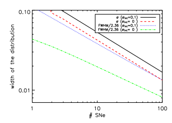
Figure 4.— As in Fig. 3, but on a log-log plot. The slopes of the standard deviation curves are very close to $-1/2$, indicating that the variance of the magnification distribution, including lensing, scales as $1/N$.

3.3. Lensing as a function of redshift

The previous section concerned itself with the distribution of the observed flux of multiple supernovae, averaged together. These distributions are of interest because they emphasize that lensing preserves the mean (unlensed) flux, and thus for sufficient numbers of observed SNe the lensing can be averaged away. Figure 1 is a visual representation of the process of convergence to successively narrower Gaussians, approaching the delta-function limit.

Guided by this convergence, we define an effective variance, $\sigma_{\rm eff}^{2}$, due to lensing. Consider some large number of standard candles, $N$, observed at a given redshift. For sufficiently high $N$, the lensing distribution is found to be well-approximated by a Gaussian. If we designate the variance of this Gaussian as $\sigma_{N}^{2}$, we can then define the effective variance due to lensing, for a single standard candle, as $\sigma_{\rm eff}^{2}=N\sigma_{N}^{2}$. Although the true distribution of a single standard candle is not well-described by a Gaussian of standard deviation $\sigma_{\rm eff}$, Figure 4 indicates that the scaling of the variance $\sigma_{N}^{2}$ is roughly inverse linear in $N$. So $\sigma_{\rm eff}$ gives an equivalent dispersion for each source when considering sufficiently large, but finite, numbers of standard candles. A useful rule of thumb for a reasonable use of $\sigma_{\rm eff}$ is to require $N$ greater than some lower limit calculated by demanding that $\sim$95% of the probability of the $N$-folded PDF be within $2\sigma_{N}$; this yields values of $N\gtrsim 10$.

As SNe do not all occur at exactly the same redshift, we need to know over what redshift width we can apply this criterion. As we take SNe spread out in redshift, the lensing PDFs, and hence $\sigma_{\rm eff}$, vary. If we bound this variation such that the 95% criterion above only dilutes to a $95\pm 1$% criterion, this is equivalent to using a $2\pm 0.1\,\sigma_{N}$ allowance. So we may group SNe within a 5% fractional deviation in $\sigma_{N}$; since as we will see below, the standard deviation is linearly proportional to redshift, this imposes $\Delta z/z\lesssim 0.05$. In other words, so long as there are $N\gtrsim 10$ SNe in each redshift bin of width $0.1z$, the lensing can be effectively described by a Gaussian with standard deviation $\sigma_{\rm eff}$. (We emphasize that none of this necessitates any actual binning for the SN analysis.) For SNe that are more sparse in redshift, the full non-Gaussian lensing PDF should be used. Sufficient numbers allow lensing to be treated as a scaled noise added in quadrature; greater numbers of SNe are required to compensate for this noise—see §4.

Lensing has little impact at low redshifts, where a short propagation distance implies a low optical depth. As the distance to the source increases, the lensing effects become more substantial. We thus expect $\sigma_{\rm eff}$ to increase with redshift. Figure 5 plots $\sigma_{\rm eff}$ as a function of $z$, for perfect standard candles, and for supernovae with intrinsic noise given by a Gaussian in flux with $\sigma_{\rm int}=0.1$. The results can be well approximated by a linear fit:

$$\sigma_{\rm eff}=0.088z,$$ (9)

for the case of perfect standard candles. In terms of magnitudes, we find

$$\sigma_{\rm eff,m}=0.093z$$ (10)

(to be used if taking $\sigma_{\rm int}$ as Gaussian in magnitude).

4. Cosmological Parameter Estimation in the Presence of Lensing

To map the expansion history of the Universe and reveal properties of the dark energy, next generation experiments are being designed to observe the luminosity distance-redshift curve to one percent precision out to high redshift; for example, this is a primary science goal of the Supernova/Acceleration Probe (SNAP; Aldering et al., 2004). From the cosmological inverse square law the luminosity distance, $d_{L}$, is related to the flux magnification, $\mu$, by $\mu\sim d_{L}^{-2}$. The errors on distance are then given by $\delta d_{L}/d_{L}=(-1/2)\delta\mu/\mu\sim\sigma_{\mu}/2$. It follows from §3 (e.g., see Fig. 5) that the distance dispersion due to gravitational lensing of any given SN at $z\gtrsim 0.5$ is of order or greater than one percent. Figures 1–4 illustrate the way to overcome this noise: observations of sufficient numbers of SNe per redshift “bin” convert a high-dispersion, non-Gaussian lensing distribution to a narrow, Gaussian-like one. For example, according to Figure 3, in order for lensing to contribute less than 1% distance uncertainty at $z=1.5$ requires $\sim 70$ SNe (with $\sigma_{\rm int}=0.1$), as compared to $25$ SNe if there were no lensing.

It is to be noted that, since gravitational lensing is achromatic, the redshifts of the sources are unaffected. Thus the effects of lensing are confined to changing the inferred luminosity distance. This compromises the determination of the luminosity distance-redshift curve, and thus impacts the estimation of cosmological parameters.

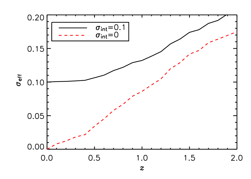
Figure 5.— The effective standard deviation in flux (see text) is plotted as a function of redshift, including lensing. For perfect standard candles (dashed (red) line) this illustrates the pure lensing contribution; also plotted is the convolution with SN intrinsic dispersion given by a Gaussian with standard deviation 0.1 in flux (solid (black) line).

4.1. Fisher approximation

Given an observable quantity, and a model for its measurement errors, the most straightforward method for generating constraints on dependent cosmological parameters is the Fisher matrix approach. For a supernova survey, the data consists of magnitudes at several redshifts, and the Fisher matrix is

$$F_{ij}=\sum_{z}\frac{\partial\langle m\rangle(z)}{\partial\theta_{i}}\frac{\partial\langle m\rangle(z)}{\partial\theta_{j}}\frac{N(z)}{\sigma_{m}^{2}(z)},$$ (11)

where $N(z)$ is the number of supernovae in a redshift bin. This formalism can treat both offset effects in the observed magnitudes $\langle m(z)\rangle$ and dispersion effects in $\sigma_{m}$.

We take as a set of cosmological parameters $\theta_{i}=\{{\mathcal{M}},\Omega_{m},w_{0},w_{a}\}$, where ${\mathcal{M}}$ is a nuisance parameter involving the absolute magnitude of the supernova and the absolute distance scale (i.e. the Hubble constant), $\Omega_{m}$ is the dimensionless matter density (we assume a flat Universe), and $w_{0}$ and $w_{a}$ parametrize the dark energy equation of state ratio $w(z)=w_{0}+w_{a}(1-a)$.

As a fiducial cosmology we adopt $\Omega_{m}=0.28$, $w_{0}=-1$, and $w_{a}=0$, and either include a Gaussian prior of $\sigma(\Omega_{m})=0.03$ or a WMAP cosmic microwave background constraint on the distance to the last scattering surface. We also explore variations of the fiducial model.

The increased magnification dispersion from lensing, as a function of redshift, is shown in Figure 5, and given in the fitting function of equation (10). The total dispersion $\sigma_{m}(z)$ is then obtained by adding in quadrature the intrinsic SN luminosity dispersion and the lensing effect:

$$\sigma_{m}^{2}(z)=\sigma_{{\rm eff},m}^{2}(z)+\sigma_{\rm int}^{2}.$$ (12)

One can verify from Figure 5 that the fitting form convolved with the intrinsic dispersion is a good approximation to the full, numerical solution.

Before we study the effect of the increased dispersion on determination of cosmological parameters, we obtain a first indication of the influence of lensing by asking how many supernovae are required to offset the increased dispersion. We can then correct for this extra scatter by increasing the sample size. If we want the magnitude scatter to be at the same level as if there were no lensing, then we observe extra supernovae such that

$$N(z)=N_{0}(z)\,\sigma_{m}^{2}(z)/\sigma_{\rm int}^{2}.$$ (13)

From equations (10) and (12) with $\sigma_{\rm int}=0.1$, 0.15, we find that the excess numbers required are $\Delta N/N_{0}=(z/z_{*})^{2}$ with $z_{*}=1.08$, 1.61 respectively (i.e., in the bin around $z_{*}$ half of the SNe are simply going to offset the increased lensing dispersion). Figure 6 illustrates this “survey bloat”, or conversely the degradation factor in the effectiveness of $N$ SNe. At $z=1.5$ one requires nearly three times as many SNe (with intrinsic dispersion $\sigma_{\rm int}=0.1$ in flux) to obtain the same dispersion as the case without lensing. In other words, each $z=1.5$ SN has $1/3$ the statistical weight it would have had in the absence of gravitational lensing.

For sufficient number of SNe (given by the degradation factor in eq. 13), however, lensing dispersion has no ill effect on cosmological parameter estimation. Furthermore, because the cosmological leverage occurs not merely from the highest redshift SNe, but from SNe at all intermediate redshifts as well, the relevant degradation factor is much more modest than suggested in Figure 6. For a fiducial distribution of 40 low redshift SNe, 10 per 0.1 bin at medium redshift, and 1 per 0.1 bin at high redshift (with no systematic uncertainties other than lensing), and adding a 0.03 prior on $\Omega_{m}$, the effect of lensing from equation (12) is a 15–20% weakening of the constraints on $w_{0}$ and $w_{a}$. Furthermore, this can be undone by increasing uniformly the number of SNe in each bin by a factor of 1.4, not the factor of three suggested by Figure 6 for $z=1.5$ alone. (These numbers hold with the further addition of a WMAP prior on distance to the last scattering surface. For a fiducial cosmology with SUGRA dynamical dark energy ($w_{0}=-0.82$ and $w_{a}=0.58$), rather than a cosmological constant, the weakening is 20–30%, though now a WMAP prior helps reduce it to 5–7%.)

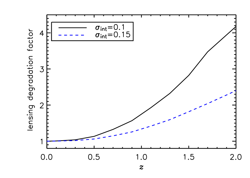
Figure 6.— Degradation factor due to gravitational lensing, as a function of redshift. This gives the fractional increase in the number of standard candles to be observed, to reduce the dispersion to what would have been observed without lensing. This is shown for two values of the SN intrinsic noise, given by Gaussians in flux.

In addition to dispersion, lensing leads to a skewness in the convolved flux distribution. For a large sample this is not worrisome since lensing preserves the mean flux; a proper SN cosmology analysis treats the data in flux (though it may be quoted in terms of magnitude), and so there is no offset in the mean (see Appendix A for a discussion of bias induced by flux-magnitude confusion). But if the distribution is not well sampled then one might find a magnification offset from the mean. We characterize this by the mode of the distribution, which will be shifted to magnification lower than unity. Such an offset would affect cosmological parameter determination, and we can calculate this within the Fisher matrix formalism. Figure 7 shows the mode offset, reasonably fit for a SN with $\sigma_{\rm int}=0.1\mbox{ mag}$ by

$$\Delta m(z)=0.025\,(z-0.7),\qquad z>0.7$$ (14)

and zero shift for $z<0.7$.

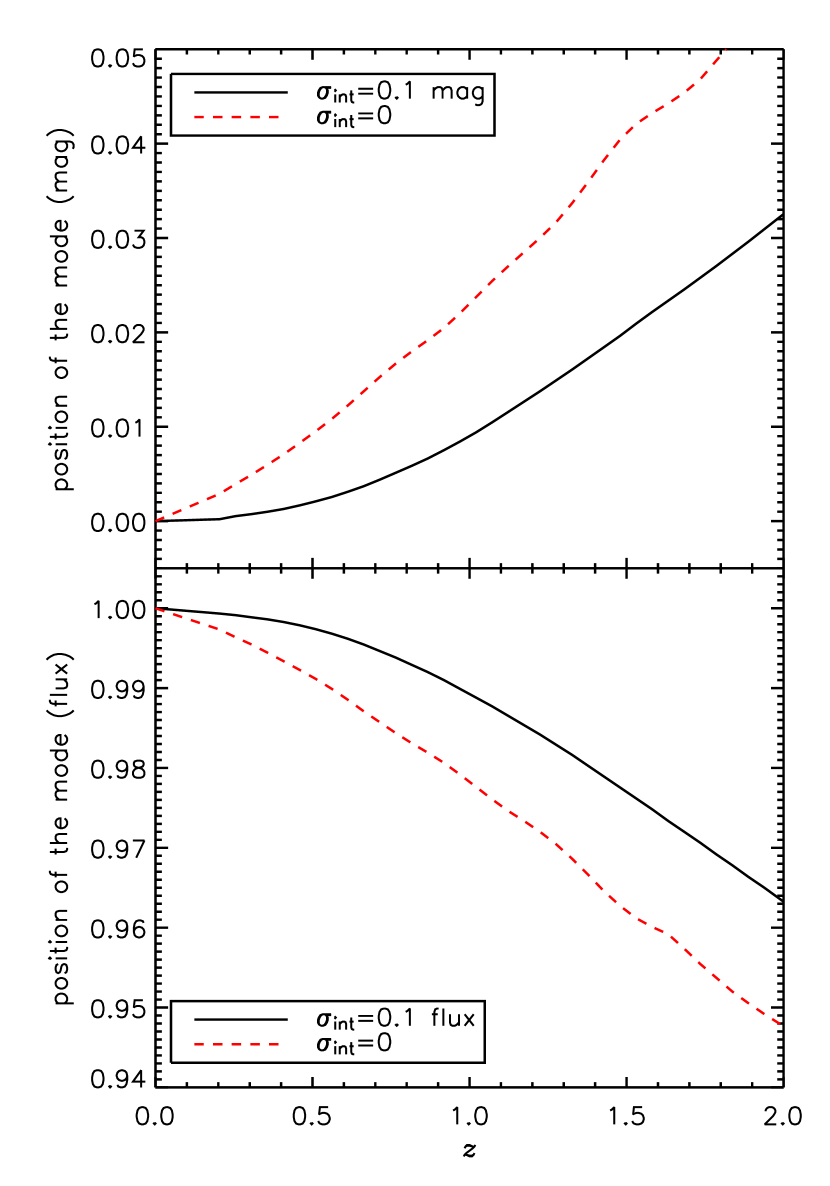
Figure 7.— The mode of the distributions, as a function of redshift. This is shown both in magnitude (upper panel) and flux (lower panel), for either SN intrinsic noise (in magnitude or flux, respectively), $\sigma_{\rm int}=0.1$ (solid black), or perfect standard candles (dashed red).

Such an offset propagates into a cosmological parameter bias via

$$\Delta\theta_{i}=(F^{-1})_{ij}\int dz\,N(z)\,\Delta m(z)\frac{\partial m}{\partial\theta_{j}}\frac{1}{\sigma_{m}^{2}(z)},$$ (15)

and gives a bias of less than $0.2\sigma$ (for the SUGRA case as well), where $\sigma$ is the statistical error. Indeed, the shift of the mode is of even less concern in that equation (14) refers to a single SN. For $N$ SNe at a given redshift, we expect the magnification distribution to approach a Gaussian, and hence the mode to approach unity, with its deviation diminishing as $1/\sqrt{N}$. This behavior is demonstrated in Figure 2. Since the Fisher matrix increases proportionally with $N$ (it is also known as the information matrix), then from equation (15) we see that the parameter bias will scale as the mode offset, and thus vanishes as $N^{-1/2}$. For the number of SNe in current data sets, the lensing bias makes little difference (unlike the flux-magnitude asymmetry; see Appendix A) due to the large statistical error, but as the number of SNe increases the scaling will make the mode offset effect essentially negligible.

The overall conclusion of the Fisher analysis is that lensing is a relatively benign error. It is of significance only at high redshifts ($z>1$), where there are currently few SNe measurements, and so large statistical errors, and hence only modest cosmological leverage. Once many high-$z$ SNe are observed, however, then lensing again is not a major source of error since the mean magnification averages to unity. Only when there are merely a handful of high redshift SNe per bin will lensing play a significant role.

4.2. Monte-Carlo simulations

While the Fisher analysis of the previous subsection gives a simple, intuitive feel for the effect of lensing on cosmological parameter determination, there remains the issue of the non-Gaussian nature of the gravitational lensing signal. A more robust, if computationally intensive, approach is to directly simulate data sets, and explore the ensuing scatter in best-fit parameter space. This presumes that the likelihood of a set of derived parameters, given an observed data set, is equivalent to the probability of observing a data set, for a given set of parameters.

We specify a cosmology, and calculate the lensing distribution via the SUM approach. We then simulate an “observed” data set, with the SNe at pre-defined redshifts, and the intrinsic and lensing noise for each SN drawn randomly from the appropriate distribution. For each data set we find the best-fit cosmology (using a maximum likelihood approach). We repeat this procedure for many ($\sim$40,000) simulated data sets, and draw contours in parameter space encompassing the distribution of best-fit models (e.g. the $1\sigma$ contour is the smallest contour which encompasses $68\%$ of the simulated data sets).

Figure 8 shows the resulting $1\sigma$ and $2\sigma$ contours, for a SN set roughly representing the current data (see the caption for details). The presence of lensing makes only a slight difference in the contours. This is because the data set under consideration has a small number of high-redshift ($z>1$) SNe, and so the effects of lensing are mitigated. At $3\sigma$, however, lensing has a more significant influence, greatly increasing the dispersion. In addition, lensing due to compact objects (MACHOs, e.g. solar-mass black holes), will have a greater impact. We consider the extreme case of $1/4$ of the dark matter in compact objects, representing the maximum reasonable lensing effects for a given cosmology. The outermost (dotted) set of contours illustrate this extreme case; the additional lensing leads to a $\sim 30\%$ degradation of the parameter estimation (also see Appendix B on clumpy lensing).

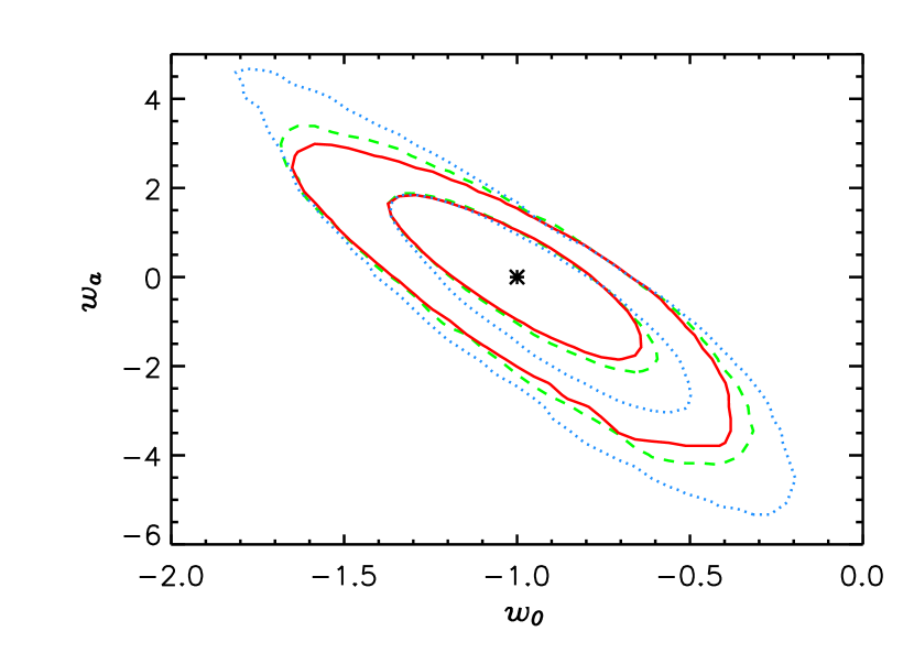
Figure 8.— Comparison of contours in parameter space, both with and without lensing. This is for observations of 20 SNe evenly distributed in the range $0.01<z<0.1$, 20 SNe in $0.1<z<0.5$, 8 SNe in $0.5<z<0.9$, and 8 SNe in $1<z<1.7$. The intrinsic dispersion of the supernovae is taken to be a Gaussian in magnitude with standard deviation given by $\sigma_{\rm int}=0.1\mbox{ mag}$, with a prior on $\Omega_{m}$ given by $\Omega_{m}=0.28\pm 0.03$. This data set is roughly comparable to the current state of SN observations (which are statistically more numerous, but with greater individual errors). Solid (red) contours are without lensing. Dashed (green) contours include lensing effects. Dotted (blue) contours represent an extreme lensing scenario, where 1/4 of the dark matter is in compact objects (MACHOs).

The moral to be drawn from this figure is that lensing is unlikely to have dramatic effects on the cosmological parameters estimated from current supernova data. A similar conclusion holds if one adopts a CMB prior rather than a matter density prior. However, we expect increasing influence of lensing as observations attain higher redshifts, but have not yet achieved sufficient numbers of supernovae to compensate for the lensing degradation.

Figure 9 shows that once high redshift surveys do observe many supernovae, the effective dispersion formula of equation (9) provides good insight, and the Fisher matrix formalism, properly handled, can give a reasonable approximation. With 100 SNe at $z=1$ and 100 at $z=1.5$, the contour including lensing is bloated by 30% in $w_{0}$ and 20% in $w_{a}$ relative to a Universe without lensing. The Monte Carlo contour can be predicted by using the appropriate $\sigma_{\rm eff}$, or equivalently degraded number of SNe.

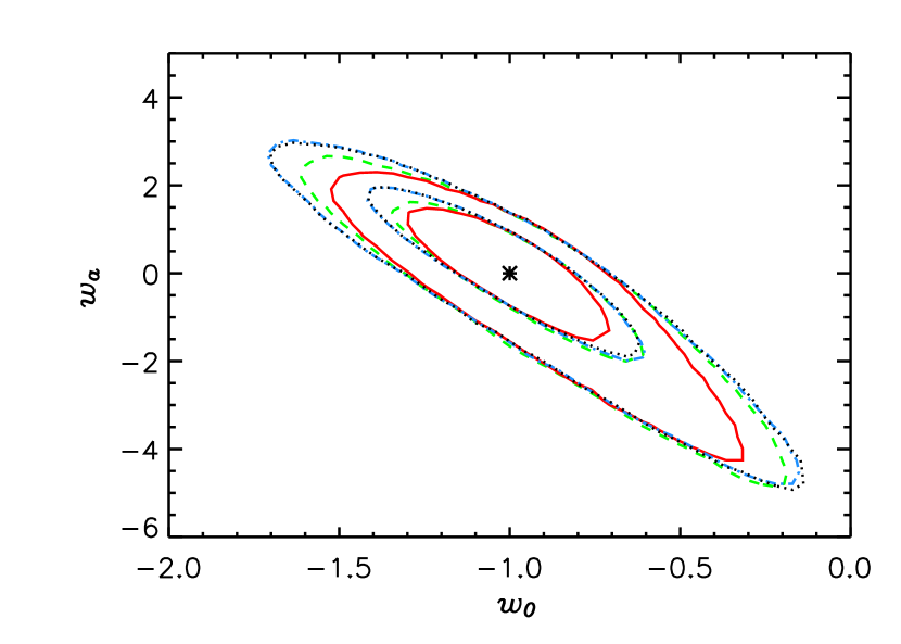
Figure 9.— At redshifts $z\geq 1$, lensing effects become more significant. With sufficient numbers of supernovae, however, the effects can be treated via a Gaussian effective dispersion, or number degradation factor, and well approximated with the Fisher matrix formalism. Here contours represent parameter estimation from 40 SNe at $z<0.1$, 100 SNe at $z=1$, and 100 at $z=1.5$, including a prior on $\Omega_{m}$ given by $\Omega_{m}=0.28\pm 0.03$. The solid (red) contours are for SNe with intrinsic dispersion given by a Gaussian in magnitude with standard deviation $\sigma_{\rm int}=0.1\mbox{ mag}$, without any gravitational lensing effects considered. The dashed (green) contours are for the same data set, but with the effects of lensing included through Monte Carlo of the PDF. The dotted (black) contour represents the $\sigma_{\rm eff}$ case (see §3.3), where the same SN data set is considered, with the lensing effects approximated by an increased Gaussian intrinsic dispersion in magnitude for the SNe (see eq. (12)). The dot-dashed (blue) contours demonstrate the degradation factor (see §4.1). This is for SNe with intrinsic noise given by $\sigma_{\rm int}=0.1\mbox{ mag}$, but with the lensing approximated by a diminution in the number of SNe, in accordance with eq. (13), yielding 54 SNe at $z=1$ and 34 SNe at $z=1.5$. As expected, the $\sigma_{\rm eff}$ and “degradation” contours are essentially indistinguishable.

Specifically, we see that the lower right half of the Monte Carlo lensing contour (dashed (green) curves) matches the Monte Carlo contours generated without the presence of lensing, but with dispersion corresponding to $\sigma_{\rm eff}$ added in quadrature (dotted (black) curves), or with merely intrinsic dispersion but numbers degraded by the appropriate factor from equation (13) (dot-dashed (blue) curves). The upper left half of the lensing contour is not as extended, and approaches a Monte Carlo contour generated without lensing (solid (red) curves).

We can understand this as follows: The models toward the lower right have equation of state ratios $w<-1$ at redshifts $z\gtrsim 1$ (where lensing is important). For such values of $w$, the SNe should be dimmer than for our fiducial model. However, lensing magnification, $\mu>1$, can offset this dimming and make these models of nearly equal likelihood to the fiducial—i.e. they will lie within the confidence level contour. For models toward the upper left, on the other hand, the opposite obtains: $w>-1$ and $\mu<1$. The $\mu>1$ part of the lensing PDF, convolved with the intrinsic PDF, is well represented in its cosmological effects by a Gaussian with $\sigma_{\rm eff}$. The $\mu<1$ part, even after convolution, is narrower due to the sharp low $\mu$ behavior of the lensing PDF, and so gives a Gaussian with dispersion closer to $\sigma_{\rm int}$. This can be understood physically: gravitational lensing imposes a lower limit to the amount of demagnification, given by the empty-beam value (e.g., there is a minimum amount of focusing due to matter along any line-of-sight, given by the vacuum value). There is no similar limit to the magnification side. Thus, lensing is by its nature asymmetrical, and this is reflected in the contours. Note, however, that both sides can independently be reasonably approximated by the Fisher formalism with the appropriate dispersions.

This general agreement is despite the fact that the PDF has not yet converged to a Gaussian form. Figure 10 clearly indicates that visible non-Gaussianity remains in the probability distribution even with 100 SNe at $z=1.5$: the lensing PDF is skewed from a Gaussian with the same variance (solid (black) curve vs. dashed (red) curve), and the variance is significantly different from the FWHM/2.36 (dotted (blue) curve is a Gaussian with the same FWHM as the lensing PDF). Thus, both the mode and the width of the magnification distribution exhibit non-Gaussianity—the central limit theorem still has a ways to go. Note, though, that the mean values for all the distributions agree (at the (unlensed) value of 1), and Figure 9 indicates that the cosmological parameter estimation is only dependent on broad characteristics of the lensing PDF, sufficiently described by our $\sigma_{\rm eff}$.

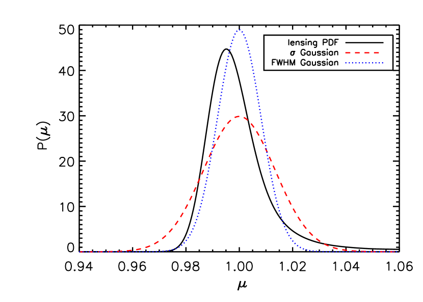
Figure 10.— When many high redshift sources are observed, the lensing magnification distribution will approach a Gaussian and eventually converge on a $\delta$-function at the unlensed magnification, $\mu=1$. However, this convergence can be slow; the solid (black) curve shows the PDF for 100 SNe at $z=1.5$. Residual non-Gaussianities are clear: the lensing PDF shows deviations from both the dashed (red) curve representing a Gaussian with the same variance, and the dotted (blue) Gaussian distribution with the same full width at half maximum. However, we find that these residuals do not substantially affect cosmological parameter estimation, and it can be sufficient to account for lensing by means of a Gaussian effective dispersion $\sigma_{\rm eff}$.

5. Conclusion

Cosmological observations of the distance-redshift relation of Type Ia supernovae have revealed an extraordinary new component in the Universe: dark energy. To explore this in detail, we must comprehend the astrophysics that factors into the measurements and their interpretation. Realistic assessment of the data from large surveys over the next decade requires consideration of a realistic Universe. Structure on various scales fills the Universe, and every light ray is affected at some level by the resulting gravitational lensing.

We have presented quantitative calculations of lensing effects on cosmological parameter estimation through observation of the luminosity distance-redshift relation. Using a Monte Carlo simulation code we derived the lensing magnification probability distribution function, and investigated its non-Gaussian characteristics, its behavior as the number of sources increased, and its redshift dependence. All of these have important ramifications for the interpretation of high-redshift observations.

In particular, above redshift $z\simeq 1$ lensing has a significant effect, degrading the statistical weight of sources by factors that exceed two (i.e. each source has less than $1/2$ the cosmological leverage of one in a Universe without lensing), and increasing roughly as $z^{2}$. Standard candles at redshifts $z\gtrsim 2$ will be severely impacted unless several hundreds can be observed at each redshift; this seems to doom hypothetical ultra-high-redshift standard candles such as gamma ray bursts or gravitational waves from inspiraling black holes (see Hughes & Holz (2003); Holz & Hughes (2004) for a similar conclusion).

We provide useful fitting formulas for the effective luminosity variance and mode offset induced by lensing, as a function of redshift, and compute their influences on cosmological parameter determination, checking these against Monte Carlo simulations. Lensing effects, though still appreciably non-Gaussian even with 100 sources at a given redshift $z>1$, can be well approximated by fitting functions for $N\gtrsim 10$ sources (within $\sim 0.1z$). The fitting function for the flux dispersion induced by lensing is given by:

$$\sigma_{\rm eff}=0.088z.$$ (16)

From this expression, and from direct numerical calculations, we find that $N\approx 70$ sources are needed to achieve 1% distance measurements at $z=1.5$. This effective dispersion formalism, combined with the flux conserving properties of lensing (the mean magnification is unity), tells us that while lensing certainly cannot be ignored, it is tractable, with safety in numbers.

Appendix A Non-Gaussianity: Log-normal approximation and flux vs. magnitude

While the full lensing PDFs derived from Monte Carlo simulations within the Stochastic Universe Method encapsulate the effects of structure on the luminosity distance-redshift relation, it is also useful to consider a simple approximation exhibiting non-Gaussianity. This will allow derivation of a number of analytic relations and help provide insight.

Since astronomical observations of supernovae use a logarithmic flux system of magnitudes, with $m=-2.5\log_{10}F$, it is natural to investigate a log normal distribution as a stand-in for the lensing magnification. This in fact has several attractive properties: a natural skewness, simple characterization, and Gaussian behavior near the peak. We do not claim it fits the derived lensing PDF, only that it has some related properties.

A log normal probability distribution has the form

$$p(\mu)=\frac{1}{\sqrt{2\pi}}\frac{1}{S\mu}e^{-(\ln\mu-U)^{2}/(2S^{2})},$$ (A1)

and possesses mean $\langle\mu\rangle=e^{U+S^{2}/2}$, with mean logarithm $\langle\ln\mu\rangle=U$, and variance $\sigma_{\mu}^{2}=\langle\mu^{2}\rangle-\langle\mu\rangle^{2}=e^{S^{2}}-1$. Note that from the physical interpretation of the magnification, flux conservation ensures that $\langle\mu\rangle=1$, and so for our case $U=-S^{2}/2$. Thus we have a one parameter PDF with $\langle\ln\mu\rangle<0$, skewed negative as desired.

We can now evaluate equation (7) and find that the convolution distribution for the observed flux is also a log normal distribution, broader and with different skewness:

$$P(F)=\frac{1}{\sqrt{2\pi}}\frac{1}{\sqrt{S^{2}+\sigma_{\rm int}^{2}/b^{2}}}\frac{1}{F}e^{-(\ln F+m_{0}/b-U)^{2}/[2(S^{2}+\sigma_{\rm int}^{2}/b^{2})]},$$ (A2)

where $b=2.5/\ln 10$ converts from flux in natural log to magnitudes. The mean flux is $F_{0}$, and the mean of the logarithmic flux is

$$\langle\ln F\rangle=-\frac{\ln 10}{2.5}m_{0}+U=\langle\ln F_{0}\rangle+\langle\ln\mu\rangle.$$ (A3)

For observations using magnitudes, it is convenient to convert to the distribution in magnitude, $m$:

$$P(m)=\frac{1}{\sqrt{2\pi}\,\sigma_{m}}e^{-(m-m_{0}+bU)^{2}/(2\sigma_{m}^{2})},$$ (A4)

where $\sigma_{m}^{2}(z)=\sigma_{\rm int}^{2}+b^{2}S^{2}$. Also, recall that from flux conservation $U=-S^{2}/2$. Thus these probability distributions for source properties and lensing effects lead to a particularly simple result for the observed magnitude-redshift relation: there is an increased dispersion $\sigma_{m}$, and an offset in the mean. Explicitly,

$$\langle m\rangle(z) = m_{0}(z)-bU(z)$$ (A5)

$$\sigma_{m}^{2}(z) = \sigma_{\rm int}^{2}-2b^{2}U(z).$$ (A6)

Recall that $U<0$. The increased dispersion will weaken cosmological parameter determination, and the offset in the mean will bias the derived parameters. The magnitude of the effect is controlled by the quantity $U=\langle\ln\mu\rangle$. For example, the variance is doubled, relative to a 0.1 mag intrinsic dispersion, for $U=0.004$.

It is worth noting that no actual lensing is required to generate bias in the cosmological parameter determination. Image intensity can be expressed in either flux or magnitude, and the transformation between these systems of measurement gives a similar form of non-Gaussianity—that of the log normal distribution—with the attendant dispersion and bias. By confusing flux and magnitude values in an analysis of SN data, it is possible to severely compromise the values of the resulting cosmological parameters. Observing sources given by the numbers and redshifts in Riess et al. (2004), with an intrinsically Gaussian flux distribution, but interpreting them in terms of magnitudes, turns a true flat cosmology with $\Omega_{m}=0.28$ and a cosmological constant into an apparently substantially closed cosmology ($\Omega_{k}\approx 0.2$). This might also be interpreted as a flat model with a dark energy different from $w_{0}=-1$, $w_{a}=0$, in particular $w_{0}<-1$, $w_{a}>0$. To avoid bias one must therefore carry out both the observations and the analysis in a fully consistent manner (Holz, Livio, & Riess, 2004).

Appendix B Clumpy Universe model

The central problem of incorporating lensing effects from structure in the Universe into the distance-redshift relation is calculation of the magnification probability distribution function (see §2 of the main text). The simplest distribution of lensing magnifications, however, is no distribution at all. This is the approach of the clumpy Universe model of Dyer & Roeder (1973). This model does not ignore lensing, but rather assumes a special set of lines of sight—those that avoid mass concentrations. This preferentially avoids magnifications greater than unity. To conserve mass the model partially evacuates most of space, leaving an average density $\alpha\rho$, where $\alpha$ is the smoothness parameter and $\rho$ the globally averaged energy density, and concentrates the remaining mass into compact clumps that the “chosen” light rays never encounter. Furthermore, shear effects from these inhomogeneities are ignored. Thus the only light paths the observer deals with lead to demagnification ($\mu<1$) of the source, and overall flux is not conserved (we mention a way around this below).

We characterize this as shunning lensing rather than ignoring it, willfully neglecting data from sources touched by magnification; in general this is an even worse idea than completely ignoring lensing, due to the bias and flux nonconservation. However, we can use it as a simple, extreme case to examine the effect of lensing on the distance-redshift relation, and the ensuing cosmological parameter determination and bias (for example, see §4.2 and Fig. 8). Thus it is worth investigating some aspects of it here.

The distance-redshift relation is no longer an integral over the Hubble parameter, but instead becomes a second order differential equation following from the optical scalar equations. This was given for general equations of state by Kayser (unpublished, 1985) and Linder (1988), and can treat inhomogeneities not only in the matter but hypothetical clumpiness in the dark energy component. The effect of clumpiness enters the Ricci focusing as $[1+w(z)][1-\alpha_{w}(z)]\Omega_{w}(z)$, with $\alpha_{w}$ giving the ratio of smoothly distributed to total energy density in a component characterized by equation of state $w$.

We note several points: (1) a pure cosmological constant has no such Ricci focusing, (2) the effect is diminished as $w\to-1$ but is enhanced for larger $\Omega_{w}$, and (3) an evolving clumpiness can be treated straightforwardly (as detailed in Linder (1988)). One could certainly assume the canonical smoothness $\alpha_{w}=1$ for a component other than matter. However we can also explore more arcane models, such as postulating that dark energy couples to (dark) matter, or is affected through backreaction on the expansion from nonlinear structure formation in the matter. Thus we examine both $\alpha_{w}=1$ and $\alpha_{w}=\alpha_{m}$, where $\alpha_{m}$ is the clumpiness of the matter component. Since the clumpy Universe model generally counts larger scale structure such as galaxies and clusters as a smooth component, only excluding compact objects with strong magnifications, we take the conservative position that all dark matter is smooth, and about half of the baryons as well, so $\alpha_{m}=0.9$. The effects will be greater for more extreme cases. If we take as a dark energy model the SUGRA model with $w_{0}=-0.82$ and $w_{a}=0.58$, then at $z=0$ the Ricci focusing due to clumpy dark energy would be roughly half that due to clumpy matter. Continuing to be conservative, we henceforth ignore that contribution and assume the dark energy is smooth.

Before investigating the influence of clumpy lensing on cosmological parameter determination, let us consider parameter degeneracies. Recently, Caldwell & Kamionkowski (2004) pointed out that formally one could measure the curvature of space through the distance-redshift relation, with the curvature entering at third order in a low redshift expansion; however, the space geometry is entangled with the spacetime geometry, i.e. the expansion history. This usefully highlights the same point made in Linder (1988). Here we extend that result to show a six-fold degeneracy at ${\mathcal{O}}(z^{3})$ of the angular diameter distance:

$$r(z)\approx z-(1/2)(3+q_{0})z^{2}+z^{3}[2+(\Omega_{T}/4)(2+5\bar{w}-3\overline{w^{2}}-\overline{w^{\prime}}-\bar{\alpha}-\overline{w\alpha})+(1/2)q_{0}^{2}]+{\mathcal{O}}(z^{4}).$$ (B1)

The notation $\bar{X}=\sum_{w}X\Omega_{w}(0)/\Omega_{T}$, where $\Omega_{T}$ is the total dimensionless energy density, related to the curvature density by $\Omega_{k}=1-\Omega_{T}$ and to the deceleration parameter by $q_{0}=\Omega_{T}(1+3\bar{w})/2$. Thus one must know the average of the equation of state ratio $w$, of the time variation $w^{\prime}=dw/dz$, smoothness $\alpha$, etc. to determine the spatial curvature. This points up the well known necessity for distance observations at many redshifts over a long baseline, e.g. $z\approx 0-2$, to break the degeneracies and determine the cosmological parameters.

Let us consider such observations from a deep survey, corresponding to supernova observations from SNAP. If we shun lensing, but do not know the clumpiness of the Universe, then we introduce an additional fit parameter in the smoothness $\alpha$. While this increases the uncertainties in the other parameters, the more insidious effect is bias, or misestimation of the parameters. Within the context of a SUGRA model, assuming a smooth Universe while only utilizing lines of sight with $\alpha_{m}=0.9$ results in a bias to $w_{0}$ of $0.3\sigma$, and to $w_{a}$ of $0.8\sigma$, where $\sigma$ is the statistical precision. This gives a measure of the peril of shunning lensing, and an estimate of the damage of low statistics.

We emphasize that homogeneous observations that do not select special lines of sight do not run into such bias—it is better to ignore lensing than shun it, and best of all is to acknowledge and include it as done in this article. Could we form a probability distribution such as simulated in the Stochastic Universe Model from an analytic convolution of clumpy lines of sight? That is, could we incorporate both underdense and overdense lines of sight in such a way as to conserve flux and allow a simpler treatment than Monte Carlo analysis?

Two difficulties exist with this method. First, overdense lines of sight reach a limit at some critical $\alpha$, e.g. $\alpha>25/24$ for the flat, pure matter model, where the increased focusing forms caustics—i.e. the light rays focus before reaching the observer, and the angular distance vanishes there. But this can be overcome by analytic continuation. The second problem is that averaging must be done not in terms of density, i.e. restoring $\langle\alpha\rangle=1$, but in terms of flux conservation $\langle r_{\alpha}^{-2}\rangle=r_{FRW}^{-2}$, where FRW means a completely smooth, $\alpha=1$ Universe. This requires the use of a redshift dependent smoothness parameter, which can be managed, but it also becomes a recursive relation (cf. Linder (1988), Appendix C), which is no easier to deal with than the physically motivated PDF formalism used in the text of this paper.

Thus, our conclusions are that the Stochastic Universe Model, and the fitting functions we derive, offer the best way to realistically include lensing from the presence of structure in the Universe.

References

- Aldering et al. (2004) Aldering, G. et al. 2004, PASP, submitted [astro-ph/0405232]
- Amanullah (2003) Amanullah, R., Mörtsell, E., & Goobar, A. 2003, A&A, 397, 819 [astro-ph/0204280]
- Caldwell & Kamionkowski (2004) Caldwell, R.R. & Kamionkowski, M. 2004, JCAP, 0409, 9 [astro-ph/0403003]
- Dyer & Roeder (1973) Dyer, C.C. & Roeder, R.C. 1973, ApJ, 180, L31
- Frieman, Holz, & Knox (2005) Frieman, J.A., Holz, D.E., & Knox, L., in preparation
- Goobar et al. (2002) Goobar, A., Mörtsell, E., Amanullah, R., & Nugent, P. 2002, A&A, 393, 25 [astro-ph/0207139]
- Holz (1998) Holz, D.E. 1998, ApJ, 506, L1 [astro-ph/9806124]
- Holz (2001) Holz, D.E. 2001, ApJ, 556, L71 [astro-ph/0104440]
- Holz & Hughes (2004) Holz, D.E. & Hughes, S.A. 2004, [astro-ph/0212218]
- Holz, Livio, & Riess (2004) Holz, D.E., Livio, M., & Riess, A.G. 2004, in preparation
- Holz & Wald (1998) Holz, D.E., & Wald, R. M. 1998, Phys. Rev. D, 58, 063501
- Hughes & Holz (2003) Hughes, S.A. & Holz, D.E. 2003, Class. & Quant. Grav., 20S, 65
- Huterer & Ma (2004) Huterer, D. & Ma, C-P. 2004, ApJ, 600, L7 [astro-ph/0307301]
- Kayser (unpublished, 1985) Kayser, R. 1985, unpublished Ph.D. thesis
- Knop et al. (2003) Knop, R. A. et al. 2003, ApJ, 598, 102
- Kochanek (2004) Kochanek, C.S., Schneider, P. & Wambsganss, J. 2004, Part 2 of Gravitational Lensing: Strong, Weak & Micro, Proc. of 33rd Saas-Fee Advanced Course, eds. G. Meylan, P. Jetzer, P. North [astro-ph/0407232]
- Kuhlen, Keeton, & Madau (2004) Kuhlen, M., Keeton, C.R. & Madau, P. 2004, ApJ, 601, 104 [astro-ph/0310013]
- Linder (1988) Linder, E.V. 1988, A&A, 206, 190
- Linder (2003) Linder, E.V. 2003, Phys. Rev. Lett., 90, 1301
- Linder (2004) Linder, E.V. 2004, Phys. Rev. D, 70, 043534 [astro-ph/0401433]
- Metcalf & Silk (1999) Metcalf, R.B. & Silk, J. 1999, ApJ, 519, L1 [astro-ph/9901358]
- Oguri, Suto & Turner (2003) Oguri, M., Suto, Y. & Turner, E.L. 2003, ApJ, 583, 584 [astro-ph/0210107]
- Perlmutter et al. (1999) Perlmutter, S., et al. 1999, ApJ, 517, 565
- Phillips (1993) Phillips, M. M. 1993, ApJ, 413, L105
- Riess, Press, & Kirshner (1995) Riess, A. G., Press, W. H., & Kirshner, R. P. 1995, ApJ, 438, L17
- Riess et al. (1998) Riess, A., et al. 1998, AJ, 116, 1009
- Riess et al. (2004) Riess, A.G. et al. 2004, ApJ, 607, 665 [astro-ph/0402512]
- Seljak & Holz (1999) Seljak, U. & Holz, D.E. 1999, A&A, 351, L10 [astro-ph/9910482]
- Spergel et al. (2003) Spergel, D.N. et al. 2003, ApJS, 148, 175
- Tonry et al. (2003) Tonry, J. L. et al. 2003, ApJ, 594, 1
- Wang et al. (2003) Wang, L., Goldhaber, G., Aldering, G., & Perlmutter, S. 2003, ApJ, 590, 944
- Wang, Holz, & Munshi (2002) Wang, Y., Holz, D.E., & Munshi, D. 2002, ApJ, 572, L15