The stellar mass function of galaxies to $z\sim 5$ in the Fors Deep and GOODS-S fields

Abstract

We present a measurement of the evolution of the stellar mass function (MF) of galaxies and the evolution of the total stellar mass density at $0<z<5$, extending previous measurements to higher redshift and fainter magnitudes (and lower masses). We use deep multicolor data in the Fors Deep Field (FDF; $I$-selected reaching $I_{AB}\sim 26.8$) and the GOODS-S/CDFS region ($K$-selected reaching $K_{AB}\sim 25.4$) to estimate stellar masses based on fits to composite stellar population models for 5557 and 3367 sources, respectively. The MF of objects from the $K$-selected GOODS-S sample is very similar to that of the $I$-selected FDF down to the completeness limit of the GOODS-S sample. Near-IR selected surveys hence detect the more massive objects of the same principal population as do $I$-selected surveys. We find that the most massive galaxies harbor the oldest stellar populations at all redshifts. At low $z$, our MF follows the local MF very well, extending the local MF down by a decade to $10^{8}$ $\mathrm{M_{\odot}}$. Furthermore, the faint end slope is consistent with the local value of $\alpha\sim 1.1$ at least up to $z\sim 1.5$. Our MF also agrees very well with the MUNICS and K20 results at $z\lesssim 2$. The MF seems to evolve in a regular way at least up to $z\sim 2$ with the normalization decreasing by 50% to $z=1$ and by 70% to $z=2$. Objects with $M>10^{10}$ $\mathrm{M_{\odot}}$which are the likely progenitors of todays $L>L^{*}$ galaxies are found in much smaller numbers above $z\sim 2$. However, we note that massive galaxies with $M>10^{11}$ $\mathrm{M_{\odot}}$are present even to the largest redshift we probe. Beyond $z\sim 2$ the evolution of the mass function becomes more rapid. We find that the total stellar mass density at $z=1$ is 50% of the local value. At $z=2$, 25% of the local mass density is assembled, and at $z=3$ and $z=5$ we find that at least 15% and 5% of the mass in stars is in place, respectively. The number density of galaxies with $M>10^{11}\,\mathrm{M_{\odot}}$ evolves very similarly to the evolution at lower masses. It decreases by 0.4 dex to $z\sim 1$, by 0.6 dex to $z\sim 2$, and by 1 dex to $z\sim 4$.

1. Introduction

The stellar mass of galaxies at the present epoch and the build-up of stellar mass over cosmic time has become the focus of intense research in the past few years.

Generally, this kind of work relies on fits of multi-color photometry to a grid of composite stellar population (CSP) models to determine a stellar mass-to-light ratio, since large and complete spectroscopic samples of galaxies (at $z>0$) are not yet available.

In the local universe, results on the stellar mass function (MF) of galaxies were published using the new generation of wide-angle surveys in the optical (Sloan Digital Sky Survey; SDSS, York et al., 2000; 2dF, Colless et al., 2001) and near-infrared (Two Micron All Sky Survey; 2MASS, Skrutskie et al., 1997). Cole et al. (2001) combined data from 2MASS and 2dF to derive the local stellar MF, Bell et al. (2003) used the SDSS and 2MASS to the same end.

At $z>0$, a number of authors studied the stellar mass density as a function of redshift (Brinchmann & Ellis, 2000; Drory et al., 2001; Cohen, 2002; Dickinson et al., 2003; Fontana et al., 2003; Rudnick et al., 2003) reaching $z\sim 3$. It appears that by $z\sim 3$, about 30% of the local stellar mass density has been assembled in galaxies, and at $z\sim 1$, roughly half of the local stellar mass density is in place. This seems to be in broad agreement with measurements of the star formation rate density over the same redshift range.

Others investigated the evolution of the MF of galaxies (Drory et al., 2004; Fontana et al., 2004) to $z\sim 1.5$, finding a similar decline in the normalization of the MF. However, it is possible that galaxies evolve differently in number density depending on their morphology.

In this letter, we extend the measurement of the stellar MF and its integral, the total stellar mass density, to $z\sim 5$. We describe the data set in Sect. 2 and present the method used to derive stellar masses in Sect. 3. We discuss the results on the stellar MF in Sect. 4. Finally, we discuss the total stellar mass density and the number density of massive galaxies in Sect. 5.

Throughout this work we assume $\Omega_{M}=0.3$, $\Omega_{\Lambda}=0.7,H_{0}=70\ \mathrm{km\ s^{-1}\ Mpc^{-1}}$. Magnitudes are given in the AB system.

2. The galaxy sample

This work is based on data from two deep field surveys having multicolor photometry and rich followup spectroscopy, the Fors Deep Field (FDF; Heidt et al., 2003; Noll et al., 2004) covering the UBgRIzJKs bands in 40 arcmin² and the GOODS-S/CDFS field (Giavalisco et al., 2004) covering the UBVRIJHKs bands in 50 arcmin². This sample is identical to the one used in Gabasch et al. (2004b) to study the global star formation rate to $z\sim 5$.

The FDF photometric catalog is published in Heidt et al. (2003) and we use the I-band selected subsample covering the deepest central region of the field as described in Gabasch et al. (2004a). This catalog lists 5557 galaxies down to $I\sim 26.8$. The latter also discusses the I-band selection and shows that this catalog misses at most 10% of the objects found in ultra-deep K-band observations found by Labbé et al. (2003).

Photometric redshifts for the FDF are calibrated against 362 spectroscopic redshifts up to $z\sim 5$ and have a accuracy of $\Delta z/(z_{spec}+1)\leq 0.03$ with only $\sim 1$% outliers. The method and this calibration are presented and discussed in Gabasch et al. (2004a).

Our K-band selected catalog for the GOODS-S/CDFS field is based on the publicly available 8 $2.5\times 2.5$ arcmin² J, H, Ks ISAAC images, taken at ESO/VLT with seeing in the range $0.4^{\prime\prime}-0.5^{\prime\prime}$. The U and I images are from ESO GOODS/EIS public survey, while the B V R images are taken from the Garching-Bonn Deep Survey. These datasets are extensively discussed in Arnouts et al. (2001) and Schirmer et al. (2003), respectively.

The data for the GOODS field were analyzed in a very similar way to the data of the FDF. The objects were detected in the K-band images closely following the procedure used for the FDF I-band detection. A detailed description of the procedure as well as the catalogs can be found in Salvato et al. (2004, in preparation). We detect 3367 sources in the K-band for which we measure fixed aperture and Kron-like total magnitudes in all bands. Of these, 2 objects are detected only in K, and 36 objects are detected only in the Ks, H, and J band images. Number counts match the literature values down to $K\approx 25.4$, which is the completeness limit of the catalog. We computed photometric redshifts using the same method and SED template spectra as for the FDF. A comparison with the spectroscopic redshifts of the VIMOS team and the FORS2 spectra shows that the photometric redshifts have an accuracy $\Delta z/(z_{spec}+1)\leq 0.056$.

3. Deriving stellar masses

We derive stellar masses (the mass locked up in stars) by comparing multi-color photometry to a grid of stellar population synthesis models covering a wide range in parameters, especially star formation histories (SFHs). This method is described in detail and compared against spectroscopic and dynamical mass estimates in Drory, Bender, & Hopp (2004), hence we only briefly outline the method here.

We base our model grid on the Bruzual & Charlot (2003) models. We parameterize the possible SFHs by a two-component model, a main component with a smooth analytical SFH modulated by a burst of star formation. The main component is parameterized by a SFH of the form $\psi(t)\propto\exp(-t/\tau)$, with $\tau\in[0.1,\infty]$ Gyr and a metallicity of $-0.6<\mathrm{[Fe/H]}<0.3$. The age, $t$, (defined as the time since star formation began) is allowed to vary between 0.5 Gyr and the age of the universe at the object’s redshift. This component is linearly combined with a burst modeled as a 100 Myr old constant star formation rate episode of solar metallicity. We restrict the burst fraction, $\beta$, to the range $0<\beta<0.15$ in mass (higher values of $\beta$ are degenerate and unnecessary since this case is covered by models with a young main component). We adopt a Salpeter IMF truncated at 0.1 and 100 $\mathrm{M_{\odot}}$ for both components. A different slope will change only the mass scale. However, if the IMF depends on the mode of star formation the shape of the MF can be affected.

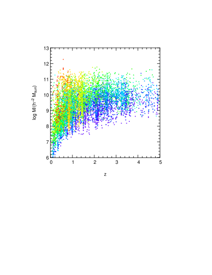
Figure 1.— Stellar masses vs. redshift in the FDF (squares) and in GOODS-S (triangles). The luminosity-weighted mean ages of the stellar populations as determined by the CSP fit are coded by colors ranging from red for old populations (age $\gtrsim 5$ Gyr) to blue for young populations (age $\lesssim 1.5$ Gyr).

Additionally, both components are allowed to exhibit a different and variable amount of extinction by dust. This takes into account the fact that young stars are found in dusty environments and that the starlight from the galaxy as a whole may be reddened by a (geometry dependent) different amount. In fact, Stasińska et al. (2004) find that the Balmer decrement in the SDSS sample is independent of inclination, which, on the other hand, is driving global extinction (Tully et al., 1998, see, e.g.,).

We compute the full likelihood distribution on a grid in this 6-dimensional parameter space ($\tau,\mathrm{[Fe/H]},t,A_{V}^{1},\beta,A_{V}^{2}$), the likelihood of each model being $\propto\exp(-\chi^{2}/2)$. To compute the likelihood distribution of $M/L$, we weight the $M/L$ of each model by its likelihood and marginalize over all parameters. The uncertainty in $M/L$ is obtained from the width of this distribution, which is on average between $\pm 0.1$ and $\pm 0.3$ dex at 68% confidence level. The uncertainty in mass has a weak dependence on mass (increasing with lower $S/N$ photometry) and much of the variation is in spectral type: early-type galaxies have more tightly constrained masses than late types. At high redshift, however, the uncertainty in $M/L$ grows as objects drop-out in the blue bands and stellar populations become younger: the typical uncertainty at $z\sim 3$ is 0.6 dex and becomes as large as 1 dex at the highest redshifts we probe.

In Fig.1 we show the distribution of galaxies in the mass vs. redshift plane for the FDF (squares) and GOODS-S (triangles). In addition, we code the age of each galaxy (using the best-fitting model) in colors ranging from blue for young (age $\lesssim 1.5$ Gyr) to red for old stellar populations (age $\gtrsim 5$ Gyr).

The distribution of objects from the $K$-selected GOODS-S sample is very similar to the distribution of the $I$-selected FDF down to the completeness limit of the GOODS-S sample, which is $\sim 1$ dex shallower in limiting mass. This indicates that present optical and near-IR surveys are unlikely to have missed a substantial population of massive objects, with the possible exception of heavily dust-enshrouded sources which may escape detection in both optical and near-IR surveys.

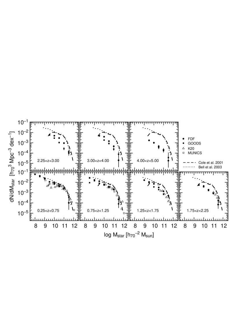
Figure 2.— The stellar mass function (MF) as a function of redshift. The local MF of Bell et al. (2003) and Cole et al. (2001) are shown in all redshift bins for comparison. Results from the MUNICS survey (Drory et al., 2004) and the K20 survey (Fontana et al., 2004) at $z\lesssim 2$ are also shown.

A striking feature of Fig.1 is that the most massive galaxies harbor the oldest stellar populations at all redshifts. There always exist galaxies which are old (relative to the age of the universe at each redshift) but less massive, yet the most massive objects at each redshift are never among the youngest.

4. The stellar mass function

Fig. 2 shows the $V_{\mathrm{max}}$-weighted mass function in seven redshift bins from $z=0.25$ to $z=5$. For comparison, we also show the local mass function (Bell et al., 2003; Cole et al., 2001) and the MFs to $z\sim 1.2$ of MUNICS (Drory et al., 2004) and to $z\sim 2$ by the K20 survey (Fontana et al., 2004).

The MF of objects from the $K$-selected GOODS-S sample is very similar to that of the $I$-selected FDF down to the completeness limit of the GOODS-S sample (with the exception of a possible slightly lower normalization at $z\gtrsim 2.5$ by about 10% to 20%). This shows that near-IR selected surveys at high redshift essentially detect the more massive objects of the same principal population as do optically ($I$-band) selected surveys (see also Sect. 3 and Fig. 1 in Gabasch et al., 2004a). It remains to be seen what fraction of massive galaxies (and total stellar mass density) might be hidden in dusty starbursts which appear as sub-mm galaxies.

In our lowest redshift bin, $z\sim 0.5$, the MF follows the local MF very well. The depth of the FDF ($I\sim 26.8$) allows us to extend the faint end of the MF down to $10^{8}$ $\mathrm{M_{\odot}}$, a decade lower in mass than in Bell et al. (2003), with no change of slope. Furthermore, the faint end slope is consistent with the local value of $\alpha\sim 1.1$ at least to $z\sim 1.5$. Our mass function also agrees very well with the MUNICS and K20 results at $z\lesssim 2$.

The MF seems to evolve in a regular way at least up to $z\sim 2$ with the normalization decreasing by 50% to $z=1$ and by 70% to $z=2$, with the largest change occurring at masses of $M~{}10^{10}$ $\mathrm{M_{\odot}}$. These likely progenitors of todays $L>L^{*}$ galaxies are found in much smaller numbers above $z\sim 2$. However, we note that massive galaxies with $M>10^{11}$ $\mathrm{M_{\odot}}$are present even to the largest redshift we probe (albeit in smaller numbers). Beyond $z\sim 2$ the evolution becomes more rapid.

It is hard to say whether the difference between the FDF and the GOODS-S field visible at $z\sim 3$ in Fig. 2 is significant. In fact, Gabasch et al. (2004b) find not much difference in the rest-frame UV luminosity function in the very same dataset. We think it might be related to the shallower near-IR data in the FDF compared to GOODS-S. Less reliable information on the rest-frame optical colors at young mean ages might in fact lead to an overestimation of the stellar mass. This would also explain why the two MFs become similar again at even higher $z$ when the near-IR data in GOODS-S reach their limit, too. This would mean that the mass density in the FDF at $z\gtrsim 2.5$ might be overestimated (see below).

5. Stellar mass density and number densities

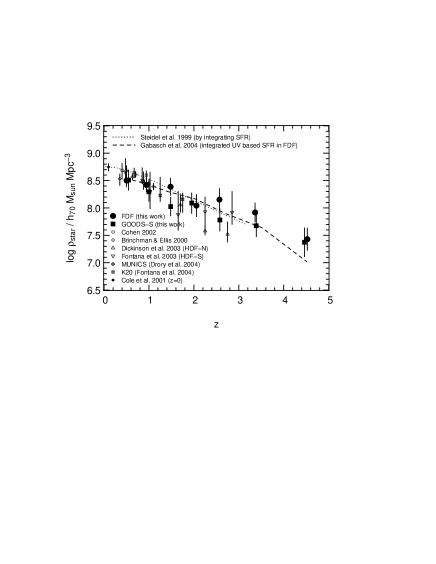
Figure 3.— The total stellar mass density of the universe as a function of redshift. We also show the integral of the star formation rate as a dotted line and dashed line.

Fig. 3 shows the evolution of the total stellar mass density along with data from the literature, extending the available data to $z\sim 5$ (Cole et al., 2001; Brinchmann & Ellis, 2000; Drory et al., 2001; Cohen, 2002; Dickinson et al., 2003; Fontana et al., 2003, 2004; Drory et al., 2004).

We compute the total stellar mass density by directly summing up contributions from all objects in both fields (we obtain very similar values by means of fitting Schechter functions to the data in Fig. 2). We find that the stellar mass density at $z=1$ is 50% of the local value as determined by Cole et al. (2001). At $z=2$, 25% of the local mass density is assembled, and at $z=3$ and $z=5$ we find that at least 15% and 5% of the mass in stars is in place, respectively. Fig. 3 shows the results from both fields separately, however.

We also show the integral of the star formation rate determined by Steidel et al. (1999) as a dotted line. Furthermore, the dashed line shows the same quantity determined from the rest-frame UV luminosity function of in same dataset used here (Gabasch et al., 2004b). We find these measurements in agreement with each other, and with the mass densities derived here and in the literature before. However, the mass densities do show considerable scatter especially at redshifts above $z\sim 1.5$. However, as discussed above, the mass density in the FDF might be overestimated, hence reducing the scatter between our two fields. The FDF also lies above the average literature values in the redshift range in question, while the GOODS-S data seem to be in better agreement with previous measurements.

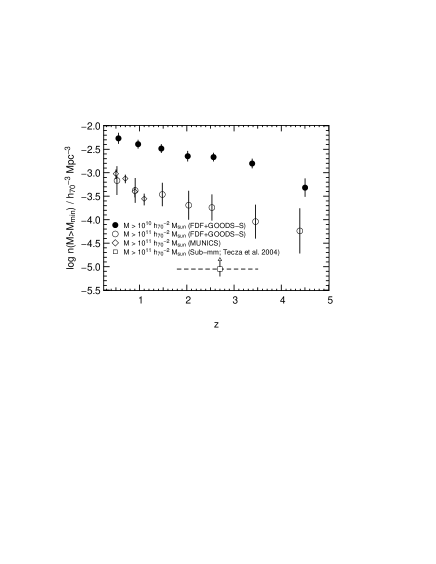
Figure 4.— The number density of galaxies with stellar masses $M>10^{10}\mathrm{M_{\odot}}$ and $M>10^{11}\mathrm{M_{\odot}}$. Results from the MUNICS survey as well as results from Sub-mm studies are also shown.

The fact that the stellar mass densities and the integrated star formation rates give consistent results is encouraging. However, dust-enshrouded starbursts at high redshift would be missing from both the SFR and the MF. However, if the number density of massive sub-mm galaxies derived by Tecza et al. (2004) of $8.9_{-3.3}^{+5.3}\times 10^{-6}\,\mathrm{Mpc}^{-3}$ at $1.8<z<3.6$ is typical of these systems, they do not contribute significantly to the mass density at these redshifts (see below and Fig.4).

Finally, Fig. 4 addresses the number density of massive systems as a function of redshift. We show the numbers of systems with $M>10^{10}\,\mathrm{M_{\odot}}$ and $M>10^{11}\,\mathrm{M_{\odot}}$ as full and open symbols, respectively. The number density of massive sub-mm galaxies estimated by Tecza et al. (2004) is also shown. The most striking features of Fig. 4 is that the number density of the most massive systems shows evolution which is very similar to the evolution of the number density at lower masses over this very large redhsift range. Massive systems are present at all redshifts we probe, their number density decreasing by $0.4\pm 0.2$ dex to $z\sim 1$, by $0.6\pm 0.3$ dex to $z\sim 2$, and by $1\pm 0.45$ dex to $z\sim 4$.

References

- Arnouts et al. (2001) Arnouts, S., et al. 2001, A&A, 379, 740
- Bell et al. (2003) Bell, E. F., McIntosh, D. H., Katz, N., & Weinberg, M. D. 2003, ApJ, submitted
- Brinchmann & Ellis (2000) Brinchmann, J., & Ellis, R. S. 2000, ApJ, 536, L77
- Bruzual & Charlot (2003) Bruzual, G., & Charlot, S. 2003, MNRAS, 344, 1000
- Cohen (2002) Cohen, J. G. 2002, ApJ, 567, 672
- Cole et al. (2001) Cole, S., et al. 2001, MNRAS, 326, 255
- Colless et al. (2001) Colless, M., et al. 2001, MNRAS, 328, 1039
- Dickinson et al. (2003) Dickinson, M., Papovich, C., Ferguson, H. C., & Budavári, T. 2003, ApJ, 587, 25
- Drory et al. (2004) Drory, N., Bender, R., Feulner, G., Hopp, U., Maraston, C., Snigula, J., & Hill, G. J. 2004, ApJ, 608, 742
- Drory et al. (2004) Drory, N., Bender, R., & Hopp, U. 2004, ApJ, 606, L103
- Drory et al. (2001) Drory, N., Bender, R., Snigula, J., Feulner, G., Hopp, U., Maraston, C., Hill, G. J., & de Oliveira, C. M. 2001, ApJ, 562, L111
- Fontana et al. (2003) Fontana, A., et al. 2003, ApJ, 594, L9
- Fontana et al. (2004) Fontana, A., et al. 2004, A&A, 424, 23
- Gabasch et al. (2004a) Gabasch, A., et al. 2004a, A&A, 421, 41
- Gabasch et al. (2004b) Gabasch, A., et al. 2004b, ApJ, 606, L83
- Giavalisco et al. (2004) Giavalisco, M., et al. 2004, ApJ, 600, L93
- Heidt et al. (2003) Heidt, J., et al. 2003, A&A, 398, 49
- Labbé et al. (2003) Labbé, I., et al. 2003, AJ, 125, 1107
- Noll et al. (2004) Noll, S., et al. 2004, A&A, 418, 885
- Rudnick et al. (2003) Rudnick, G., et al. 2003, ApJ, 599, 847
- Schirmer et al. (2003) Schirmer, M., Erben, T., Schneider, P., Pietrzynski, G., Gieren, W., Carpano, S., Micol, A., & Pierfederici, F. 2003, A&A, 407, 869
- Skrutskie et al. (1997) Skrutskie, M. F., et al. 1997, in ASSL Vol. 210: The Impact of Large Scale Near-IR Sky Surveys, 25
- Stasińska et al. (2004) Stasińska, G., Mateus, A., Sodré, L., & Szczerba, R. 2004, A&A, 420, 475
- Steidel et al. (1999) Steidel, C. C., Adelberger, K. L., Giavalisco, M., Dickinson, M., & Pettini, M. 1999, ApJ, 519, 1
- Tecza et al. (2004) Tecza, M., et al. 2004, ApJ, 605, L109
- Tully et al. (1998) Tully, R. B., Pierce, M. J., Huang, J., Saunders, W., Verheijen, M. A. W., & Witchalls, P. L. 1998, AJ, 115, 2264
- York et al. (2000) York, D. G., et al. 2000, AJ, 120, 1579