Transmission of light in deep sea water at the site of the Antares neutrino telescope

Abstract

The ANTARES neutrino telescope is a large photomultiplier array designed to detect neutrino-induced upward-going muons by their Cherenkov radiation. Understanding the absorption and scattering of light in the deep Mediterranean is fundamental to optimising the design and performance of the detector. This paper presents measurements of blue and UV light transmission at the ANTARES site taken between 1997 and 2000. The derived values for the scattering length and the angular distribution of particulate scattering were found to be highly correlated, and results are therefore presented in terms of an absorption length $\lambda_{\mathrm{abs}}$ and an effective scattering length $\lambda_{\mathrm{sct}}^{\mathrm{eff}}$. The values for blue (UV) light are found to be $\lambda_{\mathrm{abs}}\simeq 60(26)$ m, $\lambda_{\mathrm{sct}}^{\mathrm{eff}}\simeq 265(122)$ m, with significant ($\sim$15%) time variability. Finally, the results of ANTARES simulations showing the effect of these water properties on the anticipated performance of the detector are presented.

The ANTARES Collaboration
, , , , , , , , , , , , , , , , , , , , , , , , , , , , , , , , , , , , , , , , , , , , , , , , , , , , , , , , , , , , , , , , , , , , , , , , , , , , , , , , , , , , , , , , , , , , , , , , , , , , , , , , , , , , , , , , , , , , , , , , , , , , , , , , , , , , , , , , , , , , , , , , , , , , , , , , , , , , , , , , , , , , , , , , , , , , , , ,

1 Introduction

The Antares undersea neutrino telescope [1] will use an array of photomultiplier tubes (PMT) in the deep Mediterranean Sea to detect the Cherenkov light emitted by muons resulting from the interaction of high energy neutrinos with matter. The muon track is reconstructed from the arrival time of detected photons. The performance of the detector is therefore critically dependent on the optical properties of sea water, in particular on the velocity of light and on the absorption and scattering cross-sections. All these parameters vary with the photon wavelength. The relevant spectrum spans from ultraviolet to green (see figure 1); the Cherenkov light spectrum varies like $1/\lambda^{2}$, the photomultiplier tube quantum efficiency becomes too low to probe wavelengths longer than $600$ nm, while the glass pressure sphere that surrounds the phototube absorbs the light at wavelengths shorter than $320$ nm. Seasonal variations in sedimentation in the sea water [2] might induce variations in the optical parameters.

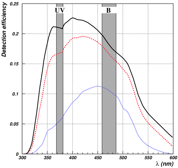
Figure 1: Detection efficiency as a function of wavelength. The solid curve shows the PMT quantum efficiency and the absorption by the glass of the PMT, the optical gel and the protective glass sphere housing the PMT [25]. The dashed and dotted curves are calculated with a path length in water of 5 m and 30 m respectively, assuming a characteristic wavelength dependence of the water absorption length as given in [3]. The effect of scattering is not included. The bands labelled “B” and “UV” indicate the wavelengths at which measurements were undertaken at the Antares site.

Several measurements of sea water attenuation have been performed in the past. The Dumand collaboration reported an attenuation length varying with the light wavelength and reaching a maximum value of 60 m, with 50% accuracy, for a wavelength of 500 nm [4]. The Nestor collaboration measured a similar behaviour. The maximum attenuation length was found at 490 nm and was estimated to be $55\pm 10$ m [5]. The Baïkal experiment found a maximum absorption length of about 20 m for a wavelength of 490 nm [6]. Measurements performed in pure water show that the maximum of the attenuation length is at lower values of the wavelength in this medium ($\sim 400$ nm) [7, 8]. The maximum value was measured around 90 m with 40% accuracy. More recently, measurements of the absorption spectrum in pure water have been reported, with maximum absorption lengths of 160 $\pm$ 15 m at 420 nm [9] and of 225 $\pm$ 30 m at 417 nm [10].

In order to reach an optimal knowledge of the light propagation properties at the detector site all relevant parameters concerning photon absorption and scattering should be measured. These parameters, described in section 3, will be directly measured and continuously monitored by the Antares experiment using an instrumentation line. Until now, the adopted approach has been to measure these parameters with in situ autonomous devices, and these measurements are the subject of this paper. We present time-of-flight distributions of photons emitted from a pulsed isotropic light source and detected by a PMT at different distances from the source and for two wavelengths (blue and UV, as indicated in figure 1). Knowledge of the time-of-flight distribution is essential in order to reconstruct muon tracks. While this approach is not sufficient to fully determine the differential cross section of the photon scattering process, the absorption length can be measured unambiguously. A parameterisation which reproduces the main features of the scattering process can be obtained, sufficient for the needs of the tracking algorithms and of the detector simulation.

2 Experimental setup and measurement procedure

The site chosen for the deployment of the detector is southeast of Toulon ($42^{\circ}50^{\prime}$N $6^{\circ}10^{\prime}$E), 40 km from shore at a depth of 2475 m. During several sea campaigns from 1997 to 2000 we have improved the experimental setup devoted to the study of the light transmission properties, and refined the analysis of the data. We focus, in this section, on the final experimental configuration.

2.1 The mooring line

The measuring system is mounted on an autonomous mooring line anchored by a sinker. The line remains vertical through the flotation provided by syntactic buoys. After deployment, an acoustic modem is used to control the measurement from the surface ship which stays in the vicinity of the zone where the line was sunk. A sketch of the mooring line including information on approximate heights from the sea floor is displayed in figure 2.

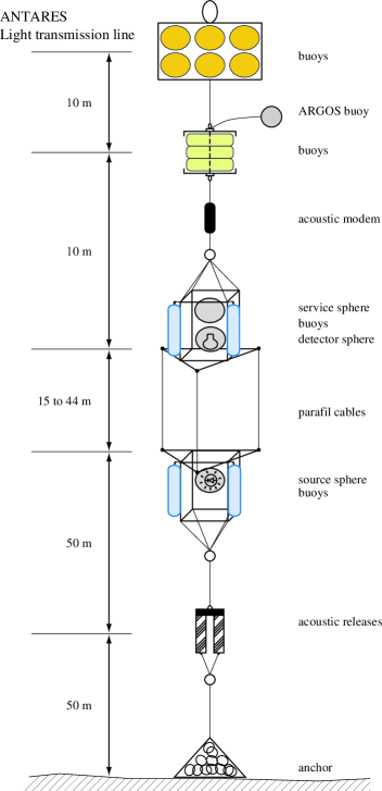
Figure 2: Sketch of the mooring line used for the measurements of the water transmission properties. The figure is not to scale.

The measuring system consists of 17^′′ pressure resistant glass spheres mounted on two triangular aluminum frames. A set of three mechanical cables attached to the vertices of the two frames defines their separation distance. The bottom frame supports a light source sphere which contains a set of LEDs with their pulsers. The top frame supports a detector sphere facing the light source sphere, and a service sphere (cf. figure 5). The detector sphere houses a photomultiplier tube, the DC-DC converter which supplies the high voltage and a pulse height discriminator providing a timing signal for each detected photon. The service sphere contains a TDC, a microprocessor which controls the measurement and records the data, and a set of lithium batteries which power the system. An acoustic modem remote unit is located on top of the measuring system.

2.2 The light source sphere

 

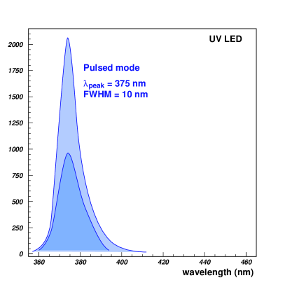
(a) UV LED

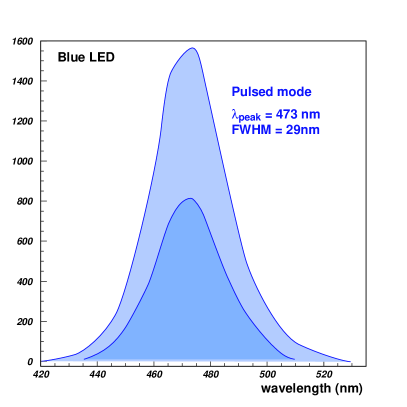
(b) Blue LED

Figure 3: Spectral emission of the blue and UV LEDs (smoothed curves, intensity in arbitrary units). The light and dark areas correspond to the two extreme values of the range of source intensities used for the measurements, with no significant difference in the spectra.

Figure 4: Normalised distributions of photon arrival times measured in air with high statistics for the complete source sphere and with the full setup. Collimators are located between the source and the detector spheres.

In order to obtain an isotropic light source for two wavelengths, 6 pairs of LEDs were mounted on the centres of the faces of a cubic frame 3 cm on a side which also supports the LED pulser boards. Each pair, which includes a blue and a UV LED, is covered with a single 1 cm diameter diffusing cap consisting of glass micro-spheres embedded in epoxy. The cube is installed at the centre of a 17^′′ glass sphere whose external surface has been sand blasted to provide extra diffusion and to remove surface ripples or roughness which can destroy the homogeneity of the emitted light flux. The blue or UV emission colour is chosen for each new acquisition by the operator; all 6 LEDs of the selected colour are then flashed simultaneously.

The spectrum of the light emitted by the LEDs was measured using a spectro-photometre (see figure 3). The peak wavelength and the spectrum FWHM in pulsed mode operation are (375 nm, 10 nm) and (473 nm, 29 nm) respectively for the UV and blue LED. The time distribution of photons emitted by the light source sphere was measured in a dark room for both colours using the complete system (see figure 4) and has a FWHM of about 9 ns, with a tail towards longer times. The isotropy of the source was checked to be within $\pm$12% by measuring the light flux for different orientations of the source sphere with respect to the detector sphere.

2.3 The detector sphere

A small 1^′′ diameter photomultiplier tube glued on the internal surface of a 17^′′ sphere detects photons emitted by the light source. The size of the PMT was chosen in order to limit the counting rate from deep sea optical background. The PMT was then selected for its speed and low transit time spread. Except for the PMT window, the internal surface of the detector sphere is blackened in order to absorb photons outside the PMT detection solid angle.

2.4 The service sphere

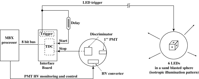
Figure 5: Sketch of the acquisition system.

The service sphere provides a 6 kHz trigger signal which is fed to the LED pulsers and through a delay to a TDC (cf. figure 5). The TDC is started by the delayed trigger signal and stopped by the first PMT signal above the discriminator threshold. The clock of the TDC is defined by a 40 MHz quartz oscillator with each 25 ns period subdivided into 32 approximately equal channels giving an average $\delta t=0.78$ ns time bin. The TDC range can be adjusted by defining its active window; during most of the measurements it was set to 1100 channels in order to accommodate the time distributions for all of the source-detector distances investigated.

The TDC linearity was studied in a dark room by recording a white noise spectrum with high statistics; in the absence of LED flashes, the PMT stop signals were provided by the background created by a controlled light leak. A typical white noise spectrum is displayed in figure 6, showing the non-linearities associated with the 32 channel subdivision pattern. A negative slope in the data is expected, due to the fact that the TDC is single-hit (i.e. stopped by the first PMT signal) and thus cannot record the arrival time of further photons; earlier hits are favoured over later ones. The probability $p_{i}$ that a hit is recorded in bin $i$ given a flat distribution of arrival time is (to first order) $p_{i}=R\;\delta t\times(1-R\;\delta t)^{(i-1)}\simeq R\;\delta t\times[1-(i-1)\;R\;\delta t]$ where $R$ is the rate of background noise.

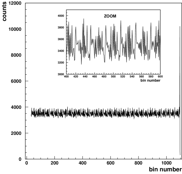
Figure 6: White noise time distribution for TDC calibration. In the enlargement, the non-linearities of the TDC are seen. Given their high noise level, the first (not shown) and last few bins were not used for the recording of physics data.

2.5 Experimental procedure

The cable lengths are set on board for the desired source-detector distance (ranging from 15 to 44 m). Two cable lengths are typically used for each choice of LED voltage.

After the line has reached the sea bed, the acoustic link is established from the surface ship. The light intensity is adjusted via the voltage on the LED pulsers to give a detection efficiency of about 1 detected photon per 100 triggers for the shortest source-detector distance. This ensures that the PMT is working close to the single photoelectron regime. The detection efficiency can artificially increase because of intermittent luminescence bursts. The same intensity is then used for the longer distance. The discriminator threshold is set at a pulse height value of 0.3 times the amplitude of the single-photoelectron peak, in the valley between the peak and the noise. For a given source-detector distance, several data sets corresponding typically to 5$\times$10⁶ triggers each were collected for each of the two light colours. The overall time needed to perform the measurements at one source-detector distance including the drop and recovery of the line is approximately 4 hours.

The various measurements of the water optical properties at the Antares site from 1997 to 2000 are summarised in table 1, in chronological order.

Source	$d_{\rm SD}$	Time of	Comment
	(in m)	year
Blue	6 – 27	Dec. 1997	Different setup (cf. text)
Blue	24, 44	July 1998	2 source intensities
Blue	24, 44	March 1999	standard
UV	15, 24	July 1999	standard
UV	24, 44	Sept. 1999	standard
Blue, UV	24, 44	June 2000	standard
Blue, UV	24	June 2000	400 m above the sea bed

Table 1: Data recorded for the study of the water light transmission properties. The standard configuration is: measurement of the arrival time distribution of photons from a pulsed isotropic source, one source intensity (same for the two source-detector distances $d_{\rm SD}$), source sphere located 100 m above the sea bed (figure 2).

The July 1998 data taken with two source intensities I1 and I2 are used to study the systematics coming from the shape of the source time distribution, which exhibits a slight dependence on the LED pulser voltage (16.5 V in the first case, 18 V in the second). The data recorded 400 m above the sea bed (June 2000) were compared to the other data recorded at 100 m above sea bed to check the water transparency dependence over this depth range, corresponding to the instrumented range of the Antares detector.

Figure 7: Time distributions in UV light for the two source-detector distances (24 and 44 m) of the first June 2000 immersion. Y-axis is proportional to the number of photons collected. The 24 m distribution is normalised to unity. The 44 m distribution is normalised with respect to the one at 24 m, in addition to a $(44/24)^{2}$ factor, so the difference between the two peaks is entirely due to the exponential attenuation factor.

Figure 8: Photon arrival times for a collimated air time distribution and for two distributions taken in situ, with source-detector distances of 24 m and 44 m. All distributions are normalised to unity at the peak. Top panel: June 2000 blue data. Bottom panel: June 2000 UV data. The origin of the time delay axis is set to 0 for direct photons.

As illustrated in figure 8, all the time distributions recorded (1998 to 2000) exhibit a small tail of delayed photons. This corresponds to a small contribution due to scattering between the source and the detector. Figure 8 illustrates, for June 2000 standard blue and UV data, the shape of the photon arrival time distribution in air (no scattering), and in water with a source-detector distance $d_{\rm SD}=24$ m or $d_{\rm SD}=44$ m. Clearly, the width of the main peak comes mostly from time resolution of the setup. The FWHM of spectra recorded for a source-detector distance of 24 m is about 10 ns, to be compared with the intrinsic FWHM of 9 ns of the light source. As expected, the scattering tail increases with a larger separation between the source and the detector. Scattering is also seen to be more significant in UV than in blue: slightly larger increase of the width of the peak region and higher scattering tail, in particular at a distance of 44 m.

The setup deployed for the first immersion (December 1997) was different from the one described above. An $8^{\prime\prime}$ photomultiplier tube is located at a variable distance (6 to 27 m) from a collimated continuous blue LED source ($\lambda=466$ nm). Only the integrated intensity was recorded. The analysis of the data from this immersion is described in section 4.3. All subsequent immersions were done with the setup described in sections 2.1 to 2.4.

3 Simulation of the experiment

The photon propagation (hence the time distribution of photons at a distance $R$ from the source) is governed by the following inherent optical parameters: group velocity of light in the medium $v_{g}$, absorption length $\lambda_{\rm abs}$, and volume scattering function $\beta(\theta)=\widetilde{\beta}(\theta)/\lambda_{\rm sct}$ with units $\rm m^{-1}\cdot sr^{-1}$ (where $\widetilde{\beta}(\theta)$ is the normalised scattering angle distribution and $\lambda_{\rm sct}$ the scattering length). The scattering function is roughly described by the scattering length $\lambda_{\rm sct}$ and the average cosine of the scattering angle distribution (or asymmetry parameter) $\langle\cos\theta\rangle=2\pi\int\widetilde{\beta}(\theta)\,\cos\theta\,d(\cos\theta)$, under the assumption of a specific shape of the scattering angle distribution.

3.1 Physics of propagation of light in sea water

For an isotropic source of photons with intensity $I_{0}$, the intensity $I$ detected at a distance $R$ from the source by a PMT with an active area $A$ is

$$I=I_{0}\frac{A}{4\pi R^{2}}e^{-R/\lambda_{\rm att}^{\rm eff}}\;,$$ (1)

where $\lambda_{\rm att}^{\rm eff}$ is the effective attenuation length, extracted from the total number of photons (i.e. from the integrated time distributions) recorded for two source-detector distances.

An approximate degeneracy reduces the number of parameters needed to characterise the time distribution of photons at a distance $R$ from the source. In particular, strong correlations can be expected if trying to extract $\langle\cos\theta\rangle$ and $\lambda_{\rm sct}$ separately, while $\lambda_{\rm sct}^{\rm eff}$, defined as

$$\lambda_{\rm sct}^{\rm eff}\equiv\frac{\lambda_{\rm sct}}{1-\langle\cos\theta\rangle}\;,$$ (2)

describes the main part of the scattering.

We describe the scattering angle distribution following the approach of Morel and Loisel [12]: the scattering angle distribution is expressed as the weighted sum of molecular and particulate scattering. The molecular scattering is described by the Einstein-Smoluchowski formula for pure water,

$$\widetilde{\beta^{m}}(\cos\theta)=0.06225\;(1+0.835\cos^{2}\theta)\;,$$ (3)

which is reminiscent of the form

$$\widetilde{\beta^{\rm Ray}}(\cos\theta)=\frac{3}{16\pi}\;(1+\cos^{2}\theta)\;,$$ (4)

commonly called Rayleigh scattering. The 0.835 factor (rather than 1) is attributable to the anisotropy of the water molecules. The particulate scattering is described by the Mobley et al. [13] tabulated distribution $\widetilde{\beta^{p}}(\cos\theta)$, obtained by averaging the similar particulate angle distributions measured by Petzold in very different seas [14], at a wavelength of $514$ nm.

The total normalised scattering angle distribution is of the form:

$$\widetilde{\beta}(\cos\theta)=\eta\widetilde{\beta^{m}}(\cos\theta)+(1-\eta)\widetilde{\beta^{p}}(\cos\theta)\;,$$ (5)

with $\eta$ the ratio of molecular to total scattering. The average cosine of the total scattering angular distribution is

$$\langle\cos\theta\rangle=(1-\eta)\times\langle\cos\theta\rangle^{p}=(1-\eta)\times 0.924\;,$$ (6)

since the average cosine of Petzold’s distribution is 0.924. In natural waters, $\eta$ is typically less than 0.2 [12], so $\langle\cos\theta\rangle$ is large and the use of equation 2 is justified.

3.2 The Monte Carlo simulation

A detailed Monte Carlo simulation, which includes the geometry of the experimental setup and the optical properties of the medium, has been used to analyze the experimental time distributions and extract the light transmission parameters at the Antares site. The parameters of the Monte Carlo are the absorption length $\lambda_{\rm abs}$, the scattering length $\lambda_{\rm sct}$, the fraction $\eta$ of molecular scattering, the source-detector distances $d_{i}$, the origin of time for each distribution (or the time $t_{i}$ at which direct photons reach the detector located at a distance $d_{i}$ from the source) and the collection efficiency for each distribution.

For each photon, the distance $x$ it will travel before being absorbed is selected randomly from the probability distribution proportional to $\exp(-x/\lambda_{\rm abs})$. The photon’s distance to its first scattering is similarly selected according to $\exp(-x/\lambda_{\rm sct})$. If the absorption distance is shorter, the photon is propagated to its point of absorption and stopped. Otherwise, the type of scattering (molecular or particulate) is selected according to their respective probabilities $\eta$ and $1-\eta$; the photon is propagated to its point of scattering where a new photon direction is sampled from the appropriate angular distribution and a new scattering distance is drawn. This is repeated until the total length of the photon path reaches its absorption distance. Time distribution histograms are filled whenever the photon reaches a radial distance from the source corresponding to one of the possible source-detector separations. Weights are applied to take into account the dependence of the PMT detection efficiency on the angle of incidence of the photon on the photocathode [15] or to study a possible anisotropy of the source emission. Each Monte Carlo distribution results from the propagation of one million photons.

The time distribution of the emitted light pulse is taken from the one measured in air for direct photons (see figure 4), its angular distribution is taken as isotropic, and its spectrum as monochromatic (see actual spectral width in figure 3) at its central wavelength.

The obtained Monte Carlo photon spectrum corresponds to a light source with a vanishingly small intensity, dominated by single photon events. For realistic intensity conditions, since the TDC is working in the single hit mode, one needs to correct the spectrum for multi-photon events where the first one only is detected. This correction depends on the average rate of detection per light pulse trigger, and is calculated assuming Poisson statistics. The background is removed from the data spectra (see section 4.1 on the data processing) so Monte Carlo spectra are generated with no noise.

4 Data analysis

4.1 Data processing

For each immersion, several data sets were taken with the same configuration. They are all fully compatible and proved the excellent reproducibility of the data over a period of a few hours. They are therefore combined to reduce the statistical noise on the data.

Each recorded time distribution histogram is first corrected for the non-linearity of the TDC with a bin by bin division by a slope-corrected white noise time distribution (cf. section 2.4) as shown in figure 6.

The optical background at this site was studied in detail [16]. It consists of a variable bioluminescence component superimposed on a constant component due to the radioactive decay of ⁴⁰K. During periods without bioluminescence bursts, it exhibits a rate $\widetilde{R}$ of about 0.1 kHz/cm², contributing as a constant component in the time distribution through random stop signals. Bioluminescence bursts can reach rates $\widetilde{R}$ up to several tens of kHz/cm² generally lasting for hundreds of micro-seconds to seconds i.e. for longer than the time range of the TDC. Given the highest rates observed, bioluminescence bursts only contribute as an additional noise which appears as a linearly decreasing component. Extrapolating the result of section 2.4, the total number of background events $N_{i}$ in bin $i$ of the spectrum in the region free of LED events is therefore given by

$$N_{i} = \sum_{j=1}^{N_{\rm triggers}}R_{j}\;\delta t\;[1-(i-1)R_{j}\;\delta t]$$ (7)

$$= \left(\sum_{j=1}^{N_{\rm triggers}}R_{j}\;\delta t\right)-(i-1)\left(\sum_{j=1}^{N_{\rm triggers}}(R_{j}\;\delta t)^{2}\right)$$

$$= a-(i-1)b\;,$$

where $N_{\rm triggers}$ is the number of triggers and $R_{j}$ is the background rate (from bioluminescence and the decay of ⁴⁰K) during cycle $j$ on the $1^{\prime\prime}$ PMT ($R=\widetilde{R}S$). The background contribution is determined by a first-order polynomial fit to the data in the region free of LED hits (i.e. before the signal from the LED direct photons): $N_{i}=a-(i-1)b$. Over 500 bins are available for the noise fit. The background rates were seen to vary between 0.2 and 2.5 kHz/cm².

When taking into account the fact that the multi-hit correction applies to the sum of the hits from the background noise and from the LED source, the background to be subtracted from each bin $i$ of the data is given by the following equation (which results from the difference between the expected distributions in the presence and in the absence of noise):

$$N_{\rm noise}(i) = \sum_{j=1}^{N_{\rm triggers}}\left[(R_{j}\;\delta t+R_{{\rm LED}_{i}}\;\delta t)\left(1-(i-1)R_{j}\;\delta t-\sum_{k=1}^{i-1}R_{{\rm LED}_{k}}\;\delta t\right)\right]$$ (8)

$$-N_{\rm triggers}\times R_{{\rm LED}_{i}}\;\delta t\left(1-\sum_{k=1}^{i-1}R_{{\rm LED}_{k}}\;\delta t\right)$$

$$= a-(i-1)b-a\sum_{k=1}^{i-1}R_{{\rm LED}_{k}}\;\delta t-(i-1)\;a\;R_{{\rm LED}_{i}}\;\delta t$$

where $a$ and $b$ are the same as in equation 7 and $R_{{\rm LED}_{i}}$ is the rate of hits in bin $i$ coming from the LED source (independent of the cycle number). Three correcting terms to the canonical value $a$ of the background appear in equation 8. The slope $b$ in the noise remained small ($b<10^{-3}$). The intensity of the source was chosen so as to minimise the multi-hit correction (and maintain a reasonable signal-to-noise ratio), so that $\sum_{k=1}^{i-1}(R_{{\rm LED}_{k}}\;\delta t)$ is at most $\sim 5\%$ and the second correcting term also remains small. The last term, however, can be quite large in bins where the rate of hits from the LED source is large.

The result of this procedure is illustrated in figure 9 with the example of blue data taken in June 2000.

Figure 9: Noise counts subtracted from the blue data of June 2000. The thin solid line is the level the noise would have had in the absence of LED hits.

The spectrum results from a total of $6\times 10^{6}$ triggers, with an average collection efficiency of 6%. The noise level estimated from the first 700 bins is $a=6.05$ with a slope $b=-8.3\times 10^{-5}$. Bin number 750 contains the highest signal, with 3335 counts and a noise contribution of $-9$ hits, meaning that the photons collected earlier in the spectrum prevented 9 signal counts from reaching this bin. The noise level in the tail of the spectrum is stable at a level of 5.6 counts.

After the subtraction of the background, when two different source-detector distances are available for the same date and source intensity, a measure of the effective attenuation length is obtained from the integrated time distributions (cf. section 4.3). The experimental time distributions are then fitted simultaneously to Monte Carlo distributions to extract the absorption and scattering parameters (cf. section 4.4).

4.2 Group velocity of light

The group velocity of light can be computed from the equation

$$v_{g}=\frac{c}{n}\times\left(1+\frac{dn/n}{d\lambda/\lambda}\right)\;,$$ (9)

using various empirical models for the index of refraction $n$ evaluated for the parameters of the Antares site (pressure $p=230$ atm, salinity $S=38.44\,^{\circ}\!/\!_{\circ\circ}$ and temperature $T=13.2^{\circ}\rm C$).

Using four different experimental data sets of pure water and sea water under various pressures, Millard and Seaver [17] (thereafter referred to as MS) have developed a 27-term algorithm that gives the index of refraction to part-per-million accuracy over most of the oceanographic parameter range (salinity $S=0-40\,^{\circ}\!/\!_{\circ\circ}$, temperature $T=0-30^{\circ}\rm C$ and pressure $p=1-1080$ atm), but only over a limited range of wavelengths ($500-700$ nm) so that we need to extrapolate to use it for our wavelengths of 375 and 473 nm. The result is illustrated in figure 10, curve labelled MS.

A simple empirical equation for the index of refraction of sea water $n(\lambda,S,T)$ for $\lambda$ in $[400-700]$ nm can also be found in [18] by Quan and Fry (thereafter referred to as QF), based on data from Austin and Halikas [19]. The pressure dependence was not included in their equation, so we added it assuming the same linear dependence as that observed on pressure-temperature plots from [20]. The wavelength dependence of this model is the curve labelled QF in figure 10, showing excellent compatibility with the MS model.

As an experimental verification, the following consistency check was performed. From the time distributions recorded with two source-detector distances for a unique source intensity, one can extract the group velocity of light $v_{g}=\Delta d/\Delta t$ where $\Delta d$ is the difference between the source-detector distances for the two immersions, and $\Delta t$ is the difference between the times at which the non-scattered photons emitted by the source reach the detectors located at the two distances from the source.

A length difference $\Delta d=20.60\pm 0.14$ m was measured on shore under a tension of 50 kg on the cables to simulate the buoyancy pull of the immersed line. The time differences are

$$\Delta t=\left\{\begin{array}[]{lc}94.3\pm 0.1\;({\rm stat.})\pm 0.1\;({\rm syst.})\;{\rm ns}&({\rm Blue})\\ 95.7\pm 0.1\;({\rm stat.})\pm 0.1\;({\rm syst.})\;{\rm ns}&({\rm UV})\end{array}\right.\;,$$ (10)

where the first error is the statistical error and the second a systematic error coming from the measurement of the electrical length of the electric cables joining the source to the detector (a cable was associated with each source-detector distance). These data therefore imply the following velocities of light (the error includes the uncertainties on $\Delta d$ and $\Delta t$ stated above), also plotted in figure 10:

$$v_{g}\;({\rm experimental})=\left\{\begin{array}[]{lc}0.2185\pm 0.0015\;{\rm m/ns}&({\rm Blue})\\ 0.2153\pm 0.0015\;{\rm m/ns}&({\rm UV})\end{array}\right.\;.$$ (11)

Figure 10: Comparison of measurements of the group velocity of light with model predictions, for $\lambda=472.5$ nm (Blue) and $\lambda=374.5$ nm (UV). The phase velocity as a function of wavelength is also shown.

As can be seen from the figure, experimental and analytical values are in good agreement. Given the large uncertainty on the determination from the data of the group velocity of light, however, the value of $v_{g}$ in the Monte Carlo is set to the average of the analytical estimates described above, i.e.:

$$v_{g}\;({\rm model})=\left\{\begin{array}[]{lc}0.2178\;{\rm m/ns}&({\rm Blue})\\ 0.2134\;{\rm m/ns}&({\rm UV})\end{array}\right.\;.$$ (12)

It should be noted that the results of the Monte Carlo fit are not influenced by a small change in the chosen value of the group velocity.

4.3 Effective attenuation length

The effective attenuation length $\lambda_{\rm att}^{\rm eff}$ gives an indication of the fraction of the photons emitted by the source that are detected (including those that reach the detector although they have scattered on their way). It varies with the angular distribution of the source emission and with the angular acceptance of the detector. It can be computed from the ratio of the total light detected at the two source-detector distances $d_{1}$ and $d_{2}$:

$$\frac{\int N_{d_{1}}(t)\;dt}{\int N_{d_{2}}(t)\;dt}=\frac{d_{2}^{2}}{d_{1}^{2}}\times\exp\left(-\frac{d_{1}-d_{2}}{\lambda_{\rm att}^{\rm eff}}\right)$$ (13)

where $N_{d_{i}}(t)$ is the time distribution at distance $d_{i}$ after background subtraction and multi-photon event correction. The effective attenuation lengths and the corresponding statistical errors for the data listed in table 1 are given in tables 3 and  3.

An uncertainty in the noise subtraction procedure would not affect this result, as explained in section 4.5.2. The two data sets taken in July 1998 with different LED intensities yield compatible values of the effective attenuation lengths ($62.6\pm 1.0$ m and $60.3\pm 0.4$ m), despite a large correction for multi-photon events in the second case.

As stated in section 2.5, the effective attenuation length was also measured for the different setup deployed in December 1997, which used a continuous collimated source. While the distance $D$ between the source and the PMT was varied from 6 to 27 m, the intensity of the source $\Phi_{\rm LED}$ was adjusted so as to yield a constant current $I_{\rm PMT}$ on the PMT. The setup was calibrated with a similar procedure in air. The emitted and detected intensities in water are related by

$$I_{\rm PMT}\propto\frac{\Phi_{\rm LED}}{D^{2}}\times{\rm exp}\left(-\frac{D}{\lambda_{\rm att}^{\rm eff}}\right)\;,$$ (14)

making it possible to estimate the effective attenuation length from the dependence of the required LED intensity with the distance (cf. figure 11). The agreement of the data with a decrease as given in equation 14 yields an effective attenuation length

$$\lambda_{\rm att}^{\rm eff}\;({\rm Blue,\>collimated})=41\pm 1\;({\rm stat.})\pm 1\;({\rm syst.})\>{\rm m}\;.$$ (15)

The collimation of the source prevents a direct comparison with values given in table 3. A Monte Carlo simulation describing the two setups shows, however, that the above $\lambda_{\rm att}^{\rm eff}$ would yield $\lambda_{\rm att}^{\rm eff}=44\pm 1\;({\rm stat.})\pm 1\;({\rm syst.})$ m with the present (isotropic) setup, similar to the result found in June 2000.

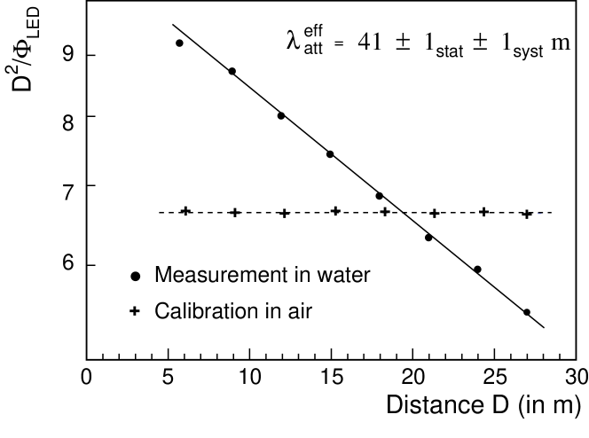
Figure 11: Determination of the effective attenuation length from the setup immersed in December 1997 (see equation 14).

4.4 Absorption and scattering lengths

The uncertainty on the exact cable lengths strongly affects the time of arrival of direct photons, but has a negligible effect both on the shape and on the amplitude of the time distributions. The source-detector distances $d_{1}$ and $d_{2}$ are therefore fixed to the values measured on shore under a tension of 50 kg, while the direct photons arrival times $t_{1}$ and $t_{2}$ are unconstrained to absorb the uncertainties on the distances and avoid biasing the results. The group velocity of light is taken from equation 12. The other free parameters of the fit are the absorption length $\lambda_{\rm abs}$, the fraction of molecular to total scattering $\eta$ (or equivalently $\langle\cos\theta\rangle$ as explained in equation 6) and the effective scattering length $\lambda_{\rm sct}^{\rm eff}$.

All the results are summarised in tables 3 and 3, and plotted in figure 12. The parameters $\lambda_{\rm abs}$, $\lambda_{\rm sct}^{\rm eff}$ and $\eta$ result from the global fit described above. The effective attenuation length $\lambda_{\rm att}^{\rm eff}$ is computed according to the method described in the previous section. Therefore, the usual equality between $1/\lambda_{\rm att}^{\rm eff}$ and the sum of the inverses of $\lambda_{\rm abs}$ and $\lambda_{\rm sct}^{\rm eff}$ does not hold, as they were derived from different methods. The scattering length $\lambda_{\rm sct}$ is obtained from $\lambda_{\rm sct}^{\rm eff}$ and $\eta$ according to equations 2 and 6.

The March 99 data were recorded with a low source intensity, and thus a low collection efficiency, resulting in a high statistical error on the measured parameters. The data sets with two different light intensities available for the July 1998 immersion yield fully consistent results (to within $1\sigma$) for the fit parameters. Only the mean values are therefore reported here.

Epoch	$\lambda_{\rm att}^{\rm eff}$ (in m)	$\lambda_{\rm abs}$ (in m)	$\lambda_{\rm sct}^{\rm eff}$ (in m)	$\eta$	$\lambda_{\rm sct}$ (in m)
July 1998	$60.6\pm 0.4$	$68.6\pm 1.3$	$265\pm 4$	$0.17\pm 0.02$	$62\pm 6$
March 1999	$51.9\pm 0.7$	$61.2\pm 0.7$	$228\pm 11$	$0.19\pm 0.05$	$58\pm 18$
June 2000	$46.4\pm 1.9$	$49.3\pm 0.3$	$301\pm 3$	$0.05\pm 0.02$	$38\pm 8$

Table 2: Summary of the results for the blue data (statistical error only).

Epoch	$\lambda_{\rm att}^{\rm eff}$ (in m)	$\lambda_{\rm abs}$ (in m)	$\lambda_{\rm sct}^{\rm eff}$ (in m)	$\eta$	$\lambda_{\rm sct}$ (in m)
July 1999	$21.9\pm 0.8$	$23.5\pm 0.1$	$119\pm 2$	$0.16\pm 0.03$	$27\pm 4$
Sept. 1999	$22.8\pm 0.3$	$25.6\pm 0.2$	$113\pm 3$	$0.18\pm 0.01$	$28\pm 1$
June 2000	$26.0\pm 0.5$	$28.9\pm 0.1$	$133\pm 3$	$0.12\pm 0.01$	$24\pm 1$

Table 3: Summary of the results for the UV data (statistical error only).

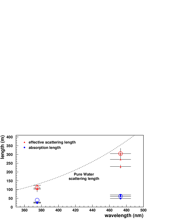
Figure 12: Absorption (dots) and effective scattering (triangles) lengths measured at the Antares site at various epochs for UV and blue data. Horizontal error bars illustrate the source spectral resolution ($\pm 1\sigma$). The large circles are estimates of the absorption and scattering lengths in pure sea water (from [20]). The dashed curve is the scattering length for pure water [21], upper limit on the effective scattering length in sea water.

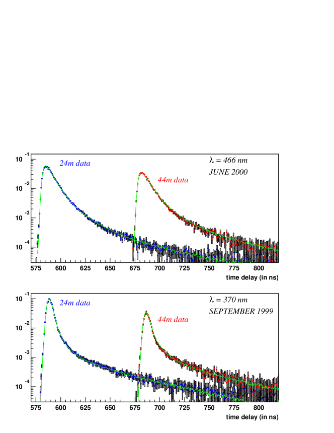
Figure 13: Distributions of photon arrival times with the best-fit Monte Carlo curves superimposed on top of the data. The same normalisation procedure as in figure 8 is applied. Top panel: blue data recorded in June 2000. Bottom panel: UV data recorded in September 1999.

All fit $\chi^{2}$’s per degree of freedom are about 1 (within $\pm 0.5$). Figure 13 illustrates, for June 2000 blue and September 1999 UV data, the photon arrival time distribution in water with a source-detector distance $d_{\rm SD}=24$ m or $d_{\rm SD}=44$ m, with the Monte Carlo fit superimposed on top of the two in-situ distributions.

To illustrate the impact of the water transparency properties at various epochs, time distributions have been generated with each set of best-fit parameters assuming a unique setup, and in particular, a unique choice of the source time distribution: that of the June 2000 UV data. The distributions obtained are shown in figure 14.

Available as a separate figure : scat_art.jpg

Figure 14: Simulated distributions of photon arrival times assuming source-detector distances of 24 and 44 m and the experimental setup of June 2000 UV data , for the best fit parameters of each set of data. The same normalisation procedure as in figure 8 is applied. Top panel: Blue results, bottom panel, UV results.

It can be seen in the figure that the absorption length in UV is smaller than in blue (lower relative height, in UV, of the distribution at the largest distance compared to that at the shortest). The higher tail of delayed photons for the UV distribution is compatible with a smaller scattering length in UV. The UV distributions show little dispersion. The first two blue distributions (July 1998 and March 1999) are quite similar. Only the June 2000 blue distribution differs significantly from the other two, with a much lower tail of delayed photons due to its much larger effective scattering length. Its statistical error bars, however, are also very large, due in particular to the long tail of the time distribution of the June 2000 blue source in the calibration spectrum, which reduces the significance of the tail of delayed photons in the data.

Effective attenuation length results from a combination of absorption and scattering. Since the scattering tail is small (confirmed by the large value of $\lambda_{\rm sct}^{\rm eff}$ compared to $\lambda_{\rm abs}$), the absorption length should be close to the effective attenuation length. As expected, $\lambda_{\rm att}^{\rm eff}\stackrel{{\scriptstyle<}}{{{}_{\sim}}}\lambda_{\rm abs}$ in all data sets. The correlated variations of $\lambda_{\rm att}^{\rm eff}$ and $\lambda_{\rm abs}$ — quantities determined independently and quite robustly — strengthen the hypothesis of fluctuations of the medium optical properties with time.

As explained in section 3.1, $\lambda_{\rm sct}^{\rm eff}$ is used instead of the more physical $\lambda_{\rm sct}$ in order to avoid large ($\sim 80\%$) correlations between $\lambda_{\rm sct}$ and $\eta$. The correlation coefficient between $\lambda_{\rm sct}^{\rm eff}$ and $\eta$ is typically less than $\sim 10\%$. All other correlation coefficients are compatible with zero, confirming the independence of absorption and scattering properties.

Despite the comments of section 3.1, one can try to extract simultaneously the molecular scattering length $\lambda_{\rm sct}^{m}=\lambda_{\rm sct}/\eta$, the particulate scattering length $\lambda_{\rm sct}^{p}=\lambda_{\rm sct}/(1-\eta)$, and the shape of the particulate phase function using a generic one-parameter Henyey-Greenstein function $\widetilde{\beta^{HG}}(g,\cos\theta)$ :

$$\widetilde{\beta^{HG}}(g,\cos\theta)=\frac{1}{4\pi}\;\frac{1-g^{2}}{(1+g^{2}-2g\cos\theta)^{3/2}}\;,$$ (16)

where $g=\langle\cos\theta\rangle$. The results are illustrated with the example of the September 1999 UV data. As expected, a fit with these parameters yields very large correlation coefficients between the various scattering parameters :

$$\left[\begin{array}[]{crrrr}&\lambda_{\rm abs}&\lambda_{\rm sct}^{m}&\lambda_{\rm sct}^{p}&\langle\cos\rangle^{p}\\ \lambda_{\rm abs}&1&-0.19&-0.12&-0.08\\ \lambda_{\rm sct}^{m}&&1&-0.87&-0.96\\ \lambda_{\rm sct}^{p}&&&1&-0.84\\ \langle\cos\rangle^{p}&&&&1\\ \end{array}\right]\,.$$ (17)

The plots of figure 15 show the existence of a $\chi^{2}$ minimum as a function of $\lambda_{\rm sct}^{\rm eff}$, here found for $\lambda_{\rm sct}^{\rm eff}\sim 100$ m, but indicate large degeneracy between $\eta$ and $\langle\cos\theta\rangle$ (region delimited by the dashed line). For instance, the dot and the star shown in these plots have radically different scattering parameters (cf. table 4), although the time distributions for either set of parameters are almost indistinguishable. This follows from identical scattering angle distributions except for small angles (less than $\sim$30 degrees) to which the experiment is poorly sensitive.

dot position			star position
$\lambda_{\rm sct}$	=	$30{\;\rm m}$	$\lambda_{\rm sct}$	=	$76{\;\rm m}$
$\eta$	=	$0.25$	$\eta$	=	$0.56$
$\langle\cos\rangle_{P}$	=	$0.924$	$\langle\cos\rangle_{P}$	=	$0.54$

Table 4: Scattering parameters at two locations of the degeneracy valley indicated with a dot and a star respectively in figure 15.

Available as a separate figure : EtaMcEff_NB.jpg

Figure 15: $\eta$ vs. $\langle\cos\rangle$ for various slices in $\lambda_{\rm sct}^{\rm eff}$. The various shades of grey separate equidistant regions with a difference of 0.5 in the normalised $\chi^{2}$ per degrees of freedom. The dashed line delimits the $1\sigma$ valley. The dot and the star correspond to the scattering parameters in table 4.

This degeneracy in the description of the scattering properties explains the use of the widely cited scattering measurements of Petzold [14] for the particulate scattering phase function, only allowing $\eta$, the fraction of molecular to total scattering, to vary.

4.5 Discussion on systematic uncertainties

Several sources of systematic uncertainties may affect the results of the analysis. These include the slight anisotropy of the source (see section 2.2), an uncertainty in the noise determination (see section 4.1), the reproducibility of the source intensity at a given voltage for the simultaneous fit of time distributions recorded several hours apart (for the two source-detector distances), the knowledge of the time resolution of the source (time distribution in the absence of scattering, measured in the lab, cf. section 2.2) and the angular detection efficiency of the detector module. The systematics that affect the relative normalization of the spectra taken with the two source-detector distances will mostly have an impact on the effective attenuation length and on the absorption length, while those that change the shape of the spectra will rather affect the scattering length. These systematics are studied with the help of the Monte Carlo described in section 3.2. An estimate of their effect is given below.

4.5.1 Source anisotropy

To test the impact of the 12% anisotropy of the source, time distributions are generated with various angular distributions of the light source emission. While the tail of the time distribution is mostly produced by photons having scattered at large angles, the peak (containing most of the hits) comes from photons that have either reached the detector directly or scattered at small angles, i.e. in either case comes from photons emitted by the portion of the source facing the detector. Since the relevant information for the determination of $\lambda_{\rm abs}$ and $\lambda_{\rm att}^{\rm eff}$ is the relative normalization of the time spectra collected with two source-detector distances, which to first order is the relative peak height, and since the source sphere remains in the same position with respect to the detector for all the measurements, the source anisotropy has a negligible impact on the absorption and the effective attenuation lengths. It induces a small distortion on the tail of the time distributions, however, with an impact of the order of 4% on $\lambda_{\rm sct}$ or $\lambda_{\rm sct}^{\rm eff}$.

4.5.2 Noise subtraction

An uncertainty in the noise subtraction will not affect the absorption nor the effective attenuation lengths since the noise remains small compared to the signal, and absorption dominates largely over scattering. On the other hand, the scattering length is mostly determined from the tail of the photon arrival time distribution, which is barely above noise level. The scattering length is therefore crucially dependent on the precision of the noise subtraction. For data taken after June 1999, the spectra have 1100 time bins. The noise contribution before the main signal peak is obtained by a fit over more than 500 bins with negligible impact of the uncertainty on the determination of the noise ($<1\%$). The acquisitions of July 1998 and March 1999, on the other hand, were done with 128 bins only. The noise is therefore estimated from only $\sim 20$ bins in the worst case (data with the short source-detector distance). The uncertainty on the noise determination can then induce an uncertainty on the effective scattering length of at most 8%: 16 m, 13 m and 3 m for the July 1998, March 1999 and June 2000 blue results respectively, and 1 m for all the results in UV.

4.5.3 Stability of LED intensity and PMT efficiency

The LED intensity and the PMT efficiency are stable over a given immersion, as was verified by the excellent reproducibility of time spectra taken under the same conditions up to two hours apart. On two consecutive immersions with different source-detector distances, however, it is not possible to check the stability of the setup. This affects the global normalization of the time spectrum, i.e. the photon collection efficiency (the larger the intensity, the higher the collection efficiency), and thus the effective attenuation length (see section 4.3). Depending on the intensity actually used during each immersion, an assumed uncertainty of 1% on the LED intensity and PMT efficiency affects the effective attenuation length (and similarly the absorption length) by 1 to 11%: 4.5 m, 5.5 m, 1 m and 2 m for the July 1998 (intensity I1), July 1998 (intensity I2), March 1999 and June 2000 blue data respectively, 2 m for the July 1999 and September 1999 UV data and 1 m for the June 2000 UV data. The impact on the scattering length is negligible since the shape of the time spectrum is unchanged.

4.5.4 Source time distribution

The shape of the time distribution of the source varies with the LED input voltage, as illustrated in figure 16. Except for the data recorded in June 2000, time spectra of the source were not always available at the exact same voltage as the one used for the water measurements.

Figure 16: Normalised time spectra of the UV source for DAC voltages of 4.75V (solid curve), 5V (dashed curve) and 5.5V (dotted curve).

Because the relative normalization of spectra at different source-detector distances is independent of the choice of the source intensity, the effective attenuation length, and therefore to first approximation the absorption length, are not affected. The convolution by a slightly different shape of the source spectrum does not affect the level of the scattering tail which is set by the effective scattering length. The latter is therefore also little affected by a poor knowledge of the source time spectrum. The strongest effect appears in the peak of the distribution, and reflects on the angular dependence of scattering, i.e. on the ratio of molecular to particulate scattering. More quantitatively, the data from July 1999 (taken with a DAC voltage of 5.15 V) are fitted with two different source time spectra, first with one at 4.75 V then with one at 5.5 V. The absorption length is unchanged, the effective scattering length increases by 6 m between the two fits and $\eta$ increases by 0.06. Extrapolating these results to the difference between the voltage used under water and the one used for the measurement of the source spectrum yields an uncertainty of 3 m for the July 1998 and March 1999 blue data and of 1.2 m and 2.4 m for the July 1999 and September 1999 UV data respectively. There is no effect on the June 2000 blue or UV results since the same source voltage is used for calibration and data taking.

4.5.5 Angular acceptance of the detector sphere

The angular detection efficiency (studied in [22]) of the glass sphere housing the photomultiplier tube was simulated under the assumption of the exact knowledge of various factors, some of which are affected by large uncertainties as for instance the thickness of the photocathode, the thickness of the optical gel which ensures the optical contact between the photocathode and the glass sphere, or the complex refractive index of the photocathode. The largest changes in the shape of the efficiency curve are obtained by considering the smallest (respectively largest) value of the complex refractive index within its possible range ($1.10+1.70i$ to $2.75+2.50i$), together with the smallest (resp. largest) value of the photocathode thickness (between 16.4 nm and 26.5 nm). Both of these configurations are shown in figure 17.

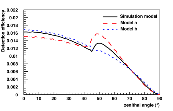
Figure 17: Extreme models of the detector sphere angular efficiency (arbitrary units). The solid curve uses a parameterisation of the Moorhead and Tanner data [15] and is the model used in the simulation of the experimental setup. Model a (resp. model b) uses the thinnest (resp. the thickest) of the photocathodes together with the smallest (resp. the largest) complex refractive index.

From figure 17 it can be seen that a change in the parameters mentioned above reflects upon the ratio $n_{<45^{\circ}}/n_{>45^{\circ}}$ of photons detected at angles smaller or larger than about 45^∘, where the efficiency shows a local enhancement. With model $a$ on the one hand, this ratio decreases, causing more photons to be detected at large angles and therefore requiring a larger scattering length to reproduce the light transmission data. Model $b$ on the other hand requires a shorter scattering length. In both cases, the effect is of the order of 8% on the effective scattering length.

4.5.6 Summary of systematic uncertainties

The total effect of the systematic uncertainties mentioned above is summarised in tables 6 and 6, adding all the systematic errors in quadrature.

Epoch	$\lambda_{\rm att}^{\rm eff}$(in m)	$\lambda_{\rm abs}$ (in m)	$\lambda_{\rm sct}^{\rm eff}$(in m)
July 1998	$60.6\pm 0.4\pm 5$	$68.6\pm 1.3\pm 5$	$265\pm 4\pm 28$
March 1999	$51.9\pm 0.7\pm 1$	$61.2\pm 0.7\pm 1$	$228\pm 11\pm 24$
June 2000	$46.4\pm 1.9\pm 2$	$49.3\pm 0.3\pm 2$	$301\pm 3\pm 27$

Table 5: Summary of the results for the blue data (the first error is the statistical error from table 3, and the second the systematic error).

Epoch	$\lambda_{\rm att}^{\rm eff}$(in m)	$\lambda_{\rm abs}$ (in m)	$\lambda_{\rm sct}^{\rm eff}$(in m)
July 1999	$21.9\pm 0.8\pm 2$	$23.5\pm 0.1\pm 2$	$119\pm 2\pm 10$
Sept. 1999	$22.8\pm 0.3\pm 2$	$25.6\pm 0.2\pm 2$	$113\pm 3\pm 10$
June 2000	$26.0\pm 0.5\pm 1$	$28.9\pm 0.1\pm 1$	$133\pm 3\pm 12$

Table 6: Summary of the results for the UV data (the first error is the statistical error from table 3, and the second the systematic error).

The systematic error is significantly larger than the statistical error. It results in an uncertainty of 5 to 11% on the light transmission parameters. Given these uncertainties, the variations with time of the values of the parameters (cf. section 4.3) are reduced to a $\sim 2\sigma$ effect. To cope with possible temporal variations of the light transmission parameters, which in this paper are shown to be small, the ANTARES detector will monitor continuously the optical properties at the ANTARES site.

4.6 Stability over the line height

During the immersion of June 2000, data were recorded with distances of 100 m and 400 m between the sea bed and the LED source, in both blue and UV, to test for a possible variation of the results with depth. As illustrated in figure 18, the time distributions are fully compatible with one another, whether in blue or in UV, suggesting uniform optical properties along the line height. The $\chi^{2}$ between the measurements at the two heights is 297 for 330 degrees of freedom for the blue data, and 252 for 324 degrees of freedom for the UV data.

 

Available as a separate figure : comp50_350.jpg

(a) Time distributions

(b) Distributions ratios

Figure 18: Comparison of time distributions recorded 100 m above the sea bed (points with grey error boxes in (a)) with the distributions recorded 400 m above the sea bed (overlaying black line in (a)). Top panels: blue data, bottom panels: UV data. The ratio of the distributions, binned into 16 ns bins, are shown in (b).

5 Impact on performance of Antares detector

The primary goal of the Antares detector is to detect high energy muons produced by neutrinos interacting around the detector. In this section, we investigate the extent to which the detection of muons in Antares will be sensitive to the properties of the water (absorption, scattering and angular distribution) and how the uncertainties in the measurement of these properties limit the knowledge of the performance of the detector. Since the effect of scattering on the time distribution is small, scattering is not expected to have a large impact on the reconstruction efficiency, but it might affect the angular resolution.

5.1 Event generation and detector simulation

A sample of $10^{11}$ muon neutrino charged current interactions is generated for neutrinos with an $E^{-1.4}$ spectrum in the energy range 10 GeV $\leq$ $E_{\nu}$ $\leq$ 3 PeV. The angular distribution of the neutrinos is isotropic within the up-going hemisphere. The interaction point is uniformly distributed within a cylinder of 30 km radius centered on the detector and 30 km height enclosing the detector and extending downwards from it. A generator based on LEPTO [23] is used for the neutrino interactions. PROPMU [24] is used for those events starting outside a 200 m cylinder surrounding the instrumented volume of the detector to propagate muons to its surface. Within the 200 m cylinder a full detector simulation is then performed including the effect of using different scattering models for the photon propagation. The Cherenkov light produced by muons and secondary particles is described as a photon field, subsequently converted into a photomultiplier hit probability. A final step simulates the events in the Antares detector. The detector geometry used is described in [25]. The results presented here however are not expected to be strongly dependent on the detector configuration and can therefore be applied to the present configuration [1].

Two parameterisations of the water scattering properties are used. The first uses a combination of molecular scattering and tabulated data from “Petzold” [14] for particle scattering as described in section 3.1. The angular distribution is parameterised by a single parameter $\eta$ (cf. equation 5). Two such models, P1 and P2, are generated with different values of $\lambda_{\rm sct}$ chosen in the range of observed values (see table 7), with P1 illustrating a conservative case. The second parameterisation uses a linear combination of two Henyey-Greenstein angular distributions $\widetilde{\beta^{HG}}(g_{i},\cos\theta)$ to approximate the total scattering angle distribution:

$$\widetilde{\beta}(\cos\theta)=\alpha\,\widetilde{\beta^{HG}}(g_{1},\cos\theta)\,+\,(1-\alpha)\,\widetilde{\beta^{HG}}(g_{2},\cos\theta)\;,$$ (18)

where $\beta^{HG}(g,\cos\theta)$ is given by equation 16. The parameters describing the angular distribution are then $\alpha$ (the relative contribution of the two HG functions), g1 and g2 (the $\left<\cos\theta\right>$ of the two HG functions). Five such models, HG1 to HG5, are generated with different values of $\lambda_{\rm sct}$ and $\left<\cos\theta\right>$.

The simulated models are given in table 7. They have been chosen to include both a set of “reasonable” water properties and extreme cases to probe the maximum effect of each parameter. The numbers quoted for these models are at a wavelength corresponding to the blue LED. The wavelength dependence of the scattering lengths is taken according to the Kopelevich model [20].

Model	$\lambda_{\rm sct}({\rm m})$	$\langle\cos\theta\rangle$	$\lambda^{\rm eff}_{\rm sct}({\rm m})$	$\eta$	$\alpha$	g1	g2
P1	40.8	0.77	175	0.17
P2	52.0	0.77	223	0.17
HG1	52.0	0.77	223		1.000	0.77	0.0
HG2	22.3	0.90	223		1.000	0.90	0.0
HG3	4.4	0.98	223		1.000	0.98	0.0
HG4	40.8	0.90	396		0.985	0.92	-0.6
HG5	52.0	0.90	505		0.985	0.92	-0.6

Table 7: Simulated water models and parameters (for $\lambda=466$ nm).

The scattering angle distributions of all seven models are shown in the upper panel of figure 19. The corresponding time distributions 24 m and 44 m away from the source, as would be measured with the dedicated antares setup (configuration of June 2000 with the blue source), are shown in the lower panel. The variety of time distributions is much larger than that actually observed in the data (see for comparison figure 14).

Available as a separate figure : articleDistrib2.jpg

Figure 19: Top panel: angular distributions $\widetilde{\beta}(\cos\theta)$ for the models P1, P2, HG1 to HG5 described in the text, as well as for pure molecular and pure particulate scattering described in section 3.1 (grey curves). Bottom panel: time distributions for each of the models at source-detector distances of 24 m and 44 m (same normalisation procedure as in figure 8). From top to bottom (better distinction on the second set of curves due to the larger distance of propagation): P1, then P2, then HG1, HG2 and HG3 almost indistinguishable from one another, then HG4 and finally HG5.

Models P1 and P2 include both molecular and particulate contributions to the total scattering angle distribution, the molecular part being a major contributor to the delayed signal, due to its backscattering component which is as significant as its forward scattering one. The two models only differ by their scattering lengths. The smaller scattering length of model P1 therefore generates the larger tail of delayed photons.

Model HG1 reproduces the same $\lambda_{\rm sct}$ and $\left<\cos\theta\right>$ as model P2 but with a different shape for the scattering angular distribution, as illustrated in the upper panel of figure 19. Its lesser backscattering component causes the corresponding time distribution to have less delayed photons. In addition, the peak width is increased. Models HG2 and HG3 have the same $\lambda^{\rm eff}_{\rm sct}$ as model HG1 but with different values of $\left<\cos\theta\right>$, probing the impact of the angular distribution. With HG1, HG2 and HG3 distributions similarly dominated by forward scattering, it is the effective scattering length that governs the levels of the tail of delayed photons. The corresponding time distributions are thus, as expected, almost indistinguishable for the three models. Models HG4 and HG5 have the same $\left<\cos\theta\right>$ as model HG2 but with different $\lambda^{\rm eff}_{\rm sct}$. The angular distribution in models HG4 and HG5 is similar to that of model HG2 with an enhanced backscattering component. The latter is not sufficient however to raise significantly the tail of delayed photons and, as can be expected, the increasing effective scattering lengths lowers the levels of the tail of delayed photons.

The absorption profile is the same in all cases and corresponds to that in [3] normalised to 62.5 m at 470 nm.

Model P2 is the one that best reproduces the experimental results described in the previous sections.

5.2 Event reconstruction and analysis

The three-dimensional reconstruction involves several stages of hit selections to remove PMT hits due to ⁴⁰K noise and bioluminescence, as well as several pre-fits based on plane wave fits through local coincidence and high amplitude hits. The final step is based on a maximum likelihood fit to the distribution of photon arrival times with respect to the expected arrival time of Cherenkov light at a wavelength of 470 nm. The form of the likelihood function is taken from an independent Monte Carlo simulation for muons produced by neutrinos with an $E^{-2}$ spectrum above 1 TeV. That Monte Carlo includes a 55 m effective attenuation length but neglects scattering so there is no initial assumption towards a preferred scattering model. Since the likelihood function is greatly dominated by the peak where the direct photons were expected, the performance of the reconstruction is not strongly affected by the shape of the likelihood function.

The performance of the detector is then defined by two figures of merit of the reconstruction:

Angular resolution $\Delta\alpha$

defined as the median angle between the Monte Carlo neutrino and the reconstructed track.

Effective volume

defined as the fraction of generated events (per bin) which remain after reconstruction and selection, multiplied by the generation volume.

Both of these quantities are defined after selection cuts which eliminate misreconstructed tracks and ensure the purity of the data sample.

5.3 The effect of different water models

The angular resolution as defined above is shown for neutrino energies around 1 TeV ($0.3<E_{\nu}<3$ TeV) and around 100 TeV ($30<E_{\nu}<300$ TeV) for each of the simulated water models in figure 20 as a function of the individual parameters. Several effects contribute to this resolution. The angle between the muon and neutrino at the interaction vertex decreases with increasing neutrino energy. At 1 TeV, this angle is $0.7^{\circ}$ on average [25] and is the most significant contribution to the neutrino angular resolution, whereas at high energies the muon and neutrino are essentially collinear so the accuracy of reconstructing the muon track dominates the angular resolution. The error in the event reconstruction contributes an additional error, bringing the resolution at 1 TeV up to $0.8^{\circ}$. The scattering increases this further to as much as $1.2^{\circ}$, depending on the water model. In the high energy regime, relevant to neutrino astrophysics, the effect of scattering plays a dominant role. For 100 TeV, the average muon-neutrino angle is only $0.04^{\circ}$, the reconstruction brings it up to $0.20^{\circ}$ and the scattering further increases it to as much as $0.53^{\circ}$.

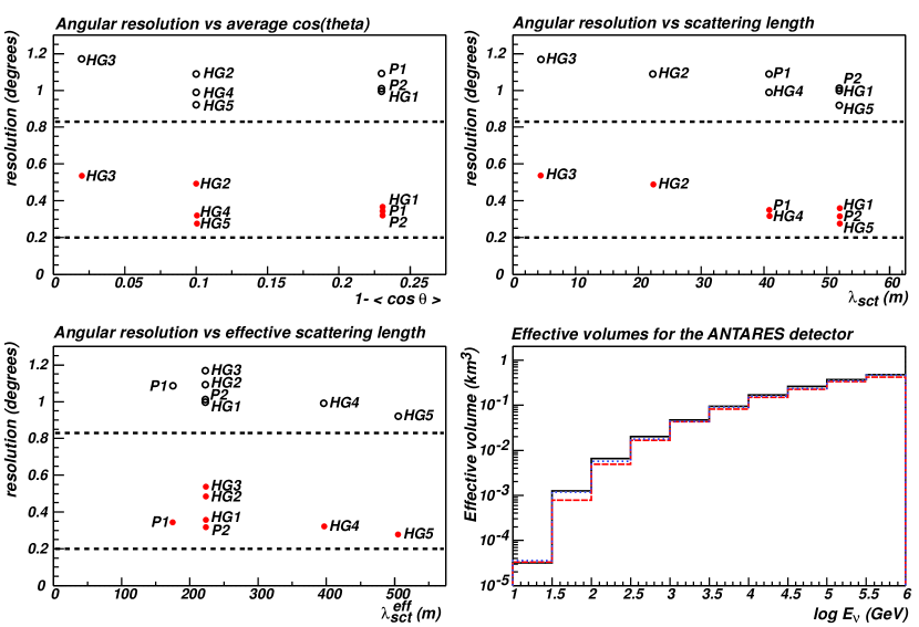
Figure 20: Angular resolution for each of the water models as a function of $1-\left<\cos\theta\right>$, $\lambda_{\rm sct}$ and $\lambda^{\rm eff}_{\rm sct}$. The upper points (open circles) correspond to the neutrino resolution for $0.3<E_{\nu}<3$ TeV with an $E^{-1.4}$ spectrum, the lower points (filled circles) for $30<E_{\nu}<300$ TeV. The horizontal lines show the angular resolution obtained in the absence of scattering in each case. The effective volumes are shown for the two models with the extreme angular resolutions, HG3 (dashed curve) and HG5 (dotted curve) and in the absence of scattering (upper solid curve).

The remarkable agreement between the angular resolutions obtained for models P2 and HG1 implies little sensitivity to the precise shape of the scattering angular distribution. Same $\left<\cos\theta\right>$ and same $\lambda_{\rm sct}^{\rm eff}$ appear to be sufficient to determine the performance of the detector.

The clearest dependence seen in figure 20 is on the scattering length $\lambda_{\rm sct}$. A shorter scattering length degrades the angular resolution. At 1 TeV, the effect of even the most extreme models considered here is at the level of $\pm 12$%. It is at high energies where the differences between the water models in the neutrino angular resolution become most significant, at the level of $\pm 30$% around the central value.

The effective scattering length $\lambda^{\rm eff}_{\rm sct}$ alone is not enough to describe the effect of scattering on the angular resolution, as virtually the full range of angular resolutions obtained are seen for a single effective scattering length of 223 m. Similarly, a wide range of values is seen for a single value of $\left<\cos\theta\right>=0.9$.

Given the results of the in-situ measurements (table 3), we can reasonably estimate $200<\lambda^{\rm eff}_{\rm sct}<400$ m and a $\left<\cos\theta\right>\sim 0.75$ for the blue band. With this assumption, the variation in angular resolution, even at high energy, is at the level of $\pm 10$% around the central value of the angular resolution at $0.32^{\circ}$. Within this, the effect of assuming different angular distributions (with the same $\left<\cos\theta\right>$) gives an uncertainty at the level of $\pm 6$%. Even for the very conservative assumption where $\lambda_{\rm sct}>30$ m, the uncertainty on the angular resolution only increases to 12%.

The variation in the effective volume of the Antares detector over a wide range of neutrino energies between the extreme models is at the level of $\pm 5$%, with models having the worst angular resolutions also yielding the lowest effective volume (see figure 20).

5.4 Angular resolution of the Antares detector

The present design of the Antares detector comprises a 12-string network that will be immersed over the next few years. The event selection can be optimised in terms of angular resolution and effective volume of the detector. The track is obtained by a 2-stage fit: the position and orientation of the PMTs that have been hit are used to obtain points that the track is likely to have crossed. These points are used to obtain an initial track fit. The most probable track is then obtained by the minimization of a function involving the residuals of the times at which the Cherenkov photons emitted along the track reach the PMTs of the detector [26]. In the present stage of the reconstruction software, and considering the scattering model that most closely reproduces the data presented in this paper, model P2 described above, the angular resolution for up-going muon tracks is illustrated in figure 21. For energies $E_{\mu}>300$ GeV the angular resolution for a $E^{-1.4}$ spectrum is

$$\Delta\alpha{\rm(\mu)} = 0.20^{\circ}\pm 0.01^{\circ}\;({\rm stat})\pm 0.02^{\circ}\;({\rm syst})$$ (19)

$$\Delta\alpha{\rm(\nu)} = 0.32^{\circ}\pm 0.02^{\circ}\;({\rm stat})\pm 0.04^{\circ}\;({\rm syst})\>\>.$$ (20)

The systematics are computed from the study presented in the previous section.

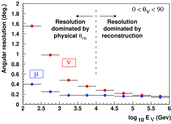
Figure 21: Angular resolution (for scattering model P2) as a function of the neutrino energy for the reconstruction of the muon track (lower curve) or that of the parent neutrino (upper curve) for a 10-string detector.

6 Conclusions

The light transmission at the Antares site has been studied intensively with dedicated setups designed by the collaboration. Absorption and scattering properties of the water for blue light ($\lambda=473$ nm) and UV light ($\lambda=375$ nm) were obtained by measuring the distribution of the arrival times of photons emitted by a pulsed LED source and collected several tens of meters away by a fast photomultiplier tube.

The group velocity of light is found in good agreement with predictions from analytical models. The absorption length is seen to vary slightly in time, with typical values of 60 m in blue and 25 m in UV. These values allow a large effective area ($\sim 0.1\,{\rm km}^{2}$ for neutrino-induced muons with energies in the PeV range) for the planned 12-string Antares detector. With the angular distribution of scattering modelled following the standard approach of oceanographers, the scattering length $\lambda_{\rm sct}$ can be extracted with good confidence from the data, yielding an effective scattering length $\lambda_{\rm sct}^{\rm eff}=\lambda_{\rm sct}/(1-\langle\cos\theta\rangle)$ of $\sim 260$ m in blue and $\sim 120$ m in UV. The various parameters describing the light transmission properties are affected by a 5 to 11% uncertainty, dominated by systematics. Given these large scattering lengths, an angular resolution of $0.3^{\circ}$ should be achieved for $E_{\mu}>300~{}\rm GeV$, according to the present status of the reconstruction software. The uncertainty in the knowledge of the water properties (due for instance to the observed variations) affects our knowledge of the angular resolution and effective volume of the detector by 10% and 5% respectively.

The light transmission properties were checked to be constant at a given time at the two extreme levels (100 m and 400 m above the sea floor) of the active part of a detector line.

The water properties will be monitored with in-situ dedicated instruments during the lifetime of the Antares detector so that the instantaneous values will be available for use in the muon reconstruction software.

References

- [1] E. Aslanides et al. (Antares Collaboration), preprint CPPM-P-1999-02, DAPNIA 99-01, IFIC/99-42, SHEF-HEP/99-06
- [2] Amram, P. et al. (Antares collaboration), Astropart. Phys. 19, 253-267 (2003)
- [3] P.B. Price, Appl. Optics 36 (1997) 1965
- [4] J.R.V. Zaneveld, in Proceedings of the 1980 International DUMAND Symposium, Vol I, V.J. Stenger ed. (Hawaii DUMAND Center, Honolulu, 1981), pp. 1-8
- [5] S.A. Khanaev and A.F. Kuleshov, 2nd NESTOR International Workshop, L.K. Resvanis ed., October 19-21, 1992, pp. 253-269; E.G. Anassontzis, 3nd NESTOR International Workshop, L.K. Resvanis ed., October 19-21, 1993, pp. 614-630
- [6] I.A. Belolaptikov et al, Sixth International Workshop on Neutrino Telescopes, M. Baldo Ceolin ed., Venice, February 22-24, 1994
- [7] T.I. Cuickenden and J.A. Irvin, J. Chem. Phys. 72 (1980) 441
- [8] L.P. Boivin et al, Appl. Opt. 25 (1986) 877
- [9] F.M. Sogandares and S. Fry, Appl. Opt. 36 (1997) 8699
- [10] R.M. Pope and E. S. Fry, Appl. Opt. 36 (1997) 8711
- [11] J.T.O. Kirk, Appl. Opt. 38, 3135 (1999)
- [12] A. Morel and H. Loisel, Appl. Opt. 37, 4765 (1998)
- [13] C.D. Mobley et al., Appl. Opt. 32, 7484 (1993)
- [14] T.J. Petzold, SIO Ref 72-78, Scripts Inst. Oceanogr., La Jolla, 79 (1972)
- [15] M.E. Moorhead and N.W. Tanner, Nucl. Instrum. Meth. A378, 162 (1996)
- [16] Amram, P. et al. (Antares collaboration), Astropart. Phys. 13, 127-136 (2000)
- [17] R.C. Millard and G. Seaver, Deep Sea Res., 37, 121 (1990)
- [18] X. Quan and E. Fry, Appl. Opt. 34, 18 (1995)
- [19] R.W. Austin and G. Halikas, SIO Ref. 76-1, Scripps Inst. Oceanogr., La Jolla, 121 (1976)
- [20] C. D. Mobley, Light and Water (Radiative Transfer in Natural Water), Academic Press (1994)
- [21] A. Morel, chapter 1 in Optical aspects of Oceanography, Academic Press (1974)
- [22] W. H. Schuster, PhD thesis, University of Oxford, (2002), available at http://antares.in2p3.fr/Publications/index.html
- [23] G. Ingelman, A. Edin and J. Rathsman, Comput. Phys. Commun. 101 (1997) 108 [hep-ph/9605286]
- [24] P. Lipari and T. Stanev, Phys. Rev. D 44 (1991) 3543
- [25] Antares proposal, [astro-ph/9907432]
- [26] E. Carmona, 27th International Cosmic Ray Conference (ICRC 2001), 7-15 Aug 2001, Hamburg, Germany