Patchy He II reionization and the physical state of the IGM

Abstract

We present a Monte-Carlo model of He II reionization by QSOs and its effect on the thermal state of the clumpy intergalactic medium (IGM). The model assumes that patchy reionization develops as a result of the discrete distribution of QSOs. It includes various recipes for the propagation of the ionizing photons, and treats photo-heating self-consistently. The model predicts the fraction of He III, the mean temperature in the IGM, and the He II mean optical depth — all as a function of redshift. It also predicts the evolution of the local temperature versus density relation during reionization. Our findings are as follows: The fraction of He III increases gradually until it becomes close to unity at $z\sim 2.8-3.0$. The He II mean optical depth decreases from $\tau\sim 10$ at $z~{}\hbox to0.0pt{\raise 1.72218pt\hbox{$>$}\hss}{\lower 3.01385pt\hbox{$\sim$}}~{}3.5$ to $\tau~{}\hbox to0.0pt{\raise 1.72218pt\hbox{$<$}\hss}{\lower 3.01385pt\hbox{$\sim$}}~{}0.5$ at $z~{}\hbox to0.0pt{\raise 1.72218pt\hbox{$<$}\hss}{\lower 3.01385pt\hbox{$\sim$}}~{}2.5$. The mean temperature rises gradually between $z\sim 4$ and $z\sim 3$ and declines slowly at lower redshifts. The model predicts a flattening of the temperature-density relation with significant increase in the scatter during reionization at $z\sim 3$. Towards the end of reionization the scatter is reduced and a tight relation is re-established. This scatter should be incorporated in the analysis of the Ly$\alpha$ forest at $z~{}\hbox to0.0pt{\raise 1.72218pt\hbox{$<$}\hss}{\lower 3.01385pt\hbox{$\sim$}}~{}3$. Comparison with observational results of the optical depth and the mean temperature at moderate redshifts constrains several key physical parameters.

1 Introduction

The physical properties and the thermal history of the intergalactic-medium (IGM), play an important role in shaping the observed structure in the universe. A proper modelling of the evolution of the IGM is therefore essential for the interpretation of the rapidly accumulating data on the high redshift universe. These data include the secondary temperature and polarization fluctuations in high resolution measurements of the cosmic microwave background (CMB), and absorption features in QSO spectra, which probe the ionized and neutral gaseous components, respectively. Since the distribution of gas follows the underlying mass, these data can be used to constrain the linear mass power spectrum (Croft et al. 1998, 2002; McDonald et al. 2000, 2004; Viel, Haehnelt & Springel 2004).

The gaseous component of the IGM follows, by large, the distribution of the underlying mass distribution of the gravitationally dominant dark matter (DM). The temperature, ionization state and other physical properties are, however, determined by energetic feedback incurred by QSO and galactic activities. This feedback is manifested in photo-ionization and heating of the IGM by radiation emitted by QSOs and galaxies, and in mechanical energy from supernovae explosions of massive stars produce galactic winds that can shock-heat the IGM and enrich it with metals (e.g. Cowie & Songaila 1998; Aracil et al. 2004).

Absorption features in QSO spectra indicate that mechanical energy in galactic winds stirs up the IGM only in the vicinity of galaxies. Observations (Adelberger et al. 2003) have shown that winds can evacuate the neutral hydrogen from within a distance of up to 1-2$\ {\rm h^{-1}Mpc}$ away from Lyman break galaxies (LBGs). Away from galaxies, analysis of the Ly$\alpha$ forest strongly suggests that the moderate density IGM which makes up most of the volume in space, is only affected by ionizing UV photons emitted by QSOs and galaxies.

The gaseous IGM is mainly made of a primordial composition of hydrogen and helium with the former being the dominant element. At $z~{}\hbox to0.0pt{\raise 1.72218pt\hbox{$<$}\hss}{\lower 3.01385pt\hbox{$\sim$}}~{}1000$ these elements recombined and remained neutral until the appearance of stars (and possibly very high redshift QSOs) able to produce sufficient photons to cause significant reionization. Measurement of the polarization anisotropies of the CMB by the Wilkinson Microwave Anisotropy Probe (WMAP) satellite call for an ionized IGM at redshifts as high as $z\sim 17\pm 5$ (Kogut et al. 2003; Spergel et al. 2003). The Gunn-Peterson trough in QSO spectra seems to occur at $z\approx 6$ (Becker et al. 2001; Djorgovski et al. 2001) and might imply a complex reionization history of the IGM with more than a single phase of reionization (Cen 2003; Wyithe & Loeb 2003b). Ionizing radiation from galaxies is also sufficient to singly ionize helium (Benson et al. 2002) at $z>6$. In any case observations of the Ly$\alpha$ forest show that by $z\sim 6$ most of the hydrogen in the universe was photo-ionized and that the IGM is in a quiet state governed by the gravitational drag of the dark matter and the photo-heating of the ionizing radiation (see Rauch 1998 for a review). During this stage a tight relation between the temperature and density is established (e.g. Theuns et al. 1998). The enhancement of QSO activities peaking at $z\sim 2$ is expected to disturb this quiet state by the production of hard photons energetic enough to doubly ionize helium (e.g. Zheng et al. 2004). Modelling double helium reionization is the focus of the current paper. One of our basic assumptions is that QSOs are the main sources for He II reionization at low redshifts. This assumption is sustained by the evidence from observations pointing to He II reionization at redshifts concurrent with the escalation of QSO activities. Although star formation activity also peaks at similar redshifts, radiation from galaxies is too soft to contribute significantly to He II reionization (Benson et al. 2002, Wyithe & Loeb 2003a), unless Population III stars are considered (e.g. Venkatesan, Tumlinson & Shull 2003).

In recent years commendable efforts have been made to observe an He II Gunn-Peterson trough, at the Ly$\alpha$ wavelength of 304Å, in quasar absorption spectra. Estimation of the He II optical depth from the spectrum of the quasars Q0302-003 ($z=3.286$, Dobrzycki et al. 1991; Heap et al. 2000) and of HE 2347-4342 ($z=2.885$, Smette et al. 2002; Zheng et al. 2004) indicate a sharp decline in the optical depth at redshift $z\sim 2.8$. At $z~{}\hbox to0.0pt{\raise 1.72218pt\hbox{$>$}\hss}{\lower 3.01385pt\hbox{$\sim$}}~{}2.8$ the optical depth $\tau~{}\hbox to0.0pt{\raise 1.72218pt\hbox{$>$}\hss}{\lower 3.01385pt\hbox{$\sim$}}~{}4$ and at $z~{}\hbox to0.0pt{\raise 1.72218pt\hbox{$<$}\hss}{\lower 3.01385pt\hbox{$\sim$}}~{}2.7$ the optical depth $\tau~{}\hbox to0.0pt{\raise 1.72218pt\hbox{$<$}\hss}{\lower 3.01385pt\hbox{$\sim$}}~{}1$. This decline implies that He II reionization occurred at $z\sim 3$. The optical depth of the quasar HS 1700+64 ($z=2.743$, Davidsen et al. 1996) $\tau=1.00\pm 0.07$ at redshift $z=2.4$, agrees with the general picture described above. It is important to stress that there may be other explanations for the large fluctuations in the He II optical depth. For example, in Smette et al. (2002), a model is described where optical depth fluctuations along the line of sight are a local effect due to nearby “soft” and “hard” sources, and are unrelated to the global reionization of the IGM.

We aim at a detailed modelling of the state of the IGM during He II reionization. Two approaches can be adopted in achieving this goal. The first is to employ hydrodynamical simulations that include radiative transfer and a good recipe for modelling the distribution of QSOs. An effort towards this goal has been made by Sokasian et al. (2001, 2002) who implemented their radiative transfer numerical code in a cosmological simulation of a box of $67\ {\rm h^{-1}Mpc}$ (run by V. Springel). The simulations offer a valuable insight into the evolution of ionized regions and their topology. The effect of He II reionization on the thermal properties of the IGM have not been modelled in these simulations. This is because radiative transfer is not merged self-consistently with the gas dynamics in the simulations. This is a technical limitation which is expected to be overcome in the near future. However, the simulations are limited by the available CPU power, preventing a thorough exploration of the key physical parameters. The alternative approach is to develop fast semi-analytic models that capture the essential ingredients of the reionization process. This approach has been adopted to study a variety of other problems in structure formation. (e.g. Bi & Davidsen 1997; Kauffmann et al. 1997; Somerville & Primack 1999; Kauffman et al. 1999; Cole et al. 2000; Benson et al. 2001). The basis of semi-analytic models is the synthesis of the knowledge acquired from diverse simulations and analytic reasoning. This synthesis allows us to study a given physical problem with greater detail than individual simulations offer directly. In this paper we propose a Monte-Carlo model for studying He II reionization assuming QSOs are the sole sources of the ionizing radiation. For an assumed cosmology and a form for the QSO luminosity function, the model provides detailed information about the physical state of the IGM. The model is easy to run and allows a thorough exploration of the key physical process. We confront the model with available observational data, and provide predictions for the equation of state of the IGM, i.e., the local temperature-density relation (hereafter ${T-\rho}$ relation). We compare the He II mean optical depth, $\tau(z)$, to the optical depths calculated from the He II Ly$\alpha$ forest of the three quasars mentioned above (Q0302-003, HE 2347-4342 and HS 1700+64) and use this to constrain our model. We also compare the mean temperature, $T(z)$, from our model to the temperatures at the mean density calculated from nine quasars’ Ly$\alpha$ spectra (Schaye et al. 2000) to place further constraints.

The paper is organized as follows. A short theoretical background is presented in § 2. In § 3 we describe our model which we use to investigate the process of patchy He II reionization and its effect on the thermal evolution of the IGM. In § 4 we try to fit observational measurements of the mean temperature and the mean optical depth of the IGM with our model for the power-law $\Lambda\rm{CDM}$ cosmological model implied by the WMAP data (Spergel et al. 2003). We also compute the local temperature-density relation for different redshifts. In § 4.2 we repeat the same computation and comparison for a $\Lambda\rm{CDM}$ model with running spectral index (RSI) (Spergel et al. 2003) and for an open CDM (OCDM) cosmological model. We conclude with a summary and a discussion of the results in § 5.

2 An overview of He II reionization

We assume that double helium reionization is mainly caused by ionizing photons emitted by QSOs, and that the contribution of galaxies is negligible. To justify this assumption we have computed the emission rates of He II ionizing photons from QSOs and galaxies and plotted them in figure 1. The calculation of the emission rate of QSOs is based on that of Madau, Haardt & Rees (1999; hereafter MHR) who performed a similar calculation for hydrogen (see Appendix A). The emission rate of galaxies is estimated using the galform semi-analytic model of galaxy formation. Specifically, we adopt the model and parameters of Benson et al. (2002), except for changes in the cosmological parameters required to match the cosmological model considered here. The reader is referred to that paper, and references therein, for a full description of the model. We choose to ignore the effects of H I reionization on later star formation so as to obtain an upper limit on the number of ionizing photons produced at a given redshift. Note that this model tends to produce more photons than the more recent implementation of the Durham model presented in Baugh et al. (2004; see their Figure 1). As such, we are overestimating the number of ionizing photons produced. We assume that 10% of the produced ionizing photons escape the galaxies into the IGM (observations of low and high redshift galaxies imply escape fractions of  $<$$\sim$ 10%; Leitherer et al. 1995; Tumlinson et al. 1999; Steidel, Pettini & Adelberger 2001). According to figure 1 the emission from QSOs is dominant at redshifts $z\!\!~{}\hbox to0.0pt{\raise 1.72218pt\hbox{$>$}\hss}{\lower 3.01385pt\hbox{$\sim$}}~{}\!1.4$ even if only 20% of the QSOs emission calculated value reaches the IGM.

At some high redshift QSOs begin ionizing He II. The fraction of He III prior to that redshift is assumed to be zero. The mean free path, $l_{\rm ph}$, of an He II ionizing photon is $l_{\rm ph}\sim 0.8n_{\mbox{\scriptsize He\ {\tiny II}},-6}^{-1}{\rm Mpc}$ where $n_{\mbox{\scriptsize He\ {\tiny II}},-6}$ is the physical He II number density in $10^{-6}\rm cm^{-3}$. Initially the mean free path, $l_{\rm ph}$, is much smaller than the mean distance, $d_{\rm QSO}$ between QSOs and so only isolated patches (bubbles) of space are ionized. As the QSO activity increases more photons become available and the volume filling factor of ionized bubbles approaches unity. At this stage, the mean free path in the moderate density IGM, away from discrete absorbers, can exceed the Hubble radius, the radiation field becomes nearly uniform, and an equilibrium between recombinations and photo-ionization is established. This situation is maintained as long as enough photons are produced.

When a given point in the IGM is ionized, its temperature increases by an amount proportional to the fraction of He II. This is a major source of heating in the IGM as each helium atom can be ionized and subsequently recombine several times (Miralda-Escudé & Rees 1994). The dominant cooling mechanism is adiabatic cooling as a result of the cosmic expansion (e.g. Miralda-Escudé & Rees 1994). During the patchy period of ionization large temperature differences between ionized and neutral regions can develop, spoiling any tight relation between the temperature and the density (T-$\rho$) in the IGM (e.g. Theuns et al. 1998). If this period is short lived adiabatic cooling and photo-heating in the later evolution of the IGM work to re-establish the tight T-$\rho$ relation. Much of the thermal history of the IGM at $2<z<5$ is governed by the way He II reionization proceeds.

Figure 1: The QSO and galaxy emission rate of He II ionizing photons per unit comoving volume. For QSOs we plot both the full value and 20% of the emission rate and for three different cosmologies. The solid line is for $\Lambda\rm{CDM}$ with $\Omega_{0}=0.27$, $\Omega_{\Lambda}=0.73$ & $h=0.72$ (Spergel et al. 2003). The dashed line is for the running spectral index model of Spergel et al. (2003) with $\Omega_{0}=0.268$, $\Omega_{\Lambda}=0.732$ & $h=0.71$. The dotted line is for OCDM with $\Omega_{0}=0.3$, $\Omega_{\Lambda}=0$ & $h=0.7$. For galaxies we plot the emission rate with ionizing photons escape fraction of 10% and running spectral index cosmological model.

3 The Monte-Carlo model

Figure 2: Flowchart of the Monte-Carlo method.

Given $N$ random points in the IGM with specified gas density, temperature, and ionization state at some high redshift, $z_{i}$, the model is designed to yield the corresponding quantities at any lower redshift. The model assumes that a uniform ionizing background for hydrogen and singly ionized helium has already been established prior to $z_{i}$. The model aims at following the physical state of the IGM as a result of He II reionization by the QSOs population. At the early stages of He II reionization the mean free path for the absorption of an He II ionizing photon, $l_{\rm ph}$, is short and the reionization proceeds in a patchy way as a result of the discrete distribution of QSOs. At these stages a QSO generates an almost fully ionized bubble as the bounding thin (thickness $l_{\rm ph}$) ionization front propagates outward. The process continues until the QSO fades away. The mean lifetime of a QSO is $\sim 10^{7}$ years (e.g. Hosokawa 2002; Schirber et al. 2004; Porciani et al. 2004) which is much shorter than the recombination timescale (order of 1 Gyr at $z=3$) inside the bubbles. Therefore, we assume that the QSO radiation is emitted in bursts. At later stages when the filling factor of He III regions becomes significant, the mean free path, $l_{\rm ph}$, becomes so large that a non-negligible fraction of the absorbed photons at a given time have actually been produced at significantly larger redshifts. We start the ionization of He II by QSOs at redshift $z_{i}\approx 6$, with hydrogen and helium already singly ionized. We neglect the He II ionization by galaxies. Figure 2 presents a schematic description of the Monte-Carlo model. The details of the model are as follows:

1. Initialization: we work with $N$ points representing random uncorrelated points in the IGM (we use $N=2\times 10^{5}$). At each point we determine the He III abundance fraction, $X$, the temperature, $T$, and the density perturbation, $\delta$. At the initial time, we set $X=0$ for all the points and assign temperatures according to $T=T_{0}(1+\delta)^{2/3}$. At each point, the initial density contrast $\delta_{i}^{\rm in}$ at some very high redshift, $z^{\rm in}=20$, is drawn randomly from a normal (Gaussian) probability distribution function with zero mean and with rms value $\sigma_{0}$.

2. The local density and its evolution: the ionized fraction and the adiabatic cooling/heating depend on the local gas density and its evolution in time. Given the initial mass power spectrum of the dark matter we would like to have a recipe for deriving the gas density contrast as a function of time. Hydrodynamical simulations strongly support the picture in which the gas distribution in the IGM traces the dark matter density smoothed over the comoving Jeans length scale, $x_{\rm J}$, at which pressure forces roughly balance gravity (Hernquist et al. 1996; Theuns et al. 1998). We therefore estimate the gas density power spectrum by smoothing that of the dark matter on the Jeans length scale (see Appendix C for details). We approximate the density contrast $\delta_{i}(z)$ at a point $i$ as follows. The first step is to obtain the gas density variance $\left<\delta^{2}_{i}(z)\right>=\sigma^{2}(z)$ as a function of redshift. Given the linear power spectrum we use the recipe described in Peacock (1999) to derive the corresponding nonlinear power-spectrum. This power-spectrum is then multiplied by an appropriate Jeans smoothing window and integrated to yield $\sigma^{2}$. Let $z^{\rm in}$ be a sufficiently high redshift such that $\sigma^{2}(z^{\rm in})\ll 1$ and such that the QSO emission is negligible at $z^{\rm in}$. Draw a random variable $\delta_{i}^{\rm G}$ from a Gaussian distribution of zero mean and variance $\sigma^{2}(z^{\rm in})$. We write the density contrast, $\delta_{i}(z)$, at any redshift $z<z^{\rm in}$ as

   $$\left(1+\delta_{i}(z)\right)={\rm e}^{\tilde{D}(z)\delta_{i}^{\rm G}+\tilde{D}^{2}(z)b_{0}},$$ (1)

   where the nonlinear growth factor, $\tilde{D}(z)$, is

   $$\tilde{D}(z)=\sqrt{\frac{\ln(1+\sigma^{2}(z))}{\ln(1+\sigma^{2}(z^{\rm in}))}}.$$ (2)

   The form (1) is based on the log-normal model (e.g. Kofman et al. 1994) for the evolution of the density contrast, except that in the standard log-normal model the factor $\tilde{D}$ is replaced with the linear growth factor of density perturbations. The form (2) for $\tilde{D}$ ensures that the variance of $\delta_{i}(z)$ is $\sigma^{2}(z)$ which can be estimated reliably using the recipe outlined below. On can show that $\left<\delta^{2}_{i}(z)\right>=\sigma^{2}(z)$, as follows. If $\delta_{i}^{\rm G}$ is Gaussian, it is easy to see that the mean of $\delta_{i}(z)$ is zero and the variance is $\exp\left[\tilde{D}(z)^{2}\left<(\delta_{i}^{\rm G})^{2}\right>\right]-1$. Hence, using $\left<(\delta_{i}^{\rm G})^{2}\right>=\sigma^{2}(z^{\rm in})\ll 1$ and (2), we find that $\left<\delta^{2}_{i}(z)\right>=\sigma^{2}(z)$. Therefore, the form (1) guarantees a variance of $\sigma^{2}(z)$ for $\delta_{i}(z)$, provided that

   $$b_{0}=-\frac{1}{2}\sigma_{0}^{2}=-\frac{1}{2}\sigma^{2}(z^{\rm in}).$$ (3)

3. The ionization probability: at each time step the ionization state of helium is updated as follows. We assign a probability, $f_{i}$, for photo-ionizing He II at the point $i$, and draw a random number, $p_{i}$, between 0 to 1 from a uniform distribution. If $p_{i}<f_{i}$ then the point $i$ is ionized. We adopt the following form for the photo-ionization probability,

   $$f_{i}=\frac{N_{\rm abs}}{n_{\mbox{\scriptsize He}}}\frac{N\ P_{\rm bias}(\delta_{i})}{\sum_{j=1}^{N}(1-X_{j})(1+\delta_{j})P_{\rm bias}(\delta_{j})},$$ (4)

   where $n_{\mbox{\scriptsize He}}$ is the mean comoving number density of all helium species, $X_{j}$ is the He III abundance fraction in point $j$, and $N_{\rm abs}(z)$ is the total number of ionizing photons per unit comoving volume that are actually absorbed in the current redshift interval $[z(t),z(t+\Delta t)]$ (see below). At the beginning of each time step the number of available ionizing photons is computed as $N_{\rm trs}+\dot{N}_{\rm Q}\Delta t$ where $N_{\rm trs}$ is the number photons that have been transmitted from previous time steps and $\dot{N}_{\rm Q}\Delta t$ is the number of photons that are produced by QSO in the current time steps. The calculation of $\dot{N}_{\rm Q}$ is detailed in Appendix A. The number of available ionizing photons is tabulated in frequency bins and $N_{\rm abs}$ is computed in a self-consistent way as described in Appendix B.

   The factor $P_{\rm bias}$ takes account of the bias between the gas density distribution and the distribution of the He II ionizing photons. At the initial stages of He II reionization, the ionizing photons are preferentially absorbed near the sources. As He II reionization proceeds, the mean free path, $l_{\rm ph}$, becomes large and the ionizing radiation eventually forms a uniform background. In this case the distribution of the ionizing photons is independent of $\delta$. Here we adopt the following form for $P_{\rm bias}$,

   $$P_{\rm bias}(\delta_{i})\propto(1+\delta_{i})^{(b-1)s},$$ (5)

   where $b$ is the bias parameter between the distribution of the QSOs and the gas density field, and $s=s(l_{\rm ph})$ is in general a function of the mean free path, $l_{\rm ph}$, of an He II ionizing photon. We work with three choices for $s(l_{\rm ph})$,

   $$s_{\rm const}=1\;,$$ (6a)

   $$s_{\rm linear}=\left\{\begin{array}[]{cl}x_{\rm J}/l_{\rm ph},&{\rm if}\ l_{\rm ph}>x_{\rm J}\\ 1,&{\rm otherwise}\end{array}\right.\;,$$ (6b)

   and

   $$s_{\rm exp}=\left\{\begin{array}[]{cl}e^{(1-l_{\rm ph}/x_{\rm J})},&{\rm if}\ l_{\rm ph}>x_{\rm J}\\ 1,&{\rm otherwise}\end{array}\right.\;.$$ (6c)

4. He II photo-ionization heating: once a point is flagged for ionization we update its ionized fraction and temperature according to,

   $$X_{i}\longrightarrow 1,$$ (7)

   and

   $$T_{i}\longrightarrow T_{i}+\Delta T(1-X^{\rm prev}_{i}),$$ (8)

   where $\Delta T$ is the increment in the temperature due to photo-ionization heating, and $X^{\rm prev}_{i}$ is the ionization fraction before the current ionization. We also make an attempt at modelling the effect of a finite QSO lifetime, $t_{\rm Q}$, on the reionization process. The model does not contain explicit information on the spatial distribution of the sources. The way we alleviate this problem is by assuming that each freshly ionized point remains ionized for a period of time equal to $t_{\rm Q}$ if it has not been selected for ionization during this time. During this period of time, for each time step, some recombination and photo-ionization heating occur, and can be treated as a local equilibrium.

   The process of drawing random numbers for points continues until all $N_{\rm abs}$ photons are absorbed.

5. He II recombination: recombination reduces the He III abundance fraction by

   $$\frac{{\rm d}X(1+\delta)}{{\rm d}t}=-\alpha_{\mbox{\scriptsize He\ {\tiny II}}}^{(2)}(1+z)^{3}n_{\rm e}X(1+\delta)^{2},$$ (9)

   where $\alpha_{\mbox{\scriptsize He\ {\tiny II}}}^{(2)}$ is the He II case B recombination coefficient (e.g. Verner & Ferland 1996) and $n_{\rm e}$ in the mean comoving number density of electrons.

   At every time step we approximate the reduction in the He III abundance fraction at every point $i$ due to recombination

   $$X_{i}\longrightarrow X_{i}\exp\left[-\alpha_{\mbox{\scriptsize He\ {\tiny II}}}^{(2)}(T_{i})(1+z)^{3}(1+\delta_{i})n_{\rm e}\Delta t\right].$$ (10)

6. Adiabatic cooling/heating: the main cooling process in the moderate density IGM at redshifts $z~{}\hbox to0.0pt{\raise 1.72218pt\hbox{$<$}\hss}{\lower 3.01385pt\hbox{$\sim$}}~{}6$ is adiabatic cooling. The adiabatic cooling/heating is calculated from the thermodynamic dependence between the temperature and density of a monatomic ideal gas

   $$\frac{T}{T_{0}}=\left(\frac{\langle\rho\rangle}{\langle\rho_{0}\rangle}\right)^{2/3},$$ (11)

   where $T_{0}$ and $\langle\rho_{0}\rangle$ are the temperature and the mean density at some initial redshift, $z_{0}$. The mean density, $\langle\rho\rangle\sim(1+z)^{3}$ so that

   $$T=T_{0}\left(\frac{1+z}{1+z_{0}}\right)^{2}\left(\frac{1+\delta}{1+\delta_{0}}\right)^{2/3}.$$ (12)

   Therefore, from equation (12), the adiabatic cooling/heating at every time step is

   $$T_{i}(z) = T_{i}(z+\Delta z)\times$$ (13)

   $$\left(\frac{1+z}{1+z+\Delta z}\right)^{2}\left(\frac{1+\delta_{i}(z)}{1+\delta_{i}(z+\Delta z)}\right)^{2/3}.$$

7. Photo-ionization heating by H I & He I: our basic assumption is that at redshifts $z~{}\hbox to0.0pt{\raise 1.72218pt\hbox{$<$}\hss}{\lower 3.01385pt\hbox{$\sim$}}~{}6$ hydrogen is fully ionized and helium is singly ionized. We also assume a local thermal equilibrium between the background radiation and recombination at every time step. For simplicity we treat He I as extra H I particles, and use the Miralda-Escudé & Rees (1994) analysis for the IGM heating by the H I photo-ionization background radiation, to calculate the temperature increment at every point $i$

   $$T_{i}\longrightarrow T_{i}+\frac{2}{3k}E\alpha_{\mbox{\scriptsize H\ {\tiny I}}}^{(2)}(T_{i})(1+z)^{3}(1+\delta_{i})n_{\rm e}\Delta t,$$ (14)

   where $E$ is the average energy of the absorbed photons minus the average energy lost per recombination, and $\alpha_{\mbox{\scriptsize H\ {\tiny I}}}^{(2)}$ is the H I case B recombination coefficient (e.g. Verner & Ferland 1996).

8. Compton cooling: Compton cooling resulting from free electrons scattering off the CMB photons is non-negligible at redshifts $3<z<6$. This cooling timescale is given by (Peebles 1968)

   $$t_{\rm Compton}=\frac{1161.3(1+X_{e}^{-1})}{(1+z)^{4}[1-T_{0}^{\rm CMB}(1+z)/T_{e}]}{\rm Gyr},$$ (15)

   where $X_{e}$ is the fraction of free electrons, $T_{0}^{\rm CMB}$ is the temperature of the CMB at the present day, and $T_{e}$ is the temperature of the free electrons. At every time step the temperature decrease at every point $i$ due to Compton cooling is

   $$T_{i}\longrightarrow T_{i}-\frac{T_{i}\Delta t}{t_{i}^{\rm Compton}}.$$ (16)

9. Other cooling processes: we have assessed the importance of the following cooling processes: collisional ionization, recombination, dielectronic recombination, collisional excitation, and bremsstrahlung (e.g. Theuns et al. 1998). We have found that all of these processes are negligible for $\delta~{}\hbox to0.0pt{\raise 1.72218pt\hbox{$<$}\hss}{\lower 3.01385pt\hbox{$\sim$}}~{}100$ in the temperature range of interest to us $T~{}\hbox to0.0pt{\raise 1.72218pt\hbox{$<$}\hss}{\lower 3.01385pt\hbox{$\sim$}}~{}10^{5}$K. One should also keep in mind that we assume an instantaneous photo-ionization and photo-heating (equation 7). Rapid energy loss in line excitations and collisional ionization immediately follows and brings the temperature to $T~{}\hbox to0.0pt{\raise 1.72218pt\hbox{$<$}\hss}{\lower 3.01385pt\hbox{$\sim$}}~{}10^{5}\rm K$. This rapid cooling is implicitly included in the temperature increment $\Delta T$ in equation (8). The parameter $\Delta T$ is treated as a free parameter in our model.

3.1 The model input

Table 1: Parameters of the three cosmological models considered here. The parameters of the power-law $\Lambda\rm{CDM}$ and the running spectral index $\Lambda\rm{CDM}$ models are taken from Spergel et al. (2003). The open CDM model has zero dark energy component. The parameters $\Omega_{0}$, $\Omega_{\Lambda}$ and $\Omega_{\rm b}$ are, respectively, the mean density (in units of the critical value) of the of the dark matter, the dark energy (cosmological constant) and the baryon component. The Hubble constant, $h$, in units of $100$ km/s/Mpc, $n$ is the power spectrum power-law, and $\sigma_{8}$ is the rms value of density fluctuations in spheres of radius $8\ {\rm h^{-1}Mpc}$. The spectral index of the RSI model is a function of wavenumber, $k$, and is given by $n(k)=n(k_{0})+[{\rm d}n/{\rm d}\ln k]\ln(k/k_{0})$ with $k_{0}=0.05$ Mpc^-1 and ${\rm d}n/{\rm d}\ln k=-0.031$.

	$\Omega_{0}$	$\Omega_{\Lambda}$	$\Omega_{b}$	$h$	$n$	$\sigma_{8}$
$\Lambda\rm{CDM}$	0.270	0.730	0.0463	0.72	0.99	0.90
RSI	0.268	0.732	0.0444	0.71	Var.	0.84
OCDM	0.300	0.000	0.0463	0.70	1.00	0.90

A basic input of the model are the cosmological parameters. We will present results for three variants of the Cold Dark Matter (CDM) cosmological model. The first is the $\Lambda\rm{CDM}$ cosmological model of a flat universe with a cosmological constant and a power-law power spectrum of density fluctuations. The second is also a $\Lambda\rm{CDM}$ model with similar cosmological parameters but with a running spectral index (RSI) for the power spectrum. The third is an open CDM (OCDM) model, similar to our $\Lambda\rm{CDM}$ model but with no cosmological constant term. The main parameters defining these cosmologies are listed in Table 1. The parameters of the $\Lambda\rm{CDM}$ and RSI cosmologies are taken from the first year WMAP data analysis (Spergel et al. 2003). The OCDM model is not currently viable in view of the WMAP measurements and the observations of Type Ia SNe (e.g. Knop et al. 2003; Riess et al. 2004). Nevertheless, we run our Monte-Carlo model with this cosmological model for the sake of comparison.

Table 2: The input parameters of the Monte-Carlo model: $f_{\dot{N}_{\rm Q}}$ is the QSO emission rate factor, $t_{\rm Q}$ is the mean QSO lifetime, $T_{0}(z\!\!=\!\!6)$ is the initial mean temperature at redshift $z=6$, $\Delta T$ is the temperature increment induced by photo-ionization of He II, $E$ is the cross section weighted excess photon energy for hydrogen ionization, $x_{\rm J}(z\!\!=\!\!3)$ is the comoving Jeans length at redshift $z=3$, $b$ is the QSOs distribution bias parameter, and $s$ is the scaling function between the QSOs and the ionizing emission distributions.

Parameter	Values	Units
$f_{\dot{N}_{\rm Q}}$	0.2, 0.3, 0.4, 0.5, 1.0
$t_{\rm Q}$	0, 5, 10, 20, 40, 60	Myr
$T_{0}(z\!\!=\!\!6)$	1.0, 2.0, 3.0, 4.0, 5.0, 6.0	$10^{4}$K
$\Delta T$	1.0, 1.5, 1.84	$10^{4}$K
$E$	1.27, 2.54, 3.81	$\ {\rm eV}$
$x_{\rm J}(z\!\!=\!\!3)$	0.05, 0.1, 0.2, 0.3, 0.4	$\ {\rm h^{-1}Mpc}$
$b$	1.0, 2.0, 3.0, 5.0, 8.0
$s$	const, linear, exp

The Monte-Carlo model has also to be fed with the input parameters pertaining to the physical processes discussed previously. These parameters are summarized in Table 2. The first parameter in this table, $f_{\dot{N}_{\rm Q}}$, is the QSO emission factor. In Appendix A we describe our calculation of the QSO emission rate of ionizing photons per unit comoving volume, $\dot{N}_{\rm Q}(z)$. The calculation is based on the MHR luminosity function. Although we work with the basic shape of the inferred $\dot{N}_{\rm Q}(z)$ we introduce the factor $f_{\dot{N}_{\rm Q}}$ to allow for an overall reduction in the intensity of emitted radiation. The motivation behind this factor is that several observations and simulations suggest a softer UV radiation field than the standard UV background due to QSOs emission (MHR). Smette et al. (2002) has shown regions of the HE 2347-4342 spectrum in which the He II optical depth is very high and the corresponding H I optical depth is low required photo-ionization by a very soft UV radiation field. Independent evidence is provided by the column density ratios of highly ionized metals ($N_{\rm Si\ IV}/N_{\rm C\ IV}$ versus $N_{\rm Si\ II}/N_{\rm C\ IV}$) at high redshifts (Giroux & Shull 1997; Savaglio et al. 1997; Songaila 1998; Kepner et al. 1999). Numerical simulations of the Ly$\alpha$ forest also suggest a softer UV radiation field (Theuns et al. 1998; Efstathiou et al. 2000).

Next is $t_{\rm Q}$, the mean QSO lifetime. Since the points in the model are not spatially correlated we can take into account the QSOs lifetime only in a very limited way. We assume that a point that was ionized will stay ionized at least for the QSO lifetime. Therefore, $t_{\rm Q}=0$ merely implies that the QSO lifetime is shorter then the model time step.

The mean temperature at redshift $z=6$, $T_{0}(z\!\!=\!\!6)$, is fixed prior to He II reionization. This temperature is set by the interplay between cooling (mainly adiabatic and Compton) and the photo-heating by the hydrogen ionizing background.

The parameter $\Delta T$ is the increment in the temperature due to He II reionization (cf. equation 8). In the limit of a very high ionization fraction an absorbed photon produce only one free electron which loses its energy by Coulomb interactions in the ionized IGM. The temperature increment in this case is given by (Miralda-Escudé & Rees 1994)

$$\Delta T=\frac{2}{3k}X\left(<\!\!\epsilon\!\!>-\ \epsilon_{0}\right)\simeq 1.84\times 10^{4}{\rm K},$$ (17)

where $X=n_{\rm He}/(n_{\rm H}+n_{\rm He}+n_{\rm e})\approx 0.07$ is the fraction of particles which participate in the photo-ionization process from the total number of particles in the gas, $<\!\!\epsilon\!\!>\ \simeq 1.96\times 10^{-10}{\rm erg}$ is the mean energy per photon of photons with energies greater than $4\ {\rm Ry}$ which are emitted by QSOs, and $\epsilon_{0}=4\ {\rm Ry}\simeq 8.72\times 10^{-11}\ {\rm erg}$ is the energy spent per He II ionization.

However, when the ionization fraction is not very high, the electrons produced by photo-ionization may have a large probability of interacting with He I and lose energy in line excitations and collisional ionization. Furthermore, when secondary electrons are produced, the initial energy must be shared among several electrons, and so the final energy per electron is reduced. Therefore, we also explore lower values of $\Delta T$.

The cross section weighted photon energy, $E$, determines the photo-heating due to the H I and He I ionizing photon backgrounds, assuming local equilibrium between the background radiation and the recombination processes (equation 14). Following Miralda-Escudé & Rees (1994) we neglect the temperature dependence of $E$ (which is valid for low temperatures, since the energy lost in recombination is then negligible). In the case of pure hydrogen and for QSOs SED $L(\nu)\propto\nu^{-1.5}$, Miralda-Escudé & Rees (1994) found $E=0.28\ {\rm Ry}=3.81\ {\rm eV}$. Since $E$ should also include the He I ionizing photon background and since we use $L(\nu)\propto\nu^{-1.8}$ (see Appendix A.2), we explore lower values of $E$ as well.

The next parameter, $x_{\rm J}(z\!\!=\!\!3)$, is the Jeans length (comoving) at redshift $z=3$. The Jeans length, $x_{\rm J}$, is defined as the scale over which the dark matter density should be smoothed to yield an estimate of the gas density (see Appendix C). Large values of $x_{\rm J}$ yield smaller fluctuations, which in turn decreases the recombination rate, and also affects the adiabatic cooling. We assume a simple evolution of $x_{\rm J}$ which depends only on redshift

$$x_{\rm J}(z)=x_{\rm J}(z\!\!=\!\!3)\left(\frac{4}{1+z}\right)^{1/2}.$$ (18)

The QSOs bias parameter, $b$, determines the QSOs distribution from the gas density distribution, and the scaling function, $s$, scales the ionizing emission distribution from the QSOs distribution. We used three different scaling functions constant, linear and exponential (see equations 6a, 6b & 6c).

4 Results

Figure 3: Results for the power-law $\Lambda\rm{CDM}$ cosmological model for a choice of set of parameters as indicated in the figure. This set of parameters gives $\chi_{T}^{2}=0.76$ and $\chi_{\tau}^{2}=0.75$. Panel (a): The He III fraction (see text) as a function of redshift. The solid line is the mean fraction of He III. The dashed line is the volume filling factor of regions with He III fraction above 0.9. Panel (b): The mean clumping factor, $\langle 1+\sigma^{2}\rangle$, as a function of redshift. The solid line is the mean clumping factor. The dashed line is the clumping factor for regions with He III fraction above 0.9. Panel (c): The He II mean optical depth as a function of redshift. The solid line is the mean optical depth calculated from the model. The symbols are measurements of the He II optical depth from the spectrum of the He II Gunn-Peterson effect towards the quasars HS 1700+64 (triangles, Davidsen et al. 1996), Q0302-003 (squares, Dobrzycki et al. 1991; Heap et al. 2000), and HE 2347-4342 (circles, Smette et al. 2002; Zheng et al. 2004). The noise in the line is due to the limited number of points used in the Monte-Carlo model. Panel (d): The mean temperature as a function of redshift. The solid line is the mean temperature of the mean density regions, calculated from regions with $|\delta|<0.2$. The dashed line is the overall mean temperature, calculated from all regions. The circles with error bars are the observed mean temperature calculated from nine quasars Ly$\alpha$ spectra (Schaye et al. 2000).

Figure 4: The rms values of optical depth and the temperature fluctuations in the power-law $\Lambda\rm{CDM}$ cosmological model for the set of parameters indicated in the figure. Panel (a): The He II optical depth rms as a function of redshift. The noise in the curve is due to the limited number of points used in the Monte-Carlo model. Panel (b): The rms of temperature fluctuations as a function of redshift. The solid line is the temperature rms in regions with $|\delta|<0.2$. The dashed line is the overall temperature rms, calculated from all regions. The rms value of the fluctuations in a variable $Z$ is $Z_{\rm rms}=\langle(Z-\langle Z\rangle)^{2}\rangle^{1/2}$.

Figure 5: The mean temperature as a function of redshift in the power-law $\Lambda\rm{CDM}$ cosmological model for two sets of parameters as indicated in the panels. The rest of the model parameters are the same for both cases: $f_{\dot{N}_{\rm Q}}=0.3$, $t_{\rm Q}=0$ Myr, $x_{\rm J}(z\!\!=\!\!3)=0.3$, $b=5$ & $s=$ linear. The set of parameters of panel (a) gives $\chi_{T}^{2}=0.93$ and $\chi_{\tau}^{2}=0.77$. The set of parameters of panel (b) gives $\chi_{T}^{2}=1.0$ and $\chi_{\tau}^{2}=0.94$. The solid line is the mean temperature of the mean density regions, calculated from regions with $|\delta|<0.2$. The dashed line is the overall mean temperature, calculated from all regions. The circles with error bars are the observed mean temperature calculated from nine quasars Ly$\alpha$ spectra (Schaye et al. 2000).

Figure 6: The temperature-density relation for the power-law $\Lambda\rm{CDM}$ cosmological model. The values of the key parameters are indicated in the figure. The six panels show the temperature as a function of the density contrast $\delta$ at different redshifts. The dots are the local temperature values. $T_{\rm eff}$ is the effective equation of state assuming $T_{\rm eff}\propto(1+\delta)^{\gamma-1}$ for all points ionized and non-ionized. The effective temperature is calculated from the least squares linear fit between $\log(T)$ and $\log(1+\delta)$.

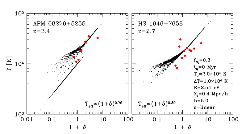
Figure 7: The temperature-density relation as derived from two sets of observed absorption-line systems (Bryan & Machacek 2000) and from the Monte-Carlo model with the same parameters set as in figure 6. The effective equation of state, $T_{\rm eff}\propto(1+\delta)^{\gamma-1}$, is calculated from the least squares linear fit between $\log(T)$ and $\log(1+\delta)$. Right panel: HS 1946+7658 at $\langle z\rangle=2.7$ (red circles), data from the Monte-Carlo model at the same redshift (black dots). Left panel: APM 08279+5255 at $\langle z\rangle=3.4$ (red circles), data from the Monte-Carlo model at the same redshift (black dots).

We run our Monte-Carlo model for a wide range of the input parameters listed in Table  2. For every set of parameters, the Monte-Carlo model provides:

1. The He III actual volume filling factor and the volume filling factor of regions with He III fraction above 0.9 as a function of redshift.

2. The mean clumping factor for all regions and for regions with He III fraction above 0.9 as a function of redshift.

3. The mean temperature as a function of redshift for the mean density regions (regions with $|\delta|<0.2$) and for all regions.

4. The He II mean optical depth as a function of redshift.

5. The IGM equation of state, i.e., the ${T-\rho}$ relation.

We compare our results with available observational data. These data include $(i)$ the mean temperature in regions of densities around the mean ($|\delta|<0.2$) estimated from nine quasars Ly$\alpha$ spectra (Schaye et al. 2000), and $(ii)$ the He II mean optical depth, $\tau_{\mbox{\scriptsize He\ {\tiny II}}}(z)$ measured from the spectrum of the quasars HS 1700+64 (Davidsen et al. 1996), Q0302-003 (Dobrzycki et al. 1991; Heap et al. 2000), and HE 2347-4342 (Smette et al. 2002; Zheng et al. 2004).

Unfortunately the available observational data are very limited. The uncertainties in the mean temperature data are large, while the uncertainties in the mean optical depth data are fairly small. There is a huge scatter in the optical depth measurements around redshift $z=2.8$ (i.e. a scatter larger than expected on the basis of the reported error bars) and it is therefore not meaningful to use these measurements to compute a mean optical depth. Nevertheless the data still provide useful constraints on the model input parameters.

As a measure of the “goodness of fit” of a given choice of parameters we use a $\chi^{2}$ statistic. For the temperature data we define $\chi^{2}_{\rm T}$ as

$$\chi^{2}_{T}=\sum\frac{(T_{\rm data}-T_{\rm model})^{2}}{\sigma_{T}^{2}}\;,$$ (19)

where the $T_{\rm data}$ are the measured temperature in the data and $T_{\rm model}$ are the model predicted temperatures at the same redshifts as the data. The estimate of the errors in the data, $\sigma_{T}$, (Schaye et al. 2000) should serve as a general guide only. We also define a $\chi^{2}$ statistic for the optical depth measurement. We interpret these data as measurements of the local optical depth rather than the mean optical depth. Therefore, we write $\chi^{2}_{\tau}$ as

$$\chi^{2}_{\tau}=\sum\frac{(\tau_{\rm data}-\tau_{\rm model})^{2}}{(\sigma_{\tau_{\rm data}}^{2}+\sigma_{\tau_{\rm model}}^{2})}\;,$$ (20)

where the $\tau_{\rm data}$ are the measured optical depth in the data and $\tau_{\rm model}$ are the model predicted mean optical depths at the same redshifts as the data. The observational errors in the data are $\sigma_{\tau_{\rm data}}$ and the scatter about the mean optical depth as estimated in the model is $\sigma_{\tau_{\rm model}}=\langle(\tau-\langle\tau\rangle)^{2}\rangle^{1/2}$ (see figure 4).

4.1 Results with a power-law $\Lambda$CDM cosmology

We first present results for the $\Lambda\rm{CDM}$ cosmological model (see Table  1). We discuss other cosmologies in section § 4.2.

In general, the best fits of the model to the observations, with $\chi_{T}^{2}\leq 1$ and $\chi_{\tau}^{2}\leq 1$, are obtained for $f_{\dot{N}_{Q}}\approx 0.3$, Jeans scale of $x_{\rm J}(z\!\!=\!\!3)\approx 0.2-0.4\ {\rm h^{-1}Mpc}$, and QSOs lifetime $t_{\rm Q}~{}\hbox to0.0pt{\raise 1.72218pt\hbox{$<$}\hss}{\lower 3.01385pt\hbox{$\sim$}}~{}10$ Myr. We found no constrains on the bias parameter $b$, and the scaling function $s$.

The initial mean temperature is $T_{0}(z\!\!=\!\!6)~{}\hbox to0.0pt{\raise 1.72218pt\hbox{$<$}\hss}{\lower 3.01385pt\hbox{$\sim$}}~{}40000$K. The temperature increment is $\Delta T\approx 10000-15000$K, which, as expected, is smaller than the estimate of Miralda-Escudé & Rees (1994) who find $\Delta T\simeq 18400$K for a fully ionized regions. This is due to energy losses by line excitation and collisional ionization in partially ionized regions. We found a correlation between the temperature increment, $\Delta T$, and the hydrogen photo-ionization heating parameter, $E$. For lower temperature increment, $\Delta T\approx 10000$K, the heating parameter is $1.27~{}\hbox to0.0pt{\raise 1.72218pt\hbox{$<$}\hss}{\lower 3.01385pt\hbox{$\sim$}}~{}E~{}\hbox to0.0pt{\raise 1.72218pt\hbox{$<$}\hss}{\lower 3.01385pt\hbox{$\sim$}}~{}3.81\ {\rm eV}$, but for higher temperature increment, $\Delta T\approx 15000$K, the heating parameter is only $E\approx 1.27\ {\rm eV}$.

Figure 3 summarizes some of our main results for the $\Lambda\rm{CDM}$ cosmology with parameters (listed in the top-left panel) for which the Monte-Carlo model yields one of the best fits to the observational data, $\chi_{T}^{2}=0.76$ and $\chi_{\tau}^{2}=0.75$.

We quantify the development of He III regions by computing the mean ionized fraction, $X$ (shown as the solid curve in panel (a) of figure 3), and the fraction of volume occupied by regions having $X>0.9$ (dashed curve). The dashed and solid curves behave as expected. The redshift at which the dashed curve reaches unity in panel (a) is $z=2.9$.

Panel (b) of figure 3 shows the evolution of the clumping factor, $f_{\rm clump}\equiv\langle 1+\sigma^{2}\rangle$, for all regions (solid curve) and for regions with $X>0.9$ (dashed curve) as a function of redshift. The clumping factor for all regions increases in time as expected. The clumping factor indicated by the dashed curve is large at high redshifts since the reionization starts in dense regions, and decreases in time until it meets the solid curve around the redshift where full reionization is established. At later times all the regions are almost completely ionized, and therefore the dashed curve follows the solid curve.

Next we examine the optical depth, $\tau_{\mbox{\scriptsize He\ {\tiny II}}}$, for helium Ly$\alpha$ absorption. This is given by

$$\tau_{i}^{\mbox{\scriptsize He\ {\tiny II}}}=\frac{c\ \sigma_{l}}{H(z)}n_{\mbox{\scriptsize He}}(1+z)^{3}(1-X_{i})(1+\delta_{i}),$$ (21)

where $H(z)$ is the Hubble constant at redshift $z$, and $\sigma_{l}={\pi e^{2}}/m_{e}c^{2}]\lambda_{l}f_{ij}\simeq 1.1\times 10^{-18}\ {\rm cm^{2}}$ is the integrated Ly$\alpha$ scattering cross section of the He II transition at wavelength $\lambda_{l}=304\ \mbox{\AA}$ and oscillator strength $f_{ij}$. At every time step, we calculate the optical depth at each point $i$, and the mean optical depth

$$\tau_{\mbox{\scriptsize He\ {\tiny II}}}=-\ln\left[\frac{1}{N}\sum_{i=1}^{N}\exp\left(-\tau_{i}^{\mbox{\scriptsize He\ {\tiny II}}}\right)\right]\;.$$ (22)

The solid line in panel (c) of figure 3 is $\tau_{\mbox{\scriptsize He\ {\tiny II}}}$ computed from our model as a function of redshift according to (22). The noise in the line is due to the limited number of points used in the Monte-Carlo model. For comparison we also show the available observational data points measured from the spectrum of the He II Gunn-Peterson effect towards the quasars HS 1700+64 (triangles, Davidsen et al. 1996), Q0302-003 (squares, Dobrzycki et al. 1991; Heap et al. 2000), and HE 2347-4342 (circles, Smette et al. 2002; Zheng et al. 2004). One can easily see a significant decrement in the optical depth from $\tau\sim 10$ at $z~{}\hbox to0.0pt{\raise 1.72218pt\hbox{$>$}\hss}{\lower 3.01385pt\hbox{$\sim$}}~{}3.5$ to $\tau~{}\hbox to0.0pt{\raise 1.72218pt\hbox{$<$}\hss}{\lower 3.01385pt\hbox{$\sim$}}~{}0.5$ at $z~{}\hbox to0.0pt{\raise 1.72218pt\hbox{$<$}\hss}{\lower 3.01385pt\hbox{$\sim$}}~{}2.5$.

In panel (a) of figure 4 we see that the rms of the fluctuations of the optical depth, $\tau_{\rm rms}=\langle(\tau-\langle\tau\rangle)^{2}\rangle^{1/2}$, behaves in a similar manner to the mean optical depth. At high redshifts, $z~{}\hbox to0.0pt{\raise 1.72218pt\hbox{$>$}\hss}{\lower 3.01385pt\hbox{$\sim$}}~{}3.5$, the high density regions get ionized while the low density regions stay neutral. This results in a large scatter of the optical depth ($\tau_{\rm rms}~{}\hbox to0.0pt{\raise 1.72218pt\hbox{$>$}\hss}{\lower 3.01385pt\hbox{$\sim$}}~{}20$). The scatter decreases towards full reionization. By $z\sim 3$, most of the high density regions are already ionized as well as a large fraction of the low density regions. At $z~{}\hbox to0.0pt{\raise 1.72218pt\hbox{$<$}\hss}{\lower 3.01385pt\hbox{$\sim$}}~{}2.5$ we have $\tau_{\rm rms}~{}\hbox to0.0pt{\raise 1.72218pt\hbox{$<$}\hss}{\lower 3.01385pt\hbox{$\sim$}}~{}1$.

Panel (d) of figure 3 shows the evolution of the mean IGM temperature as a function of redshift. The model predictions are shown as the solid and dashed curves. In each panel, the solid curve refers to the mean temperature at points with density contrast $|\delta|<0.2$, while the dashed line is the volume weighted mean temperature defined as the average temperature of all the $N$ points of the Monte-Carlo model. Overlaid as the points with error bars are the temperatures as inferred from the observations (Schaye et al. 2000). The data points correspond to temperatures in regions of mean density, and therefore they should be directly compared with the solid curves. However, the difference between the solid and dashed curves in each panel is within the error bars. The gradual variation of the model temperatures with redshift is in reasonable agreement with the data. Comparing with panel (a), we see that the temperature curves peak at the redshift for which full reionization is reached. At higher redshifts each He III particle can recombine more than once, resulting in an efficient photo-heating by the He II ionizing photons. At lower redshifts, the recombination is greatly reduced and, subsequently, the photo-heating rate decreases and adiabatic cooling dominates. At these low redshifts, the decline of the solid lines does not seem to be fast enough to match the observational data. The dashed curves, however, fall nicely among the data points. This difference between the dashed and solid curves in each panel is due to the slower adiabatic cooling of regions with $|\delta|<0.2$, relative to the overall volume weighted cooling which is dominated by the expanding low density regions.

Unsurprisingly we found a tight relation between the shape of the mean temperature curve and the combination of the heating sources $\Delta T$ and $E$. In the case we have investigated so far, with low temperature increment $\Delta T=10000$K and moderate hydrogen photo-ionization heating parameter $E=2.54\ {\rm eV}$, the temperature rises in $5000-6000$K during $3~{}\hbox to0.0pt{\raise 1.72218pt\hbox{$<$}\hss}{\lower 3.01385pt\hbox{$\sim$}}~{}z~{}\hbox to0.0pt{\raise 1.72218pt\hbox{$<$}\hss}{\lower 3.01385pt\hbox{$\sim$}}~{}4$, and never rises above 18200K. We also present two other typical cases in figure 5. In panel (a) of figure 5 we present a case of low $\Delta T=10000$K and high $E=3.81\ {\rm eV}$. In this case the rise in the temperature during reionization is around 7500K. The high hydrogen photo-ionization heating parameter does not allow the IGM to cool at higher redshifts, $4~{}\hbox to0.0pt{\raise 1.72218pt\hbox{$>$}\hss}{\lower 3.01385pt\hbox{$\sim$}}~{}z~{}\hbox to0.0pt{\raise 1.72218pt\hbox{$>$}\hss}{\lower 3.01385pt\hbox{$\sim$}}~{}6$, and the temperature reaches a maximum around 19000K. In panel (b) of figure 5 we present a case of high $\Delta T=15000$K and low $E=1.27\ {\rm eV}$. In this case the rise in the temperature during reionization exceeds 8000K and can reach 11000K. The temperature can reach a maximum of 20000K.

It is instructive to examine the temperature fluctuations in space. This can be quantified in our Monte-Carlo model by computing the rms of the temperature fluctuations, $T_{\rm rms}=\langle(T-\langle T\rangle)^{2}\rangle^{1/2}$. In panel (b) of figure 4 we show the temperature rms as a function of redshift. The temperature rms of regions with mean density (the solid lines) is affected mainly by helium photo-heating. When the IGM reaches full ionization, the photo-heating is not effective any more and the temperature rms decreases to approximately the same value as before ionization.

Finally, we consider the effect of He II ionization on the ${T-\rho}$ relation. In the absence of He II reionization, we expect a tight ${T-\rho}$ relation resulting from adiabatic cooling and photo-heating (e.g. Hui & Gnedin 1997). We assume in the Monte-Carlo model that at $z=6$ the ${T-\rho}$ relation is such that $T\propto(1+\delta)^{2/3}$. To emphasize the effect of patchy helium reionization we do not include any scatter in the ${T-\rho}$ relation at $z=6$.

Figure 6 presents the results for the same set of parameters as the above. The six panels in the figure, correspond to the ${T-\rho}$ relation at different redshifts. At the bottom of each panel, an effective equation of state of the form $T_{\rm eff}\propto(1+\delta)^{\gamma-1}$ is given. This effective equation of state is derived by the linear least square fit between $\log(T)$ and $\log(1+\delta)$.

In figure 6 we see that during the early stages of reionization, when mostly high density regions are being ionized, the slope of temperature-density relation is steepened and the scatter increases significantly. At $z\sim 3-4$ a non-negligible scatter of about $50\%$ is introduced. Around $z=3$, where the reionization of low density regions is much more significant, the slope of temperature-density relation flattens. When the helium in the IGM is fully ionized the photo-ionization heating becomes inefficient and the main process affecting the gas temperature is adiabatic cooling. The cooling reduces the scatter, and by $z=1$ a tight ${T-\rho}$ relation is restored.

In figure 7 we present the ${T-\rho}$ relation as derived from two sets of observed quasar absorption-line systems from Bryan & Machacek (2000): APM 08279+5255 at $\langle z\rangle=3.4$ (left panel) and HS 1946+7658 at $\langle z\rangle=2.7$ (right panel), and compare with the ${T-\rho}$ relation from the Monte-Carlo model at the same redshifts.

At $z=2.7$ the slope of the effective equation of state from the model, $\gamma_{\rm model}=1.392\pm 0.002$, fits the slope of the data from the HS 1946+7658 absorption-lines, $\gamma_{\rm data}=1.31\pm 0.15$, within $0.6\sigma$. At $z=3.4$ the slope of the effective equation of state from the model, $\gamma_{\rm model}=1.748\pm 0.008$, fits the slope of the data from the APM 08279+5255 absorption-lines, $\gamma_{\rm data}=1.55\pm 0.14$, within $1.4\sigma$. The coefficient of the effective equation of state from the model fits the data from the observations within $1.2\sigma$ at $z=2.7$ and within $0.3\sigma$ at $z=3.4$.

Figure 8: The slope, $\gamma$, of the effective equation of state, $T_{\rm eff}\propto(1+\delta)^{\gamma-1}$, at the mean density. The open circles are the slopes calculated from the nine QSO Ly$\alpha$ spectra in panel (d) of figure 3 by Schaye et al. 2000. The filled circles are the slopes calculated from the Monte-Carlo model for regions with $|\delta|<0.2$ at the same redshifts. $1\sigma$ error bars in $\gamma$ are presented for both the observational data and the model points.

In figure 8 we present the slopes, $\gamma$, of the effective equation of state at the mean density of the nine quasar Ly$\alpha$ spectra studied by from Schaye et al. (2000; open circles) and the slopes calculated from the Monte-Carlo model from regions with $|\delta|<0.2$ at the same redshifts (filled circles). As expected, the reheating of the gas at the time of reionization, $z\sim 3-4$, causes a decrease in $\gamma$. After the reionization the IGM gradually evolves again towards an ionization equilibrium and $\gamma$ increases. To compare between the slopes from the observational data and the slopes from the model we calculated $\eta$, the distance in $\sigma$ between the two $\gamma$,

$$\eta=\frac{|\gamma_{\rm data}-\gamma_{\rm model}|}{\sqrt{\sigma^{2}_{\rm data}+\sigma^{2}_{\rm model}}}\;,$$ (23)

where $\gamma_{\rm data}$ and $\sigma_{\rm data}$ are the observational data slopes and their $1\sigma$ errors, and $\gamma_{\rm model}$ and $\sigma_{\rm model}$ are the Monte-Carlo model slopes and their $1\sigma$ errors (see Table 3). From figure 8 one can see that in general $\gamma$ from the Monte-Carlo model have higher values then $\gamma$ from the observational data, although for most redshifts $\eta<3$ (see Table 3).

Table 3: Comparison between the slopes, $\gamma$, of the effective equation of state at the mean density from the observations (Schaye et al. 2000) and the slopes from the Monte-Carlo model (from regions with $|\delta|<0.2$). $z$ is the redshift with the errors from the observational data. $\gamma_{\rm data}$ is the slope from the observational data. $\gamma_{\rm model}$ is the slope from the Monte-Carlo model. $\eta$ is the distance in $\sigma$ between the model slope and the observational data slope.

$z$	$\gamma_{\rm data}$	$\gamma_{\rm model}$	$\eta$
$4.307_{-0.161}^{+0.121}$	$1.315_{-0.491}^{+0.268}$	$1.68\pm 0.03$	$1.35$
$3.911_{-0.098}^{+0.095}$	$1.094_{-0.415}^{+0.680}$	$1.75\pm 0.04$	$0.96$
$3.836_{-0.148}^{+0.179}$	$1.443_{-0.432}^{+0.541}$	$1.78\pm 0.04$	$0.62$
$3.721_{-0.112}^{+0.090}$	$1.293_{-0.290}^{+0.114}$	$1.81\pm 0.05$	$4.16$
$3.551_{-0.122}^{+0.146}$	$1.505_{-0.227}^{+0.383}$	$1.96\pm 0.06$	$1.17$
$3.365_{-0.142}^{+0.164}$	$1.110_{-0.123}^{+0.081}$	$1.83\pm 0.06$	$7.13$
$3.234_{-0.084}^{+0.185}$	$0.589_{-0.435}^{+0.685}$	$1.58\pm 0.04$	$1.44$
$3.076_{-0.171}^{+0.145}$	$1.045_{-0.100}^{+0.076}$	$1.39\pm 0.01$	$4.50$
$3.001_{-0.109}^{+0.138}$	$0.958_{-0.142}^{+0.139}$	$1.38\pm 0.01$	$3.02$
$2.841_{-0.129}^{+0.104}$	$1.215_{-0.281}^{+0.145}$	$1.411\pm 0.004$	$1.35$
$2.658_{-0.109}^{+0.221}$	$0.899_{-0.069}^{+0.315}$	$1.448\pm 0.004$	$1.74$
$2.593_{-0.109}^{+0.116}$	$1.203_{-0.034}^{+0.093}$	$1.460\pm 0.003$	$2.75$
$2.495_{-0.161}^{+0.130}$	$1.563_{-0.110}^{+0.094}$	$1.476\pm 0.003$	$0.85$
$2.285_{-0.058}^{+0.094}$	$1.274_{-0.176}^{+0.301}$	$1.503\pm 0.002$	$0.76$
$2.211_{-0.114}^{+0.117}$	$1.310_{-0.319}^{+0.216}$	$1.510\pm 0.002$	$0.93$
$1.961_{-0.113}^{+0.127}$	$1.389_{-0.417}^{+0.228}$	$1.534\pm 0.002$	$0.64$

4.2 Results with the RSI and OCDM cosmologies

We have also run our Monte-Carlo model for the RSI and the OCDM cosmological models (see Table 1) and have tried to fit the model parameters to the observations of the mean optical depth and mean temperature. We found no major differences among the results in the three cosmological models we consider

As in the $\Lambda\rm{CDM}$ cosmology, by fitting the observations with $\chi_{T}^{2}\leq 1$ and $\chi_{\tau}^{2}\leq 1$, we get $f_{\dot{N}_{Q}}\approx 0.3$ for both the RSI and the OCDM models. The QSOs lifetime in the RSI and the OCDM models is $t_{\rm Q}~{}\hbox to0.0pt{\raise 1.72218pt\hbox{$<$}\hss}{\lower 3.01385pt\hbox{$\sim$}}~{}5$ Myr. A Jeans scale length of $x_{\rm J}(z\!\!=\!\!3)\approx 0.1-0.4\ {\rm h^{-1}Mpc}$ fits the RSI model, while $x_{\rm J}(z\!\!=\!\!3)\approx 0.2-0.4\ {\rm h^{-1}Mpc}$ fits the $\Lambda\rm{CDM}$, and only $x_{\rm J}(z\!\!=\!\!3)\approx 0.4\ {\rm h^{-1}Mpc}$ fits the OCDM model. While in $\Lambda\rm{CDM}$ the bias parameter is not constrained, we find $b\approx 2-8$ and $b\approx 2-3$ for the RSI and OCDM models, respectively. As in the $\Lambda\rm{CDM}$ cosmology, we found no constrains on the scaling function (equation 6c). In the RSI and OCDM cosmological models the initial mean temperature is $T_{0}(z\!\!=\!\!6)~{}\hbox to0.0pt{\raise 1.72218pt\hbox{$<$}\hss}{\lower 3.01385pt\hbox{$\sim$}}~{}30000$K, and temperature increment of $\Delta T\approx 10000-15000$K. For $\Delta T\approx 10000$K the hydrogen photo-ionization heating parameter varies between $2.54~{}\hbox to0.0pt{\raise 1.72218pt\hbox{$<$}\hss}{\lower 3.01385pt\hbox{$\sim$}}~{}E~{}\hbox to0.0pt{\raise 1.72218pt\hbox{$<$}\hss}{\lower 3.01385pt\hbox{$\sim$}}~{}3.81\ {\rm eV}$ while in the $\Lambda\rm{CDM}$ model $1.27~{}\hbox to0.0pt{\raise 1.72218pt\hbox{$<$}\hss}{\lower 3.01385pt\hbox{$\sim$}}~{}E~{}\hbox to0.0pt{\raise 1.72218pt\hbox{$<$}\hss}{\lower 3.01385pt\hbox{$\sim$}}~{}3.81\ {\rm eV}$. In all cosmological models, the heating parameter is $1.27\ {\rm eV}$ for $\Delta T\approx 15000$K .

5 Discussion

Figure 9: The filling factor, temperature and optical depth evolution as a function of redshift in a $\Lambda\rm{CDM}$ cosmology for $f_{\dot{N}_{Q}}=1.0$ (right panels) $f_{\dot{N}_{Q}}=0.2$ (left panels). For $f_{\dot{N}_{Q}}=1.0$ the set of parameters gives $\chi_{T}^{2}=2.3$ and $\chi_{\tau}^{2}=7.9$, and for $f_{\dot{N}_{Q}}=0.2$, $\chi_{T}^{2}=3.2$ and $\chi_{\tau}^{2}=0.1$.

Table 4: Summary of the best fit parameters derived from comparison with the observed optical depth and temperature evolution for $\chi_{T}^{2}\leq 1$ and $\chi_{\tau}^{2}\leq 1$. “N.C.” implies no constraints on the parameter in the relevant range.

	$\Lambda\rm{CDM}$	RSI	OCDM
$f_{\dot{N}_{\rm Q}}$	$0.3$	$0.3$	$0.3$
$t_{\rm Q}$	$~{}\hbox to0.0pt{\raise 1.72218pt\hbox{$<$}\hss}{\lower 3.01385pt\hbox{$\sim$}}~{}10$	$~{}\hbox to0.0pt{\raise 1.72218pt\hbox{$<$}\hss}{\lower 3.01385pt\hbox{$\sim$}}~{}5$	$~{}\hbox to0.0pt{\raise 1.72218pt\hbox{$<$}\hss}{\lower 3.01385pt\hbox{$\sim$}}~{}5$	Myr
$T_{0}(z\!\!=\!\!6)$	$~{}\hbox to0.0pt{\raise 1.72218pt\hbox{$<$}\hss}{\lower 3.01385pt\hbox{$\sim$}}~{}4.0$	$~{}\hbox to0.0pt{\raise 1.72218pt\hbox{$<$}\hss}{\lower 3.01385pt\hbox{$\sim$}}~{}3.0$	$~{}\hbox to0.0pt{\raise 1.72218pt\hbox{$<$}\hss}{\lower 3.01385pt\hbox{$\sim$}}~{}3.0$	$10^{4}$K
$\Delta T$	$1.0-1.5$	$1.0-1.5$	$1.0-1.5$	$10^{4}$K
$E$	$1.27-3.81$	$1.27-3.81$	$1.27-3.81$	$\ {\rm eV}$
$x_{\rm J}(z\!\!=\!\!3)$	$0.2-0.4$	$0.1-0.4$	$0.4$	$\ {\rm h^{-1}Mpc}$
$b$	N.C.	$2-8$	$2-3$
$s$	N.C.	N.C.	N.C.
$z_{\rm ion}$	$2.8-2.9$	$2.8-2.9$	$2.8-2.9$

We have presented a model for following the thermal properties of the IGM during patchy He II reionization. The model assumes that radiation from QSOs is the main cause of He II reionization and neglects the contribution from galaxies. This is consistent with our finding that the model can account for He II reionization in a way consistent with the available observations of the mean temperature and He II optical depth. Further, according to the galform semi-analytic model for galaxy formation the contribution of galaxies to the He II ionizing radiation is negligible compared to QSOs even at redshifts as high as $z\sim 6$. We have also neglected contributions from thermal emission in shock heated gas (Miniati et al. 2004) and also from redshifted soft X-ray produced at $z\sim 20$ (Ricotti & Ostriker 2004). These contributions could be important for He II, especially at $z>3$, and will be studied in detail in a future paper.

We have considered three different cosmological models: standard power-law $\Lambda\rm{CDM}$, $\Lambda\rm{CDM}$ with a running spectral index (RSI), and an open CDM and found no significant differences between them. Table 4 lists the input parameters for which the Monte-Carlo model matches best the observational data.

A key parameter is the emission factor $f_{\dot{N}_{Q}}$ which multiplies the overall emission rate derived from the MHR luminosity function. In all cosmologies, an emission factor of $f_{\dot{N}_{Q}}=1$ yields results that are inconsistent with the relevant observational data (see panels on the right of figure 9). For $f_{\dot{N}_{Q}}=1$, reionization occurs too early at $z=4.1$, and shifts the typical behaviour of the mean temperature and optical depth to earlier times. Too low a value for $f_{\dot{N}_{Q}}$ does not match the data either. For $f_{\dot{N}_{Q}}=0.2$ the reionization occurs too late ($z\approx 2.5$), and the mean optical depth does not reach high enough values around $z=3$ (see panels on the left of figure 9). To match the data we need $f_{\dot{N}_{Q}}\approx 0.3$. This result agrees with several observations (Giroux & Shull 1997; Savaglio et al. 1997; Songaila 1998; Kepner et al. 1999; Smette et al. 2002) and simulations (Theuns et al. 1998; Efstathiou et al. 2000) which suggest a softer UV radiation field than the standard UV background due to QSOs emission.

The He III fraction rises modestly at the initial stages of reionization. The rise becomes more rapid as the He III fraction gets close to unity (full reionization), at redshift $z_{\rm ion}$. In the simulations of Sokasian et al. (2002) the full reionization occurs at a redshift of $z\approx 3.8$ (see their figure 3, models 1-3), while we found that full reionization is never achieved before $z_{\rm ion}=3$. The reason for this difference is that we tune our model to match the temperature evolution. In our model the temperature increases until full reionization is reached, and declines monotonically afterwards.

The optical depth, for He II Ly$\alpha$ absorption, is $\tau_{\mbox{\scriptsize He\ {\tiny II}}}\sim 10$ at $z~{}\hbox to0.0pt{\raise 1.72218pt\hbox{$>$}\hss}{\lower 3.01385pt\hbox{$\sim$}}~{}3.5$ with a slow decline. Around $z_{\rm ion}$ the decline is much more rapid, from $\tau_{\mbox{\scriptsize He\ {\tiny II}}}\sim 10$ at $z\sim 3.5$, to $\tau_{\mbox{\scriptsize He\ {\tiny II}}}\sim 0.5$ at $z\sim 2.5$. At $z~{}\hbox to0.0pt{\raise 1.72218pt\hbox{$<$}\hss}{\lower 3.01385pt\hbox{$\sim$}}~{}2.5$ the decline is gradual again and reached $\tau_{\mbox{\scriptsize He\ {\tiny II}}}\sim 0.3$ at $z=1.0$. We need more observational data to have better constrains on Monte-Carlo model parameters. Sokasian et al. (2002) also compute the mean optical depth in their simulations, however, they show results up to $z=2.8$. Some of their models also match the observations up to that redshift, but we cannot make a more direct comparison of their models with ours at lower redshifts.

An important application of the model is to study the temperature-density relation in the IGM. Patchy He II reionization is expected to produce a $50\%$ scatter in this relation at $3<z<4$ (see also Hui & Haiman 2003). At lower redshifts, when the helium in the IGM becomes fully ionized, photo-heating is not effective anymore and the main process governing the gas temperature is adiabatic cooling. The scatter is then reduced and a tight $T-\rho$ is rapidly established. The increase in the scatter at $3<z<4$ should be taken into account in the analysis of the Ly$\alpha$ forest data and can be detected in high resolution spectra. The temperature-density relation from our Monte-Carlo model fits the data from Bryan & Machacek (2000) around $z\sim 3$ reasonably well, but more observational data is needed, especially in low density regions, to be able to put better constrains on the model.

The model predicts a gradual rise in the mean temperature between $z\sim 4$ and $z\sim 3$. Our results match the observed mean temperature as a function of redshift (Schaye et al. 2000). A possible discrepancy is that adiabatic cooling is not efficient enough to cause a rapid decline in the temperature at $z~{}\hbox to0.0pt{\raise 1.72218pt\hbox{$<$}\hss}{\lower 3.01385pt\hbox{$\sim$}}~{}2$, as the observations indicate. However, the observational situation is still inconclusive. Although the temperature increase inferred from the observations is probably robust (Theuns et al. 2002), the quantitative behaviour is less certain.

There is a weak degeneracy between the temperature increment, $\Delta T$, and the energy, $E$, corresponding to photo-heating by the diffuse hydrogen ionizing background. An energy of $E\sim 1.27\ {\rm eV}$ works well with the full range $10000~{}\hbox to0.0pt{\raise 1.72218pt\hbox{$<$}\hss}{\lower 3.01385pt\hbox{$\sim$}}~{}\Delta T~{}\hbox to0.0pt{\raise 1.72218pt\hbox{$<$}\hss}{\lower 3.01385pt\hbox{$\sim$}}~{}15000$K. On the other hand the higher energies $E\sim 2.54-3.81\ {\rm eV}$ works only with $\Delta T$ close to $10000$K. In any case, the inferred values for $\Delta T$ are consistent with the assumption that due to energy loses in partially ionized regions the temperature increment must be smaller then the estimates of Miralda-Escudé & Rees (1994) for fully ionized regions.

We have also found that only short QSO lifetimes fit the data: $t_{\rm Q}~{}\hbox to0.0pt{\raise 1.72218pt\hbox{$<$}\hss}{\lower 3.01385pt\hbox{$\sim$}}~{}10$ Myr for the $\Lambda\rm{CDM}$ model and $t_{\rm Q}~{}\hbox to0.0pt{\raise 1.72218pt\hbox{$<$}\hss}{\lower 3.01385pt\hbox{$\sim$}}~{}5$ Myr for the RSI and OCDM models. The initial mean temperature has an upper limit of $T_{0}(z\!\!=\!\!6)\approx 40000$K for the $\Lambda\rm{CDM}$ model and an upper limit of $T_{0}(z\!\!=\!\!6)\approx 30000$K for the RSI and OCDM models. The Jeans scale length of $x_{\rm J}(z\!\!=\!\!3)\approx 0.1-0.4\ {\rm h^{-1}Mpc}$ fits the RSI model, while $x_{\rm J}(z\!\!=\!\!3)\approx 0.2-0.4\ {\rm h^{-1}Mpc}$ fits the $\Lambda\rm{CDM}$, and only $x_{\rm J}(z\!\!=\!\!3)\approx 0.4\ {\rm h^{-1}Mpc}$ fits the OCDM model. While in $\Lambda\rm{CDM}$ the bias parameter is not constrained, in RSI $b\approx 2-8$ and in OCDM $b\approx 2-3$. In all cosmologies we found no constrains on the scaling function.

In numerical hydrodynamical simulations of the Ly$\alpha$ forest He II reionization is often modelled as a result of a uniform ionizing background of photons. This recipe for He II reionization leads to a sudden jump in the mean IGM temperature at about $z\sim 3$. Our findings imply that this recipe is oversimplified and may lead to incorrect conclusions. An incorporation of models similar to ours in this type of simulation is needed.

The distribution of the column densities ratio $\eta=N(\mbox{He\ {\footnotesize II}})/N(\mbox{H\ {\footnotesize I}})$ contains important information on the properties of the ionizing sources (e.g. FUSE observations, Zheng et al. 2004). Therefore, it will be very interesting to look at the distribution of $\eta$ as a diagnostic of the reionization epoch. To do so one must include H I reionization, and therefore to take into account the ionizing radiation from galaxies. It is not trivial to add it to our Monte-Carlo model since the model is based on the assumption that the ionizing sources are short lived, which is incorrect for galaxies. Therefore, adding the ionizing radiation from galaxies requires a different approach which will be presented in a future paper.

Appendix A The QSO ionizing photon emission rate

Our calculation of the QSO emission rate of He II ionizing photons per unit comoving volume is based on MHR for hydrogen. First we calculate the QSO emission rate in a flat universe without a cosmological constant ($\Omega_{0}=1$, $\Omega_{\Lambda}=0$). Later in Appendix A.6 we extend this calculation to fit all cosmologies with any desirable $\Omega_{0}$ and $\Omega_{\Lambda}$.

A.1 QSO luminosity function

Following MHR we represent the quasar blue luminosity function ($\lambda_{\rm B}=4400\ \mbox{\AA}$) as a double power-law:

$$\phi(L,z)=\frac{\phi_{\ast}/L_{\ast}(z)}{[L_{B}/L_{\ast}(z)]^{\beta_{1}}+[L_{B}/L_{\ast}(z)]^{\beta_{2}}},$$ (24)

where $\beta_{1}$ and $\beta_{2}$ are the power-law indices for faint and bright quasars, respectively. The position of the break $L_{\ast}(z)$ is

$$L_{\ast}(z)=L_{\ast}(0)(1+z)^{\alpha_{s}-1}\frac{e^{\zeta z}(1+e^{\xi z_{\ast}})}{e^{\xi z}+e^{\xi z_{\ast}}},$$ (25)

where

$$L_{\ast}(0)=L_{\odot}\!\times\!10^{-0.4[M_{\ast}(0)-M_{\odot}]}=4.67\!\times\!10^{29}\ {\rm erg\ Hz^{-1}s^{-1}},$$ (26)

$M_{\odot}=5.48$ and $L_{\odot}=3.44\times 10^{18}\ {\rm erg\ Hz^{-1}s^{-1}}$ are the Solar magnitude and luminosity respectively, and the rest of the luminosity parameters can be found in Table 5.

In Table 5 $\phi_{\ast}$ is given for a Hubble constant $h=0.5$. From this value we calculate $\phi_{\ast}(h)$ as a function of $h$:

$$\phi_{\ast}(h)=8.9125\times\left(\frac{h}{0.5}\right)^{3}\times 10^{-7}\ {\rm Mpc^{-3}}.$$ (27)

Table 5: Parameters of the double power-law luminosity function (Pei 1995; MHR).

Parameter	Value
$\beta 1$ …………………………	$1.64$
$\beta 2$ …………………………	$3.52$
$z_{\ast}$ …………………………	$1.9$
$\zeta$ …………………………..	$2.58$
$\xi$ …………………………..	$3.16$
$M_{\ast}(0)$ ……………………	$-22.35$
$\log[\phi_{\ast}(h_{50})/{\rm Gpc^{-3}}]$ …	$2.95$

A.2 The QSO spectral energy distribution

The luminosity spectrum of a “typical” QSO is assumed to have a power-law spectral energy distribution (SED), $L(\nu)\propto\nu^{-\alpha_{s}}$, with different slopes in different wavelength ranges (MHR),

$$L(\nu)\propto\left\{\begin{array}[]{ll}\nu^{-0.3}&(2500\ \mbox{\AA}<\lambda<4400\ \mbox{\AA})\\ \nu^{-0.8}&(1050\ \mbox{\AA}<\lambda<2500\ \mbox{\AA})\\ \nu^{-1.8}&(\lambda<1050\ \mbox{\AA})\end{array}\right..$$ (28)

The QSO ionizing flux, $S$, is the number of ionizing photons emitted by a QSO per second,

$$S=\int_{\nu_{i}}^{\nu_{f}}L(\nu)\frac{{\rm d}\nu}{h\nu},$$ (29)

where $h$ is the Planck constant. For convenience we represent $S$ as a function of wavelength, $\lambda$, and since the ionization wavelength of helium ($\lambda=228\ \mbox{\AA}$) is less then $1050\ \mbox{\AA}$,

$$S=\frac{L_{B}}{1.8h}\left(\frac{4400}{2500}\right)^{-0.3}\left(\frac{2500}{1050}\right)^{-0.8}\left(\frac{1050}{\lambda}\right)^{-1.8}\left|\begin{array}[]{l}{}^{228\ \mbox{\AA}}\\ {}_{0\ \mbox{\AA}}\end{array}\right.,$$ (30)

where $L_{B}$ is the luminosity in the blue band (in units of $\ {\rm erg\ Hz^{-1}s^{-1}}$), and neglecting ionization of heavier elements.

A.3 QSO ionizing flux function

Equations (24) and (30) allow us to write the number of emitted ionizing photons per unit time per unit (comoving) volume as

$$\Phi(S,z)=\frac{\phi_{\ast}/S_{\ast}(z)}{[S/S_{\ast}(z)]^{\beta_{1}}+[S/S_{\ast}(z)]^{\beta_{2}}},$$ (31)

where $S_{\ast}(z)$ for helium ionization is

$$S_{\ast}(z)=\frac{L_{\ast}(z)}{1.8h}\left(\frac{4400}{2500}\right)^{-0.3}\left(\frac{2500}{1050}\right)^{-0.8}\left(\frac{1050}{\lambda}\right)^{-1.8}\left|\begin{array}[]{l}{}^{228\ \mbox{\AA}}\\ {}_{0\ \mbox{\AA}}\end{array}\right.$$

$$\ \ \ \ \ \ \ \ \ \!\!=1.057\!\times\!10^{54}(1+z)^{\alpha_{s}-1}\frac{e^{\zeta z}(1+e^{\xi z_{\ast}})}{e^{\xi z}+e^{\xi z_{\ast}}}\ {\rm phot\ s^{-1}}.$$ (32)

A.4 K-Correction

Taking into account the wavelength dependence of the power $\alpha_{s}$ in the QSO spectrum, one should replace the K-correction $(1+z)^{\alpha_{s}-1}$ in equation (32), with

$$K_{c}(z)=\left\{\begin{array}[]{ll}(1+z)^{0.3-1}&(2500\ \mbox{\AA}<\frac{4400\ \mbox{\AA}}{1+z}<4400\ \mbox{\AA})\\ K_{1}(1+z)^{0.8-1}&(1050\ \mbox{\AA}<\frac{4400\ \mbox{\AA}}{1+z}<2500\ \mbox{\AA})\\ K_{1}K_{2}(1+z)^{1.8-1}&(\frac{4400\ \mbox{\AA}}{1+z}<1050\ \mbox{\AA})\end{array}\right.,$$ (33)

where $K_{1}=\left(\frac{4400}{2500}\right)^{0.3-0.8}$ and $K_{2}=\left(\frac{4400}{1050}\right)^{0.8-1.8}$.

A.5 The QSOs emission rate of ionizing photons per unit comoving volume

The QSO emission rate of ionizing photons per unit comoving volume can be written as

$$\dot{N}_{\rm Q}(z)=\int_{S_{min}}^{\infty}\Phi(S,z)S{\rm d}S.$$ (34)

where $S_{min}=0.018S_{\ast}(0)$ corresponds to $M_{B}\approx-18$, and therefore $L_{min}\approx 0.018L_{\ast}(0)$ (Cheng et al. 1985). Using equation (31) we write $\dot{N}_{\rm Q}(z)$ as

$$\dot{N}_{\rm Q}(z)=\phi_{\ast}(h)S_{\ast}(z)\int_{0.018}^{\infty}\frac{x{\rm d}x}{x^{\beta_{1}}+x^{\beta_{2}}},$$ (35)

where $x\equiv S/S_{\ast}(z)$. Numerical integration gives

$$\int_{0.018}^{\infty}\frac{x{\rm d}x}{x^{\beta_{1}}+x^{\beta_{2}}}=2.298.$$ (36)

Equations (35), (27) and (32) yield the QSO emission rate of helium-ionizing photons

$$\dot{N}_{\rm Q}(z)=2.16\!\times\!10^{48}K_{c}(z)\frac{e^{\zeta z}(1+e^{\xi z_{\ast}})}{e^{\xi z}+e^{\xi z_{\ast}}}\left(\frac{h}{0.5}\right)^{3}\ {\rm s^{-1}Mpc^{-3}}.$$ (37)

A.6 The cosmological factor

Untill now we assumed a flat universe cosmology with $\Omega_{0}=1$ and $\Omega_{\Lambda}=0$. To obtain $\dot{N}_{\rm Q}(z)$ in different cosmologies we multiply the above result by a cosmological factor $f_{cosmo}(\Omega_{0},\Omega_{\Lambda})$ so that

$$\dot{N}_{\rm Q}(z)\Longrightarrow f_{cosmo}(\Omega_{0},\Omega_{\Lambda})\dot{N}_{\rm Q}(z),$$ (38)

where

$$f_{cosmo}(\Omega_{0},\Omega_{\Lambda})=\frac{{\rm d}r_{\rm c}(1,0)/{\rm d}z}{{\rm d}r_{\rm c}(\Omega_{0},\Omega_{\Lambda})/{\rm d}z}$$

$$\ \ \ \ \ \ \ \ \ \ \ \ \ \ \ \ \ \ \ \ =\sqrt{(1-a)\Omega_{0}+(a^{3}-a)\Omega_{\Lambda}+a},$$ (39)

and ${\rm d}r_{\rm c}/{\rm d}z$ is the rate of change of comoving distance with redshift.

Appendix B The number of absorbed photons per redshift interval bin

We write the total number of ionizing photons that were absorbed at time interval $[t,t+\Delta t]$ as

$$N_{\rm abs}(z)=\left[\dot{N}_{\rm Q}(z)\Delta t+N_{\rm trs}\right]\left[1-e^{-c\Delta t/l_{\rm ph}(z)}\right],$$ (40)

where $\dot{N}_{\rm Q}(z)$ is the QSO ionizing photon emission rate per unit comoving volume, $\Delta t$ is the time step, $N_{\rm trs}$ is the number of photons received from previous time intervals, and the mean free path of the He II ionizing photons is

$$l_{\rm ph}(z)=\left[n_{\mbox{\scriptsize He\ {\tiny II}}}(1+\delta(z))(1+z)^{3}\sigma_{\rm ion}\right]^{-1},$$ (41)

where $n_{\mbox{\scriptsize He\ {\tiny II}}}$ is the mean comoving number density of He II, $\delta(z)$ is the local density perturbation, and $\sigma_{\rm ion}$ is the mean ion-photon cross section for He II.

The ion-photon cross section at frequency $\nu$ is

$$\sigma_{\rm ion}(\nu)=8.61\times 10^{-18}\ {\rm cm^{2}}\left(\frac{\nu}{\nu_{\mbox{\scriptsize He\ {\tiny II}}}}\right)^{-4}\frac{e^{-4\arctan\epsilon/\epsilon}}{1-e^{-2\pi/\epsilon}},$$ (42)

where $\epsilon=[\nu/\nu_{\mbox{\scriptsize He\ {\tiny II}}}-1]^{-1/2}$, and $\nu_{\mbox{\scriptsize He\ {\tiny II}}}=1.3\times^{16}{\rm Hz}$ is the frequency at the He II ionization energy, $E=54.42\ {\rm eV}$ (Cen 1992).

Following Theuns et al. (1998) we approximate the Cen (1992) ion-photon cross section as having simple power-low dependence on frequency

$$\sigma_{\rm ion}(\nu)=1.9\times 10^{-18}\ {\rm cm^{2}}\left(\frac{\nu}{\nu_{\mbox{\scriptsize He\ {\tiny II}}}}\right)^{-3}.$$ (43)

B.1 Frequency binning

Because of the frequency dependency of the cross section we divide the frequency interval of ionizing photons into 10 bins, from $\nu_{\mbox{\scriptsize He\ {\tiny II}}}$ to infinity, and calculate the total number of absorbed photons in each bin. We define the luminosity as the photons energy rate per frequency (in units of $\ {\rm erg\ Hz^{-1}s^{-1}}$). The luminosity of a “typical” QSO at wavelengths $\lambda<1050\ \mbox{\AA}$ is assumed to behave as $L(\nu)\propto\nu^{-1.8}$ (equation 28). To have equal luminosity in each bin, we choose the frequency at the edge of every bin $j$ to be

$$\nu^{j+1}=\nu_{1050}\left[\left(\frac{\nu^{j}}{\nu_{1050}}\right)^{-1.8}-f_{\rm B}\left(\frac{\nu_{\mbox{\scriptsize He\ {\tiny II}}}}{\nu_{1050}}\right)^{-1.8}\right]^{-1/1.8},$$ (44)

where $\nu_{1050}=2.85\times 10^{15}{\rm Hz}$ is the frequency at wavelength $\lambda=1050\ \mbox{\AA}$, and $f_{\rm B}=0.1$ is 1 over the number of bins. For each bin we calculated the mean ion-photon cross section

$$\sigma_{\rm ion}^{j} = \sigma_{0}^{\rm ion}\frac{\int_{\nu^{j}}^{\nu^{j+1}}\left(\frac{\nu}{\nu_{\mbox{\scriptsize He\ {\tiny II}}}}\right)^{-3}\left(\frac{\nu}{\nu_{1050}}\right)^{-1.8}{\rm d}\nu}{\int_{\nu^{j}}^{\nu^{j+1}}\left(\frac{\nu}{\nu_{1050}}\right)^{-1.8}{\rm d}\nu}$$ (45)

$$= \sigma_{0}^{\rm ion}(\nu_{\mbox{\scriptsize He\ {\tiny II}}})^{3}\frac{\int_{\nu^{j}}^{\nu^{j+1}}\nu^{-4.8}{\rm d}\nu}{\int_{\nu^{j}}^{\nu^{j+1}}\nu^{-1.8}{\rm d}\nu},$$

and the QSO ionizing photon emission rate

$$\dot{N}_{\rm Q}^{j}(z)=f_{\rm B}\dot{N}_{\rm Q}(z).$$ (46)

B.2 The number of absorbed photons

To get more accurate results for the radiative transfer we first calculate the number of redshifted photons that were transferred to a lower frequency bin. Next, since we choose 10 frequency bin we solve a set of 10 differential equations for the photon transmission,

$$\frac{{\rm d}N_{\rm trs}^{i}}{{\rm d}t}\!=\!\left(\!N_{0}(z)\!-\!n_{\rm He\ II}\!-\!\sum_{j=1}^{10}\!N_{\rm trs}^{j}(z)\!\right)\!c\sigma_{\rm ion}^{i}N_{\rm trs}^{i}(z),$$ (47)

where $N_{0}(z)=\sum_{j=1}^{10}\dot{N}_{\rm Q}^{j}(z)\Delta t\!+\!N_{\rm trs}^{j}(z)$ is the total number of photons that are available for ionization and $N_{\rm trs}^{j}$ is the previous number of transmitted photons in bin $j$. The actual number of the absorbed ionizing photons is

$$N_{\rm abs}(z)=N_{0}(z)-\sum_{j=1}^{10}N_{\rm trs}^{j}(z).$$ (48)

Appendix C The gas density field

We assume that the gas density traces the dark matter density smoothed over the Jeans length scale, $x_{\rm J}$, determined by the balance of pressure and gravitational forces. Under this assumption we compute the variance of the gas density field, $\sigma^{2}$, from the dark matter nonlinear (dimensionless) power spectrum, $\Delta^{2}_{NL}(k)$ and a smoothing window function, $f_{k}$,

$$\sigma^{2}=\int\Delta^{2}_{NL}(k)|f_{k}|^{2}\frac{{\rm d}k}{k}\;.$$ (49)

We use the recipe outlined in Peacock (1999) to derive the nonlinear power spectrum from the linear one. For the smoothing window we choose a Gaussian function $f_{k}=e^{-k^{2}x_{\rm J}^{2}/2}$ (Hui & Gnedin 1997, Nusser 2000), where $x_{\rm J}$ is the Jeans length scale.

The clumping factor can be defined as

$$f_{\rm clump}=\frac{\langle\rho^{2}\rangle}{\langle\rho\rangle^{2}}=\langle(1+\delta)^{2}\rangle=1+\langle\delta^{2}\rangle,$$ (50)

where $\rho=\langle\rho\rangle(1+\delta)$ is the gas density at any point in the universe, $\langle\rho\rangle$ is the mean gas density, and $\delta$ is the density fluctuation.

References

- [1] Adelberger K. L., Steidel C. C., Shapley A. E., Pettini M., 2003, ApJ, 584, 45
- [2] Aracil B., Petitjean P., Pichon C., Bergeron J., 2004, A&A, 419, 811
- [3] Baugh C. M., Lacey C. G., Frenk C. S., Granato G. L., Silva L., Bressan A., Benson A. J., Cole S., 2004, submitted to MNRAS (astro-ph/0406069)
- [4] Becker R. H., Fan, X., White, R. L., Strauss, M. A., Narayanan, V. K., Lupton R. H., Gunn, J. E. Annis J., Bahcall N. A., Brinkmann J., Connolly A. J., Csabai I., Czarapata P. C., Doi M., Heckman T. M., Hennessy, G. S., Ivezic Z., Knapp G. R., Lamb D. Q., McKay T. A., Munn J. A., Nash T., Nichol, R., Pier J. R., Richards G. T., Schneider D. P., Stoughton C., Szalay A. S., Thakar A. R., York, D. G., 2001, AJ, 122, 2850
- [5] Benson A. J., Nusser A., Sugiyama N., Lacey C. G., 2001, MNRAS, 320, 153
- [6] Benson A. J., Lacey C. G., Baugh C. M., Cole S., Frenk, C. S., 2002, MNRAS, 333, 156
- [7] Bryan G. L., Machacek M. E., 2000, ApJ, 534, 57
- [8] Bi H., Davidsen A.F., 1997, ApJ, 479, 523
- [9] Cen, R., 1992, ApJ, 78, 341
- [10] Cen, R., 2003, ApJ, 591, 12
- [11] Cheng F. Z., Danese L., De Zotti G., Franceschini A., 1985, MNRAS, 212, 857
- [12] Cole S., Lacey C. G., Baugh C. M., Frenk C. S., 2000, MNRAS, 319, 168
- [13] Cowie L. L., Songaila A., 1998, Nature, 394, 44
- [14] Croft R. A. C., Weinberg D. H., Katz N., Hernquist L., 1998, ApJ, 495, 44
- [15] Croft R. A. C., Weinberg D. H., Bolte M., Burles S., Hernquist L., Katz N., Kirkman D., Tytler D., 2002, ApJ, 581, 20
- [16] Davidsen A. F., Kriss G. A., Zheng W., 1996, Nature, 380, 47
- [17] Djorgovski S. G., Castro S., Stern D., Mahabal A. A., 2001, ApJ, 560, 5L
- [18] Dobrzycki A, Bechtold J., 1991, ApJ, 733, L69
- [19] Efstathiou G., Schaye J., Theuns T., 2000, Phil. Trans. Roy. Soc. Lond. A, 358, 2049
- [20] Giroux M. L., Shull J. M., 1997, AJ, 113, 1505
- [21] Haardt F., Madau P., 1996, ApJ, 461, 20
- [22] Hernquist L., Katz N., Weinberg D.H., Miralda-Escudé J., 1996, ApJ, 457, 51
- [23] Heap S. R., Williger G. M., Smette A., Hubeny I., Sahu M. S., Jenkins E. B., Tripp T. M., Winkler J. N., 2000, ApJ, 534, 69
- [24] Hosokawa T., 2002, ApJ, 576, 75
- [25] Hui L., Gnedin, N. Y., 1997, MNRAS, 292, 27
- [26] Hui L., Haiman, Z., 2003, ApJ, 596, 9
- [27] Kauffmann G., Nusser A., Steinmetz M, 1997, MNRAS, 286, 795
- [28] Kauffmann G., Colberg J. M., Diaferio A., White S. D. M., 1999, MNRAS, 303, 188
- [29] Kepner J., Tripp T. M., Abel T., Spergel, D., 1999, AJ, 117, 2063
- [30] Knop. R., et al. (Supernova Cosmology Project), 2003, ApJ, 598, 102
- [31] Kofman L., Bertschinger E., Gelb J. M., Nusser A., Dekel A., 1994, ApJ, 420, 44
- [32] Kogut A., Spergel D. N., Barnes C., Bennett C. L., Halpern M., Hinshaw G., Jarosik N., Limon M., Meyer, S. S., Page L., Tucker G. S., Wollack E., Wright E. L., 2003, ApJS, 148, 161
- [33] Leitherer C., Fergusen H., Heckman T. M., Lowenthal J. D., 1995, ApJ, 454, 19
- [34] Madau P., Haardt F., Rees M. J., 1999, ApJ, 514, 648
- [35] McDonald P., Miralda-Escudé J., Rauch M., Sargent W. L. W., Barlow T. A., Cen R., Ostriker J. P., 2000, ApJ, 543, 1
- [36] McDonald P., Seljak U., Cen R., Weinberg D. H., Burles S., Schneider D. P., Schlegel D. J., Bahcall N. A., Briggs J. W., Brinkmann J., Fukugita M., Ivezic Z., Kent S., Vanden Berk D. E., 2004, submitted to ApJ (astro-ph/0407377)
- [37] Miniati, F., Ferrara, A., White, S. D. M., Bianchi, S., 2004, MNRAS, 348, 96
- [38] Miralda-Escudé J., Rees, M. J., 1994, MNRAS, 266, 343
- [39] Nusser A., 2000, MNRAS, 317, 902
- [40] Nusser A., Haehnelt M., 2000, MNRAS, 313, 364
- [41] Peacock J. A., 1999, Cosmological Physics, Cambridge University Press, pp 495-551
- [42] Peebles P. J. E., 1968, ApJ, 153, 1
- [43] Peebles P. J. E., 1980, The Large-Scale Structure of the Universe, Princeton University Press
- [44] Pei Y. C., 1995, ApJ, 438, 623
- [45] Porciani C., Magliocchetti M., Norberg P., 2004, accepted for publication in MNRAS (astro-ph/0406036)
- [46] Ricotti, M., Ostriker, J.P., 2004, MNRAS, 35
- [47] Rauch M., 1998, ARA&A, 36, 267
- [48] Riess A. et al. (High-z Supernova Project), 2004, ApJ, 707, 665
- [49] Savaglio S., Cristiani S., D’Odorico S., Fontana A., Giallongo E., Molaro P., 1997, A&A, 318, 347
- [50] Schaye J., Theuns T., Rauch M., Efstathiou G., Sargent W. L. W., 2000, MNRAS, 318, 817
- [51] Schirber M., Miralda-Escudé J., McDonald P., 2004, ApJ, 610, 105
- [52] Smette A., Heap S. R., Williger G. M., Tripp T. M., Jenkins E. B., Songaila A., 2002, ApJ, 564, 542
- [53] Sokasian A., Abel T., Hernquist L., 2001, New Astronomy, 6, 359
- [54] Sokasian A., Abel T., Hernquist L., 2002, MNRAS, 332, 601
- [55] Somerville R. S., Primack J. R., 1999, MNRAS, 310, 1087
- [56] Songaila A., 1998, AJ, 115, 2184
- [57] Spergel D. N., Verde L., Peiris H. V., Komatsu E., Nolta M. R., Bennett C. L., Halpern M., Hinshaw G., Jarosik N., Kogut A., Limon M., Meyer S. S., Page L., Tucker G. S., Weiland J. L., Wollack E., Wright E. L., 2003, ApJS, 148, 175
- [58] Steidel C. C., Pettini M., Adelberger K. L., 2001, ApJ, 546, 665
- [59] Theuns T., Leonard A., Efstathiou G., Pearce F. R., Thomas P. A., 1998, MNRAS, 301, 478
- [60] Theuns T., Schaye J., Zaroubi S., Kim T.-S., Tzanavaris P., Carswell, B., 2002, ApJ, 567, L103
- [61] Tumlinson J., Giroux M. L., Shull M. J., Stocke J. T., 1999, AJ, 118, 2148
- [62] Venkatesan A., Tumlinson J., Shull J. M., 2003, ApJ, 584, 621
- [63] Verner D. A., Ferland, G. J., 1996, ApJS, 103, 467
- [64] Viel M., Haehnelt M. G., Springel V., 2004, MNRAS, 354, 684
- [65] Wyithe J. S. B., Loeb A., 2003a, ApJ, 586, 693
- [66] Wyithe J. S. B., Loeb A., 2003b, ApJ, 588, L69
- [67] Zheng W., Kriss G. A., Deharveng J.-M., Dixon W. V., Kruk J. W., Shull, J. M., Giroux, M. L., Morton, D. C., Williger, G. M., Friedman S. D., Moos, H. W., 2004, ApJ, 605, 631