Early optical afterglow lightcurves of neutron-fed Gamma-ray bursts

Abstract

The neutron component is likely an inevitable ingredient of a gamma-ray burst (GRB) baryonic fireball, in essentially all progenitor scenarios. The suggestion that the neutron composition may alter the early afterglow behavior has been proposed, but there is no detailed calculation so far. In this paper, within the popular internal shock scenario of GRBs, we calculate the early optical afterglow lightcurves of a neutron-fed GRB fireball for different assumed neutron fractions in the fireball and for both ISM- and wind-interaction models. The cases for both long and short GRBs are considered. We show that as long as the neutron fraction is significant (e.g. the number of neutrons is comparable to that of protons), rich afterglow signatures would show up. For a constant density (ISM) model, a neutron-rich early afterglow is characterized by a slowly rising lightcurve followed by a sharp re-brightening bump caused by collision between the leading neutron decay trail ejecta and the trailing ion ejecta. For a massive star stellar-wind model, the neutron-rich early afterglow shows an extended plateau lasting for about 100 seconds before the lightcurve starts to decay. The plateau is mainly attributed to the emission from the unshocked neutron decay trail. When the overlapping of the initial prompt $\gamma-$rays with the shocks and the trail is important, as is common for the wind model and is also possible in the ISM model under some conditions, the IC cooling effect suppresses the very early optical afterglow significantly, making the neutron-fed signature dimmer. For short GRBs powered by compact star mergers, a neutron-decay-induced step-like re-brightening is predicted, although the amplitude is not large. All these neutron-fed signatures are likely detectable by the Ultraviolet Optical Telescope (UVOT) on board the Swift observatory if GRB fireballs are indeed baryonic and neutron-rich. Close monitoring of early afterglows from 10s to 1000s of seconds, when combined with detailed theoretical modeling, could be used to potentially diagnose the existence of the neutron component in GRB fireballs.

1. Introduction

The suggestion that Gamma-ray burst (GRB) fireballs should contain a good fraction of neutrons has attracted broad attention recently, since in essentially all progenitor scenarios the neutron component is likely an inevitable ingredient for a baryonic GRB fireball (e.g., Derishev et al. 1999a; Beloborodov 2003a; Pruet et al. 2003). For instance, core-collapse of massive stars would lead to an outflow from an iron-rich core with the parameter $\chi$, the neutron-to-proton number ratio, being $\geq 1$ (e.g., Beloborodov 2003a). In the neutron star merger model that may be valid for short-hard GRBs, one would also expect $\chi\geq 1$. Photo dissociation during collapse or merger, as well as $n$, $p$ decoupling and inelastic collisions, would both drive $\chi$ towards unity, although such an equalization process is likely to remain incomplete (Bachall & Mészáros 2000). Weak interactions induced by the intense neutrino flux from the central engine can result in significant proton-to-neutron conversion, especially if resonant neutrino flavor transformation takes place (Qian et al. 1993; Fuller et al. 2000).

Derishev et al. (1999a, 1999b) first investigated the dynamics and the possible observational signatures of a relativistic neutron-rich fireball. This was followed by many related investigations. One advantage of the neutron rich model is that the baryon-loading problem for GRBs can be ameliorated if significant fraction of baryons confined in the fireball are converted to neutrons (Fuller et al. 2000). The existence of the neutron component likely leaves various observational signatures. For example, the decoupling between the neutron and the proton components during the early fireball acceleration phase would give rise to a distinct multi-GeV neutrino emission signature because of the inelastic neutron-ion collisions in the fireball (Bachall & Mészáros 2000; Mészáros & Rees 2000). Such a GeV neutrino signature is however not easy to detect in the near future. Lately Fan & Wei (2004) suggested that there should be a bright ultraviolet (UV) flash accompanying a GRB from neutron-rich internal shocks, as long as the burst is long enough. Such a UV flash is in principle detectable by the Ultraviolet-Optical Telescope (UVOT) on board the Swift observatory. However, since such signals happen early (typically $\geq 14(1+z)$s after the burst trigger), given the nominal UVOT on-target time (60-100 s), testing this signature requires an optimized detector configuration. The most promising approach to test the neutron component would be the signatures in the early afterglow phase, typically tens to hundreds of seconds after the burst trigger, when UVOT is likely on-target. Such early afterglow neutron signatures have been suggested earlier (Derishev et al. 1999b; Beloborodov 2003b, hereafter B03). However, there has been no detailed calculations so far, and this is the main focus of the current paper.

Our work differs from B03 in three main aspects: (i) In B03, the neutron shell (N-ejecta) always keeps ahead of the ion-ejecta (I-ejecta), so almost all the decayed products from the N-ejecta are deposited onto the external medium and are used to accelerate the medium. Such an approximation is only valid when the burst duration is short enough (e.g. for short bursts). In this work we show that for typical long GRBs, the separation between the N-ejecta and the I-ejecta is not clean. The N-ejecta would partially overlap the I-ejecta until a long distance ${R\sim\rm several\times R_{\beta}}$, where $R_{\beta}=8\times 10^{15}{\Gamma_{\rm n,2.5}}{\rm cm}$ is the mean $\beta-$decay ($n\rightarrow p+e^{-}+\bar{\nu}_{\rm e}$) radius of the N-ejecta, $\Gamma_{\rm n}$ is the bulk Lorentz factor (LF) of the N-ejecta, and the convention $Q_{\rm x}=Q/10^{\rm x}$ is adopted in cgs units here and throughout the text. Consequently, a significant fraction of the $\beta-$decay products are deposited in the I-ejecta rather than in the external medium. So the neutron-decay trail (i.e., the external medium mixed with the $\beta-$decay products) is less energetic than that suggested in B03. Nonetheless, we confirmed the conclusion of B03 that the presence of the neutron ejecta qualitatively changes the afterglow emission properties. (ii) B03 mainly discussed the dynamical evolution of a neutron-fed fireball. The energy dissipation rates in the neutron front and in the shock front have been calculated. Although they can delineate the main characteristics of a neutron-fed fireball, these results are not easy to be directly compared with the observations. In this work, we extend B03’s investigations to calculate synchrotron radiation both from the shocks and from the neutron decay trail. We calculated in detail some sample early optical lightcurves, which can be directly compared with the future observations by Swift UVOT or similar telescopes. (iii) B03 mainly discussed the influence of neutrons on the forward shock (FS) emission. In this work besides the FS component, we also explicitly discuss the emission from the reverse shock (RS) region, which has been widely accepted to play an important role in shaping early afterglow lightcurves.

The structure of the paper is as follows: In §2, we present the physical picture, including the neutron-rich internal shocks, the formation of the I-ejecta, the neutron decay trail and the dynamics of the neutron-fed fireball. In §3 (for long GRBs) and §4 (for short GRBs), we model the dynamics of neutron-rich systems numerically and calculate the synchrotron radiation of various emission components. Sample early optical afterglows for typical parameters are calculated and presented. For long GRBs (§3), the cases for both a constant-density medium (ISM) and for a stellar-wind medium (wind) are presented. Our results are summarized in §5 with some discussions.

2. The physical picture

2.1. n-p decoupling in a neutron-rich fireball

In the standard GRB model, a fireball made up of $\gamma$,$e^{\pm}$ and an admixture of baryons is generated by the release of a large amount of energy $E_{\rm iso}\geq 10^{53}{\rm erg}$ in a region of $r_{\rm 0}\sim 10^{7}{\rm cm}$, where $E_{\rm iso}$ is the total energy of the burst assuming isotropic energy distribution. Data from the bursts with known redshifts indicate that a typical fireball is characterized by a wind luminosity $L\sim 5\times 10^{51}{\rm erg}$ ${\rm s^{-1}}$ and a duration $T_{\rm 90}\sim 50{\rm s}$, measured in the observer frame. Above the fireball injection radius $r_{0}$ the bulk Lorentz factor (hereafter LF) $\Gamma$ varies as $\Gamma\sim r/r_{\rm 0}$ initially and saturates when it reaches an asymptotic value $\Gamma_{f}\leq\eta\sim{\rm constant}$, where $\eta$ is defined as $\eta=L/\dot{M}c^{2}$ (e.g. Mészáros et al. 1993; Piran et al. 1993).

For an $n$, $p$ fireball, the picture becomes more complicated. The $n$ and $p$ components are cold in the co-moving frame, and remain well coupled until the co-moving nuclear elastic scattering time $t^{\prime}_{\rm np}\sim(n^{\prime}_{\rm p}\sigma_{\rm 0}c)^{-1}$ becomes longer than the co-moving expansion time $t^{\prime}_{\rm exp}\sim r/c\Gamma$, where $\sigma_{0}\sim 3\times 10^{-26}~{}{\rm cm}^{2}$ is the pion production cross section above the threshold $\sim 140$ MeV, $n^{\prime}_{\rm p}$ is the co-moving proton density which according to mass conservation reads $n^{\prime}_{\rm p}=L/[(1+\chi)4\pi r^{2}m_{\rm p}c^{3}\Gamma\eta]$. Therefore the $n$, $p$ decoupling occurs in the coasting or accelerating regimes depending on whether the dimensionless entropy $\eta$ is below or above the critical value $\eta_{\pi}\simeq 3.9\times 10^{2}L_{52}^{1/4}r_{0,7}^{-1/4}[(1+\chi)/2]^{-1/4}$ (Bachall & Mészáros 2000; Beloborodov 2003a).

For $\eta\leq\eta_{\rm\pi}$, both $n$ and $p$ coast with $\Gamma\simeq\eta={\rm constant}$. For $\eta\geq\eta_{\rm\pi}$, the condition $t^{\prime}_{\rm np}\geq t^{\prime}_{\rm exp}$ is achieved at a radius $r_{\rm np}/r_{\rm 0}=\eta_{\rm\pi}(\eta_{\rm\pi}/\eta)^{-1/3}$. While protons are still being accelerated as $\Gamma_{\rm p}\simeq r/r_{\rm 0}$, the neutrons are no longer accelerated and they coast at a LF of $\Gamma\simeq\Gamma_{\rm f,n}\simeq 2.2\times 10^{2}L_{52}^{1/3}r_{\rm 0,7}^{-1/4}[(1+\chi)/2]^{-1/3}\eta_{\rm 3}^{-1/3}$ (Derishev et al. 1999a). From energy conservation, one gets the asymptotic proton Lorentz factor $\Gamma_{\rm f,p}\simeq\eta(1+\chi)[1-(\chi/[1+\chi])(6/7)(\eta_{\rm\pi}/\eta)^{4/3}]$ (Bachall & Mészáros 2000).

2.2. Internal shocks and formation of the I-ejecta

In the standard fireball model, the long, complex GRBs are powered by the interaction of proton shells with different LFs. The practical LF distribution of these shells could be very complicated, and detailed simulations of these interactions is beyond the scope of this work. As a simple toy model, here we follow Fan & Wei (2004) to assume that LFs of the shells follow an approximate bimodal distribution (Guetta et al. 2001) with the typical values taken as $\eta_{\rm f}$ (fast shells) or $\eta_{\rm s}$ (slow shells) with equal probability. This simple model is favored for its ability to produce a relatively high radiation efficiency and a narrow peak energy distribution within a same burst. The new ingredient we consider here includes the $n$-component for both the fast and the slow shells.

Comparing the prompt emission energy and the afterglow kinetic energy derived from multi-wavelength data fits (Panaitescu & Kumar 2002), it is found that a significant fraction of the initial kinetic energy is converted into internal energy and radiated as gamma-rays (Panaitescu $\&$ Kumar 2002; Lloyd-Ronning & Zhang 2004). Within the internal shock model, this requires that the velocity difference between the shells is significant, i.e. $\eta_{\rm f}\gg\eta_{\rm s}$, and that the two masses are comparable, i.e. $m_{\rm f}\approx m_{\rm s}$ (Piran 1999). Generally, $\eta_{\rm s}$ is in the order of tens, and $\eta_{\rm f}$ is in the order of hundreds. Thus, for slow shells the $n$, $p$ components likely coast with a same LF, i.e. $\Gamma_{\rm s,n}=\Gamma_{\rm s,p}\simeq\eta_{\rm s}$, while for fast shells the $n$, $p$ components may have different LFs, which are denoted as $\Gamma_{\rm f,n}$, $\Gamma_{\rm f,p}$, respectively.

When an inner faster shell catches up with an outer slower shell, the ion component merges into a single ion shell. For simplicity this process is approximated as a relativistic inelastic collision. Energy and momentum conservations result in $\Gamma_{\rm m}\simeq[(m_{\rm f,p}\Gamma_{\rm f,p}+m_{\rm s,p}\Gamma_{\rm s,p})/(m_{\rm f,p}/\Gamma_{\rm f,p}+m_{\rm s,p}/\Gamma_{\rm s,p})]^{1/2}$ (Paczyński & Xu 1994; Piran 1999), where $\Gamma_{m}$ is the LF of the merged ion shell.

As shown in Fan & Wei (2004), the merged ion shells are further decelerated by the decay products of the slow neutron shells. Given a small LF of the slow neutron shells, the mean neutron decay radius is smaller, i.e. $\sim 900c\Gamma_{s,n}\sim 8\times 10^{14}\Gamma_{1.5}$ cm. The decay products would be collected by the merged ion shells at the radii in the range of $R\approx 10^{13}-10^{15}{\rm cm}$. Shocks are formed, and the ion shells further merge with the decay products of the slow neutron shell. The resulted typical LF of the ion shells would be

$$\Gamma_{\rm I}^{0}\approx\sqrt{{(m_{\rm f,p}+m_{\rm s,p})\Gamma_{\rm m}+m_{\rm s,n}\Gamma_{\rm s,n}\over(m_{\rm f,p}+m_{\rm s,p})/\Gamma_{\rm m}+m_{\rm s,n}/\Gamma_{\rm s,n}}}~{},$$ (1)

which will be regarded as the initial LF of the ion shell (hereafter called the I-ejecta) whose dynamical evolution we will discuss below. The thermal LF of the protons in the shocked region reads

$$\gamma_{\rm th,I}^{0} \approx {\sqrt{(m_{\rm f,p}+m_{\rm s,p})\Gamma_{\rm m}+m_{\rm s,n}\Gamma_{\rm s,n}}\over m_{\rm f,p}+m_{\rm s,p}+m_{\rm s,n}}$$ (2)

$$\sqrt{(m_{\rm f,p}+m_{\rm s,p})/\Gamma_{\rm m}+m_{\rm s,n}/\Gamma_{\rm s,n}}-1~{},$$

and the electron synchrotron emission in the region gives rise to a bright UV flash (Fan & Wei 2004).

Notice that the presence of the neutron component does not help to increase the $\gamma$-ray emission efficiency. Given a same amount of baryon loading and a same total energy, the LF of the fast ion shells is larger than that in the neutron-free model, while the LF of the slow ion shells ($\sim{\rm tens}$) remains the same. Although the collision of the fast–slow ion shells is more efficient than in the neutron free model, a significant part of the total energy is carried by the fast neutrons shell (i.e. the N-ejecta) most of which is not translated into the prompt $\gamma-$ray emission. As a result, the GRB efficiency in the neutron–fed model may be even lower than that in the neutron free model. Rossi et al. (2004) gave another argument on the low radiation efficiency of neutron-rich internal shocks. It is worth noticing that the internal shock efficiency is also lowered in a magnetized flow, even magnetic dissipation plays an essential role (Fan et al. 2004c).

2.3. The trail of the N-ejecta

While the fast ion shells are decelerated by the slower ions (including both the slow ion shells and the decay products of the slow neutrons), the fast neutron shells (which will be denoted as the “N-ejecta”) are not. As long as they move fast enough, say, $\Gamma_{\rm n}\equiv\Gamma_{\rm f,n}>\Gamma_{\rm I}$ ($\Gamma_{\rm I}$ is the LF of the I-ejecta, considering the dynamical evolution), the N-ejecta would freely penetrate through all the ion shells in front of them and would separate from the I-ejecta more and more. As the result of $\beta$-decay, the mass of the fast neutrons gradually decreases as

$$M_{\rm n}(R)=M_{\rm n}^{0}{\rm exp}(-{R/R_{\beta}}),$$ (3)

where $M_{\rm n}^{\rm 0}$ is the original mass of the total fast neutrons, $R_{\beta}=\Gamma_{n}c\tau$ is the characteristic neutron decay radius, and $\tau\simeq 900$ s is the rest-frame neutron decay time scale. If neutrons decay in the circumburst medium, the $\beta-$decay products $p$ and $e^{-}$ would immediately share their momenta with the ambient particles through two-stream instability (B03). Here we take the number density of the external medium (in unit of cm^-3) as

$$n=\left\{\begin{array}[]{ll}{\rm const.},&({\rm ISM}),\\ {3.0\times 10^{35}A_{*}R^{-2}},&({\rm wind}),\end{array}\right.$$ (4)

where “ISM” and “wind” represent the uniform interstellar medium and stellar wind, respectively, $A_{*}=(\dot{M}/10^{-5}{\rm M_{\odot}~{}yr^{-1}})(v_{\rm w}/10^{3}{\rm km~{}s^{-1}})^{-1}$, $\dot{M}$ is the mass loss rate of the progenitor, and $v_{\rm w}$ is the wind velocity (Dai & Lu 1998; Mészáros et al. 1998; Chevalier & Li 2000).

B03 discussed a neutron decay “trail”, which is a mixture of the ambient particles with the decay products left behind the neutron front. He then discussed the interaction of the follow-up I-ejecta with this trail and suggested that the trail would modify the dynamical evolution of the I-ejecta and hence the afterglow lightcurves. Such a clean picture is strictly valid for very short bursts, for which the N-I ejecta separation radius $R_{s}$ (eq.[34]) is shorter than $R_{\beta}$. For most of the long GRBs for which the majority of the afterglow data are available, not all the decayed mass $|dM_{\rm n}|$ is deposited onto the circumburst medium. Part of it is deposited onto the I-ejecta itself. The neutron decay products therefore influence the dynamical evolutions of both the medium and the ejecta. In this paper, we will define the “neutron trail” only as those decay products that are deposited onto the circumburst medium. Those deposited onto the I-ejecta itself will be treated separately.

2.4. The dynamical evolution of the system

With the presence of neutrons, the dynamics of the whole system is far more complex than the neutron-free case. The physical pictures for both the ISM and the wind environment are considerably different. Below is a qualitative discussion, and more detailed formulation is presented in §3.

For the wind case, the medium is very dense, so the decay products are immediately decelerated significantly, and the resulting bulk LF of the trail is in the order of tens. The trail is picked up by the I-ejecta quickly. A FS propagates into the trail and a RS propagates into the I-ejecta. Since the LF of the FS $\Gamma_{{}_{\rm FS}}$ is smaller than $\Gamma_{\rm n}$, the FS never propagates into the wind medium directly, although at later times the neutron decay rate becomes so low that the neutron trail essentially does not alter the wind medium. Besides the emission from both the FS and the RS, for $\chi\sim 1$ the unshocked neutron trail may also give non-negligible emission contribution in the optical band. The thermal LF in the trail is several for typical parameters. Given a reasonable estimate of the local magnetic fields, the typical synchrotron radiation frequency is around the optical band, so that it could give an interesting contribution to the optical afterglow emission. This is discussed in §3.1 in detail.

For the ISM case and for $R<{\rm a~{}few}~{}R_{\beta}$, unless $n$ is very large, the inertia of the swept medium is too small to decelerate the decayed fast neutrons significantly. If the I-ejecta moves slower than the N-ejecta (which is our nominal case), the neutron trail most likely moves faster than the I-ejecta, i.e. $\gamma>\Gamma_{\rm I}$, where $\gamma$ is the LF of the trail. A gap forms between the trail and the I-ejecta. Since the neutron decay rate drops with radius, the trail LF also decreases with radius. This leads to pile-up of the neutron trail materials with higher LFs. A self-consistent treatment of the dynamical evolution of the trail is complicated. For the purpose of this paper, it is adequate to treat the fast trail as a global T-ejecta, which in many aspects are analogous to the I-ejecta. In front of the T-ejecta, there are still some newly decayed products (we still call these the neutron trail) behind the N-ejecta front. Even further ahead the N-ejecta is the unperturbed ISM. The fast moving T-ejecta shocks into the trail and further into the ISM and gets decelerated. The Lorentz factor of this forward shock $\Gamma_{{}_{\rm FS}}$ is sometimes larger than the Lorentz factor of the N-ejecta $\Gamma_{\rm n}$, so that the shock front is directly in the ISM. In any case, the very early afterglow emission is from this “T-ejecta” forward shock. The I-ejecta, which lags behind without significant interaction with the ISM, is not noticeable in the beginning. Later, the I-ejecta catches up with the decelerated T-ejecta, giving rise to a pair of refreshed shocks that power strong IR/Optical emission. An energy-injection bump is expected, which has direct observational consequence. The whole process is discussed in §3.2 in detail.

3. Early optical afterglow lightcurves: long GRBs

Below we calculate the R-band early afterglow lightcurves, focusing on the novel properties introduced by the neutron component. In this section we deal with the traditional long GRBs, those with $T_{90}>2$s and believed to be produced during core collapses of massive stars. Short bursts are discussed in §4. Two widely discussed circumburst medium types are ISM and wind, and we discuss the lightcurves for both cases in turn. It is widely believed that synchrotron radiation of the shocked electrons powers the observed afterglow emission. The detailed formulae for synchrotron radiation are summarized in Appendix A. In the text we mainly focus on the dynamical evolution of the entire system.

One novel feature of the neutron-fed early afterglow is the emission from the neutron decay trail, especially in the wind case. The detailed particle acceleration mechanism as well as the radiation mechanism in the trail is poorly known. In this paper, we adopt two extreme models to treat the trail emission (see Appendix B for details). The first treatment is similar to the shock case, i.e., assuming a power-law distribution of the electrons. The second treatment is to simply assume a mono-energetic distribution of the electron energy. We believe that a more realistic situation lies in between these two cases. In both cases we introduce the equipartition parameters of electrons and magnetic fields.

Similar to Fan & Wei (2004), we take $E_{\rm tot}=2.0\times 10^{53}{\rm ergs}$ (including the total energy of the fast/slow neutrons and protons at the end of the prompt $\gamma-$ray emission phase), $\Gamma_{\rm n}=300$, $\Gamma_{\rm s,n}=30$, $\Gamma_{\rm m}=200$, $m_{\rm f,p}=m_{\rm s,p}$. In the ISM and the wind cases, the number density is taken as $n=1$ and $n=10^{35}R^{-2}$ (i.e. $A_{*}=1/3$), respectively. The width of the N-ejecta in the observer frame is taken as $\Delta=10^{12}{\rm cm}$, where $\Delta=cT_{\rm 90}/(1+z)$ is the width of the ion-ejecta in the rest frame of the central engine and the observer (Correspondingly, $T_{\rm 90}=33(1+z){\rm s}$). In order to find out how the neutron emission signature depends on the neutron fraction, in each model we calculate four lightcurves that correspond to the neutron-to-proton number ratio, $\chi=0.0,~{}0.1,~{}0.5,~{}1.0$, respectively.

Besides the neutron signature, another important ingredient in the early afterglow phase is the RS emission. The early dynamical evolution of a neutron-free shell and its interaction with the circumburst medium has been investigated in great detail both analytically (e.g., Sari & Piran 1995; Kobayashi 2000; Chevalier & Li 2000; Wu et al. 2003; Z. Li et al. 2003; Kobayashi & Zhang 2003b; Fan et al. 2004a; Zhang & Kobayashi 2004) and numerically (Kobayashi & Sari 2000; Fan et al. 2004b; Nakar & Piran 2004; Yan & Wei 2005; Zou et al. 2005). The early afterglows of several GRBs (including GRB 990123, GRB 021211 and possibly GRB 021004) have been modeled within the RS emission model (e.g., Sari & Piran 1999; Mészáros & Rees 1999; Wang et al. 2000; Soderberg & Ramirez-Ruiz 2002; Fan et al. 2002; Kabayashi & Zhang 2003a; Wei 2003; Zhang et al. 2003; Kumar & Panaitescu 2003; Panaitescu & Kumar 2004; McMahon et al. 2004). With the presence of neutrons, the dynamical evolution of the ejecta and the RS emission becomes more complicated. Below we will formulate the entire process in detail. The results are reduced to the conventional results when $\chi=0$, but become more complicated as $\chi$ gets larger.

In this work we assume that the medium contains electrons and protons only. In reality, at radii smaller than $10^{16}$cm, the medium may be enriched by $e^{\pm}$ pairs created by the interaction of the prompt $\gamma-$rays with the back-scattered $\gamma$-rays by the medium (e.g. Beloborodov 2002 and references therein). The influence of pairs on the early afterglow lightcurves is neglected in this work and will be considered elsewhere.

3.1. Wind case

We will first consider the wind model in which no gap is formed between the I-ejecta and the trail so that the dynamics is simpler (see §3.2 for a detailed treatment for the gap case). The ejecta-trail interaction can be divided into two phases. (i) Before the RS crosses the ejecta, $R<R_{\times}$ (where $R_{\rm\times}$ is the radius at which RS crosses the ejecta), there exist two shocks, i.e. a FS expanding into the trail, and a RS penetrating into the I-ejecta. (ii) After the RS crosses the ejecta, $R>R_{\times}$, only the FS exists.

3.1.1 The dynamical evolution for $R<R_{\times}$

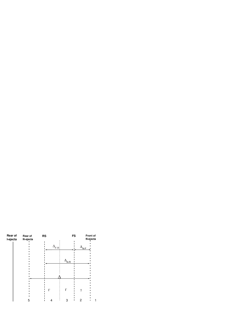
Figure 1.— A schematic diagram of a neutron-fed long GRB in the wind interaction case.

As shown in Figure 1, there are five regions: (1) the rest wind medium; (2) the unshocked neutron trail, moving with a LF $\gamma$; (3) the shocked neutron trail, moving with a LF $\Gamma$; (4) the shocked I-ejecta, moving with the LF $\Gamma$; and (5) the unshocked I-ejecta, moving with a LF $\Gamma_{\rm I}$. Notice we have generally defined the last LF as $\Gamma_{\rm I}$ rather than $\Gamma_{\rm I}^{0}$ since the decay products directly deposited onto the I-ejecta would change $\Gamma_{\rm I}$ from its initial value.

We first treat the dynamics of the neutron trail. The main purpose is to calculate the velocity of the mixture of the ambient particles with decay products (i.e. the trail) $\beta(R)=v(R)/c$. Following B03, we take $dm$, $|dM_{\rm n}|$ as the mass of the ambient medium overtaken by the N-ejecta and the mass of the decayed fast neutrons, respectively. For the long bursts we are discussing, only a fraction of $|dM_{\rm n}|$ is deposited onto the medium (the rest is deposited onto the I-ejecta). A shock propagates into the trail, and in the problem what is relevant is the fraction of the decay products that are deposited onto the unshocked trail (region 2 in Figure 1). We denote this fraction as

$$f\equiv\min\{1,~{}{\Delta_{\rm N-F}\over\Delta}\},$$ (5)

where $\Delta$ is the width of the N-ejecta, which is the same as that of the I-ejecta, and $\Delta_{\rm N-F}$ is the separation between the front of the N-ejecta and the front of the FS that propagates into the neutron decay trail. This is valid for the wind case, in which $\Delta_{\rm N-F}>0$ is always satisfied. For the ISM case (§3.2), under certain conditions the FS front leads the N-ejecta front, and we take $\Delta_{\rm N-F}<0$ following the same definition here. If this happens, nothing is deposited onto the unshocked medium, and in our treatment we will define $f=0$ whenever $\Delta_{\rm N-F}<0$ is satisfied. Notice that by defining $f$, we have assumed that neutrons in the N-ejecta decay uniformly within the length $\Delta$, which is justified by the fact $\Delta\ll R$. The same applies to the other two fraction parameters ($g$, eq.[16] and $h$, eq.[43] defined below).

The width $\Delta_{\rm N-F}$ is determined by

$$d\Delta_{\rm N-F}=(\beta_{\Gamma_{\rm n}}-\beta_{\Gamma_{\rm FS}})dR,$$ (6)

where $\Gamma_{\rm FS}$ is the LF of the FS and hereafter we denote $\beta_{\rm\Gamma_{\rm A}}$ as the dimensionless velocity corresponding to the LF $\Gamma_{\rm A}$.

Considering an inelastic collision between the medium (with mass $dm$) and the decay products (with mass $f|dM_{\rm n}|$), energy and momentum conservations give

$$f\Gamma_{\rm n}|dM_{\rm n}|+dm = \gamma(\gamma_{\rm th}+1)(dm+f|dM_{\rm n}|),$$

$$f\Gamma_{\rm n}\beta_{\Gamma_{\rm n}}|dM_{\rm n}| = \gamma\beta_{\gamma}(\gamma_{\rm th}+1)(dm+f|dM_{\rm n}|)~{},$$ (7)

where $\gamma_{\rm th}$ is the thermal LF of the mixture (exclude the rest mass). With equations (7), we have (see also B03)

$$\beta_{\gamma}(R)={\beta_{\rm\Gamma_{\rm n}}\over 1+(\Gamma_{\rm n}\zeta)^{-1}},~{}~{}\gamma(R)={\Gamma_{\rm n}\zeta+1\over(\zeta^{2}+2\Gamma_{\rm n}\zeta+1)^{1/2}};$$ (8)

where we have defined a parameter

$$\zeta(R) \equiv f{|dM_{\rm n}(R)|\over dm(R)}=f{M_{\rm n}\over R_{\rm\beta}}({dm\over dR})^{-1}$$ (9)

$$= {fM_{\rm n}^{0}\over km_{\beta}}({R\over R_{\beta}})^{\rm 1-k}\exp({-{R\over R_{\beta}}}),$$

which denotes the deposited neutron mass on unit medium mass (notice that it is slightly different from the same parameter defined in B03 with the correction introduced by the $f$ factor). Here $m_{\beta}$ is the mass of the medium contained within $R<R_{\beta}$, and $k$ is a parameter denoting the type of the medium, i.e. $k=1$ for the wind case and $k=3$ for the ISM case. For the wind case discussed here, we have

$$[\zeta(R)]^{\rm wind}={fM_{\rm n}^{0}\over m_{\beta}}\exp({-{R\over R_{\beta}}}).$$ (10)

Equations (7) also yields the initial thermal LF of the neutron trail

$$\gamma_{\rm th}=(\zeta^{2}+2\Gamma_{\rm n}\zeta+1)^{1/2}/(1+\zeta)-1.$$ (11)

For $\Gamma_{\rm n}^{-1}\ll\zeta\ll\Gamma_{\rm n}$ (which is valid for the wind case), the internal energy of the trail far exceeds its rest mass energy, i.e., $\gamma_{\rm th}\gg 1$, so that significant radiation is expected. When $\zeta>\Gamma_{\rm n}$ (e.g. the ISM case), one has $\gamma_{\rm th}\ll 1$ so that the trail emission is unimportant.

The total proton number density (in its proper frame) in the unshocked trail, including the neutron decay products, can be expressed as (B03)

$$n_{\rm tr}=n(1+\zeta)(\zeta^{2}+2\Gamma_{\rm n}\zeta+1)^{1/2}.$$ (12)

We define $\Delta_{\rm F-R}$ as the width of the shocked regions, i.e. the distance between the FS and the RS. One then has

$$d\Delta_{\rm F-R}=(\beta_{\rm\Gamma_{\rm FS}}-\beta_{\rm\Gamma_{\rm RS}})dR,$$ (13)

where $\beta_{\rm\Gamma_{\rm FS}}$ and $\beta_{\rm\Gamma_{\rm RS}}$ are the dimensionless velocities of the FS and the RS, respectively, which read (e.g., Sari & Piran 1995; Fan et al. 2004b)

$$\beta_{\rm\Gamma_{\rm FS}} \approx {\Gamma\beta_{\rm\Gamma}(4\gamma_{23}+3)-\gamma\beta_{\gamma}\over\Gamma(4\gamma_{23}+3)-\gamma},$$

$$\beta_{\rm\Gamma_{\rm RS}} \approx {\Gamma\beta_{\rm\Gamma}(4\gamma_{45}+3)-\Gamma_{\rm I}\beta_{\Gamma_{\rm I}}\over\Gamma(4\gamma_{45}+3)-\Gamma_{\rm I}},$$ (14)

where $\gamma_{23}$ is the LF of the region 2 relative to the region 3, and $\gamma_{45}$ is the LF of the region 5 relative to the region 4. They are calculated as

$$\gamma_{23}=\gamma\Gamma(1-\beta_{\gamma}\beta_{\rm\Gamma}),~{}~{}~{}~{}\gamma_{45}=\Gamma_{\rm I}\Gamma(1-\beta_{\rm\Gamma_{\rm I}}\beta_{\rm\Gamma}).$$ (15)

We define another fractional parameter $g$ as the fraction of the decay products that are deposited onto the shocked region (both regions 3 and 4 in Figure 1). We then have

$$g\equiv\left\{\begin{array}[]{@{\,}lc}{\Delta_{\rm F-R}}/{\Delta},&\mbox{for}~{}\Delta_{\rm N-R}<\Delta\\ 1-f,&\mbox{for}~{}\Delta_{\rm N-R}>\Delta\end{array}\right.~{},$$ (16)

where $\Delta_{\rm N-R}$ is the separation between the front of the N-ejecta and the RS front, which is described by

$$d\Delta_{\rm N-R}=(\beta_{\Gamma_{\rm n}}-\beta_{\rm\Gamma_{\rm RS}})dR.$$ (17)

When $\Delta_{\rm N-R}<\Delta$ the RS has not passed the end of the N-ejecta, while when $\Delta_{\rm N-R}>\Delta$, the RS passes through the end of the N-ejecta, reaching the region where no neutron decay product is being deposited.

For $\Delta_{\rm N-R}<\Delta$, some decay products are being deposited onto the I-ejecta directly (region 5 in Fig.1), which will alter the dynamics of the I-ejecta. We can treat the process in the way similar to the treatment of the neutron trail onto the circumburst medium. The difference here is that the I-ejecta itself is highly relativistic. The energy and momentum conservations are more analogous to those to describe internal shock collisions. Unlike the circumburst medium case in which the trail LF only depends on $R$, one needs two parameters to describe the I-ejecta dynamics. Besides the radius $R$, one needs to specify the location of the I-ejecta element in the I-ejecta proper. We parameterize this by the distance from the initial I-ejecta front, which is denoted as $\Delta_{1}$ so that $0<\Delta_{1}<\Delta$ is satisfied. After some algebra, the LF of the I-ejecta layer with the coordinate $\Delta_{1}$ at a particular $R$ could be written as

$$\Gamma_{\rm I}(\Delta_{1},R)=\sqrt{{\bar{\zeta}\Gamma_{\rm n}+(1+\gamma_{\rm th,I}^{0})\Gamma_{\rm I}^{0}\over\bar{\zeta}/\Gamma_{\rm n}+(1+\gamma_{\rm th,I}^{0})/\Gamma_{\rm I}^{0}}},$$ (18)

and the corresponding thermal LF reads

$$\gamma_{\rm th,I}(\Delta_{1},R)=\sqrt{{(\bar{\zeta}\Gamma_{\rm n}+\Gamma_{\rm I}^{0})[\bar{\zeta}/\Gamma_{\rm n}+(1+\gamma_{\rm th,I}^{0})/\Gamma_{\rm I}^{0}]\over(1+\bar{\zeta})^{2}}}-1,$$ (19)

where

$$\bar{\zeta}=\bar{\zeta}(\Delta_{1},R)\equiv\frac{M_{\rm n}^{0}}{M_{\rm I}^{0}}\left[1-\exp\left(-\frac{R_{1}}{R_{\beta}}\right)\right],$$ (20)

and $M_{\rm I}^{0}$ is the initial mass of the I-ejecta. The parameter $\bar{\zeta}$ is analogous to the $\zeta$ parameter (eq.[9]) for the trail treatment, which denotes the average decayed neutron mass on unit I-ejecta mass. The characteristic radius $R_{1}$ depends on whether or not the I-ejecta layer (with coordinate $\Delta_{1}$) overlaps the N-ejecta as the reverse shock sweeps the layer (so that the layer no longer belongs to the region 5). If the layer still overlaps with the N-ejecta as it is swept by the RS, through out the period when the layer is in the region 5 there has been always neutron decay products deposited onto the layer. In such a case, one simply has $R_{1}=R$. For those layers that the end of the N-ejecta has passed over earlier so that there is no neutron decay deposition at the RS sweeping time, one has to record the decayed neutron amount at the final moment with N-ejecta overlap. In this case, one has $R_{1}\approx 2(\Gamma_{\rm I}^{0}\Gamma_{\rm n})^{2}(\Delta-\Delta_{1})/(\Gamma_{\rm n}^{2}-{\Gamma_{\rm I}^{0}}^{2})$.

The RS crossing radius $R_{\times}$ can be calculated according to

$$\int^{R_{\times}}_{0}d\Delta_{\rm I-R}=\Delta,$$ (21)

where $\Delta_{\rm I-R}$ is the distance between the I-ejecta front and the RS assuming no shock compression. It is determined by

$$d\Delta_{\rm I-R}=(\beta_{\rm\Gamma_{\rm I}}-\beta_{\rm\Gamma_{\rm RS}})dR.$$ (22)

With the above preparation, one can delineate the dynamical evolution of the system for $R<R_{\times}$ using the following equations. After some algebra, the energy conservation of the system yields

$$(M+U/c^{2})d\Gamma=(\gamma-\Gamma\gamma_{23})(1+\gamma_{\rm th})dm_{\rm tr}+(\Gamma_{\rm I}$$

$$-\Gamma\gamma_{45})(1+\bar{\zeta})(1+\gamma_{\rm th,I})dm_{\rm I}+g(\Gamma_{\rm n}-\Gamma)|dM_{\rm n}|,$$ (23)

in deriving which, the small thermal energy generated by the deposition of the neutron decay products into the shocked region has been neglected. Here $U$ is the thermal energy generated in the two shock fronts, which can be calculated by

$$dU/c^{2} = (1-\epsilon_{1})[\gamma_{23}(1+\gamma_{\rm th})-1]dm_{\rm tr}$$ (24)

$$+ (1-\epsilon_{2})(1+\bar{\zeta})[\gamma_{45}(1+\gamma_{\rm th,I})-1]dm_{\rm I},$$

where $\epsilon_{1}$ and $\epsilon_{2}$ are the radiation efficiency (see the Appendix A for definition). The differential increase of the trail mass, the I-ejecta mass (just initially) and the total mass in the shock region can be expressed as

$$dm_{\rm tr} = [1+\zeta(R)]4\pi nR^{2}dR,$$ (25)

$$dm_{\rm I} = M_{\rm I}^{0}d\Delta_{\rm I-R}/\Delta,$$ (26)

$$dM = dm_{\rm tr}+(1+\bar{\zeta})dm_{\rm I}+g|dM_{\rm n}|,$$ (27)

Combining equations (13-27) with the well known radius–time relation

$$dR=\beta_{\rm\Gamma_{\rm FS}}c~{}dt/(1-\beta_{\rm\Gamma_{\rm FS}}),$$ (28)

one can calculate the dynamical evolution for $R<R_{\times}$ (see our numerical example in §3.1.4). Hereafter $t=t_{\rm obs}/(1+z)$ denotes the observer’s time corrected for the cosmological time dilation.

3.1.2 The dynamical evolution for $R>R_{\times}$

After the RS crosses the I-ejecta, only the FS exists. Equations (23, 24, 27) can be simplified as

$$(M+U/c^{2})d\Gamma=(\gamma-\Gamma\gamma_{23})(1+\gamma_{\rm th})dm_{\rm tr}+g(\Gamma_{\rm n}-\Gamma)d|M_{\rm n}|,$$ (29)

$$dU/c^{2}=(1-\epsilon_{1})[\gamma_{23}(1+\gamma_{\rm th})-1]dm_{\rm tr},$$ (30)

$$dM=dm_{\rm tr}+g|dM_{\rm n}|.$$ (31)

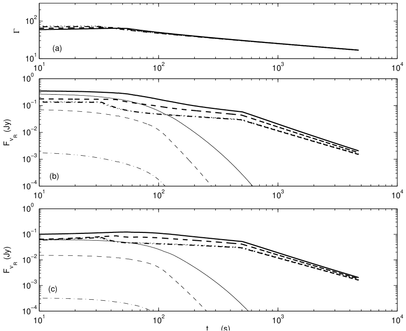
Figure 2.— The early optical afterglow lightcurves of a neutron-fed long GRB in the wind interaction case. (a) The dynamical evolution of the LF of the shocked region as a function of time. (b) R-band lightcurves, with the IC cooling effect due to the prompt $\gamma-$rays interacting with the shocked regions being ignored. Thick lines include contributions from all emission components, including the FS, RS and the neutron decay trail. Thin lines are for trail emission only (for a power-law energy distribution of the electrons, see Appendix B for details). The dotted, dash-dotted, dashed and solid lines represent $\chi=0.0,~{}0.1,~{}0.5,~{}1.0$ respectively. Following input parameters are adopted in the calculations: $E_{\rm tot}=2.0\times 10^{53}{\rm ergs}$, $\Delta=10^{12}$cm, $z=1$ [i.e. $D_{\rm L}=2.2\times 10^{28}{\rm cm}$, which corresponds to the standard $(\Omega_{m},\Omega_{\Lambda})=(0.3,0.7)$ $\Lambda$CDM cosmological model], $\Gamma_{\rm n}=300$, $\Gamma_{\rm m}=200$, $\Gamma_{\rm s,n}=30$, and $n=10^{35}{\rm cm^{-3}}R^{-2}$ (i.e. $A_{*}=1/3$), respectively. The parameters $\epsilon_{\rm e}=0.1$, $\epsilon_{\rm B}=0.01$ and $p=2.3$ are adopted for the FS and RS shocks as well as the trail. (c) R-band lightcurves, but the IC cooling effect due to the prompt $\gamma-$rays overlapping with the shocked region and the trail has been taken into account. The averaged $\gamma-$ray luminosity is taken as $L_{\gamma}=10^{51}{\rm ergs}~{}{\rm s}^{-1}$. Other parameters and line styles are the same as those in (b).

3.1.3 The impact of the initial prompt $\gamma-$rays on electron cooling

As pointed out by Beloborodov (2005), if the RS emission overlaps with the initial prompt $\gamma-$ray emission, the cooling of the shocked electrons is likely dominated by the inverse Compton (IC) scattering off the initial prompt $\gamma-$rays. This is a very common case for the wind-interaction case, as has been studied in detail in Fan et al. (2005a), who discuss the interesting sub-GeV photon emission and high energy neutrino emission due to the overlapping effect. In the ISM case, usually the prompt $\gamma-$ray emission has crossed the RS region before the RS emission becomes important, so that the above overlapping effect is not as important as in the wind model. We have performed calculations of the overlapping effect in the ISM model as well, and found that the resulted early optical afterglow lightcurves are nearly unchanged for typical parameters. So we do not present the result in Figure 5. Nonetheless, we would like to point out that for some GRBs born in the ISM environment whose duration is long enough and/or whose bulk LF is large enough, the overlapping effect should be also very important. This has been the case of GRB 990123 (Beloborodov 2005), which has a long ($T_{90}\sim 120{\rm s}$) duration and a large LF ($\sim 1000$).

Similar to Fan et al. (2005a), we assume that the internal shock efficiency is $r\simeq 0.2$ and define the IC cooling parameter $Y_{\rm s}\equiv U_{\rm\gamma}/U_{\rm B}$. Here $U_{\gamma}\simeq L_{\gamma}/4\pi R^{2}\Gamma^{2}c$ is the MeV photon energy density in the rest frame of the shocked region, and $U_{\rm B}=B^{2}/8\pi\simeq(\Gamma_{\rm I}^{0}/\Gamma)^{2}\epsilon_{B}n_{4}m_{p}c^{2}$ is the co-moving magnetic energy density in the same region, where $L_{\gamma}\simeq rcE_{\rm tot}/(1-r)\Delta$ is the luminosity of the $\gamma-$ray burst, and $n_{4}\approx E_{\rm tot}/4\pi R^{2}{\Gamma_{\rm I}^{0}}^{2}m_{\rm p}c^{2}\Delta$ is the co-moving density of the un-shocked ejecta. After some simple algebra, we derive $Y_{\rm s}\approx r/[(1-r)\epsilon_{\rm B}]$. Notice that this is only valid when the Klein-Nishina correction is unimportant, i.e. $x\ll 1$, where $x\equiv\epsilon_{\gamma}\gamma_{\rm e}/\Gamma m_{\rm e}c^{2}\sim\gamma_{\rm e}/\Gamma$, $\epsilon_{\gamma}\sim m_{\rm e}c^{2}$ is the energy of the prompt $\gamma-$rays, $\gamma_{\rm e}$ is the random LF of the emitting electrons. More generally, we should make the Klein-Nishina cross section correction, i.e. $\sigma_{\rm IC}=A(x)\sigma_{\rm T}$, where $A(x)\equiv{3\over 4}[{1+x\over x^{3}}\{{2x(1+x)\over 1+2x}-{\rm ln}(1+2x)\}+{1\over 2x}{\rm ln}(1+2x)-{1+3x\over(1+2x)^{2}}]$, with the asymptotic limits $A(x)\approx 1-2x+{26x^{2}\over 5}$ for $x\ll 1$, and $A(x)\approx{3\over 8}x^{-1}({\rm ln}2x+{1\over 2})$ for $x\gg 1$ (e.g. Rybicki & Lightman 1979). Notice that such a correction is necessary since the target photons, i.e. the initial prompt $\gamma-$rays are usually energetic enough in the rest frame of the electrons. As a result, for the electrons accelerated by the reverse shock, for $x\gg 1$, the Compton parameter reads (see Footnote 1 of Fan et al. [2005a] for derivation)

$$Y_{s}\approx{A(x)r\over x(1-r)\epsilon_{B}}$$ (32)

Usually, the magnetic field densities in the FS and the RS are nearly the same (e.g. Sari & Piran 1995), so Eq. (32) also applies to the FS shock region. The overlapping of the initial prompt $\gamma-$rays with the FS emission lasts until $\int{(1-\beta_{\rm FS})dR}=\Delta$.

Similarly, for the electrons accelerated in the neutron trail, we can also introduced the IC cooling parameter $Y_{T}\approx A(x_{1})U_{\gamma,T}/(x_{1}U_{B^{\prime}_{\rm tr}})$ for $x_{1}\gg 1$, where $U_{\rm\gamma,T}\approx L_{\gamma}/4\pi R^{2}\gamma^{2}c$, $B^{\prime}_{\rm tr}$ is calculated by Eq. (B1), and $x_{1}\equiv\epsilon_{\gamma}\gamma_{\rm e}/\gamma m_{\rm e}c^{2}\sim\gamma_{\rm e}/\gamma$.

When the prompt $\gamma-$rays overlap the shocked regions and the trail, to calculate the cooling frequency, the $Y$ parameter in Eqs. (A3), (B3) and (B4) should be replaced by $Y_{\rm s}$ (for electrons accelerated from the shock) or $Y_{\rm T}$ (for electrons accelerated in the neutron trail).

3.1.4 Model lightcurves

In Figure 2 we present the dynamical evolution of the system (Figure 2(a)) and the early optical afterglow lightcurves in Figs.2(b) and (c). In Fig.2(b) the IC cooling effect due to the initial prompt $\gamma-$ray overlapping with the shocked region and the trail has been ignored. In Fig.2(c), this IC cooling contribution is explicitly taken into account. The neutron-to-proton number density ratio $\chi$ is adopted as $\chi=0.0,0.1,0.5$ and 1, respectively.

As shown in Fig.2(a), for $R<R_{\times}$, $\Gamma$ is nearly a constant. This is consistent with the familiar result in the neutron-free wind model (e.g., Chevalier & Li 2000; Wu et al. 2003; Kobayashi & Zhang 2003b; Fan et al. 2004b; Yan & Wei 2005; Zou et al. 2005). The main reason is that the density of the N-ejecta also drops as $\propto R^{-2}$, and that the fraction of the decayed neutrons essentially remains the same during the shock crossing process. The latter effect is manifested by the fact that $R_{\times}$ is comparable to $R_{\beta}$ for the current nominal parameters, so that the neutron decay rate [$\propto\exp(-R/R_{\beta})$] remains essentially the same for $R<R_{\times}$.

The dynamical evolution of the shocks presented here [e.g. Fig.2(a)] look different from the one presented in Fig.1 of B03, which shows that the dynamics of a neutron-fed fireball is very different from the neutron-free one. This is because B03 presented the dynamical evolution of the trail in the radiative regime, i.e., the total thermal energy of the trail is radiated promptly before the trail is picked up by the I-ejecta. Here we assume an electron equipartition parameter $\epsilon_{\rm e}=0.1$ in the neutron trail. For such a small $\epsilon_{\rm e}$, even in the fast cooling regime, only 0.1 of the total thermal energy is radiated, and the system could be still approximated as an adiabatic one. Our results indicate that as long as the trail is in the quasi-adiabatic regime, the bulk of the energy is still dissipated in shocks, and the existence of the neutrons does not influence the dynamical evolution of the system significantly (see also B03 for similar discussions).

In any case, we include the emission contribution from the neutron trail by assuming a power-law distribution of the electrons, and find that it gives an interesting signature when $\chi$ is close to unity. In Fig.2(b) we present the lightcurves for different $\chi$ values, with the IC cooling by the initial prompt $\gamma-$rays ignored. The thick lines are the synthesized lightcurves including the contributions from the FS, RS and the neutron trail. In order to characterize the function of the trail, we plot the trail emission separately as thin lines. We can see that the early afterglow for $\chi=1$ shows a bright plateau lasting for $\sim 100$s, and the main contribution is from the trail. For $\chi\leq 0.5$, an early afterglow plateau with a shorter duration is still evident, but it is mainly due to the contribution of the RS emission. Comparing the lightcurves with small $\chi$’s (e.g. 0.0 and 0.1) to those with large $\chi$’s (e.g. 0.5 and 1.0), one can see that the early afterglow intensity is much stronger for high-$\chi$ case, although the dynamical evolution of the I-ejecta is rather similar [Fig.2(a)]. The reason is that the trail deposits an electron number density about 10 times of that in the wind medium, so that the total number of the emitting electrons in the shocked region is greatly increased.

In Fig.2(c) we present the lightcurves by taking into account the IC cooling effect due to the initial prompt $\gamma-$rays overlapping with the shocked regions and the trail. Line styles are the same as in Fig. 2(b). It is apparent that the very early R-band emission, including the FS emission, the RS emission and the trail emission, has been suppressed significantly. This means that the IC cooling effect is very essential in shaping the early afterglow lightcurves in the wind case. After the rear of initial prompt $\gamma-$ray front has crossed the FS front, the FS emission becomes rather similar to that of the Fig.2(b).

In the wind case, the difference between the neutron-rich lightcurve and a neutron-free lightcurve is only marginal (both Fig.2(b) and Fig.2(c)). One potential tool to diagnose the existence of the neutron component is to search for the trail emission component. This is in principle not straightforward since there are many uncertainties in categorizing the trail emission (Appendix B). In Figure 3 (with the IC cooling effect ignored), we calculate the expected trail emission for two extreme models for electron energy distribution, i.e. a power law model and a mono-energetic model. A more realistic model should lie in between these two models. Figure 3 indicates a fortunate fact that the differences between the two extreme models are far from large, although the mono-energetic model predicts a stronger R-band trail emission. This gives us confidence that the crude treatment of the trail emission in Fig.2 gives a first-order presentation of the reality. Another remark is that different electron energy distributions result in different trail emission spectrum. In particular, a mono-energetic or thermal-like distribution gives rise to a much lower emissivity at high frequencies. Even in the optical band, multi-color observations at early times can be used to diagnose the existence of the neutron trail. For example, if the trail electron energy distribution is thermal-like or in a form largely deviated from the simple power-law, multi-color observations around 100s with the UVOT on board Swift (there are 6 colors in the 170-650 nm band for UVOT) can reveal interesting clues of the existence of neutrons in the fireball.

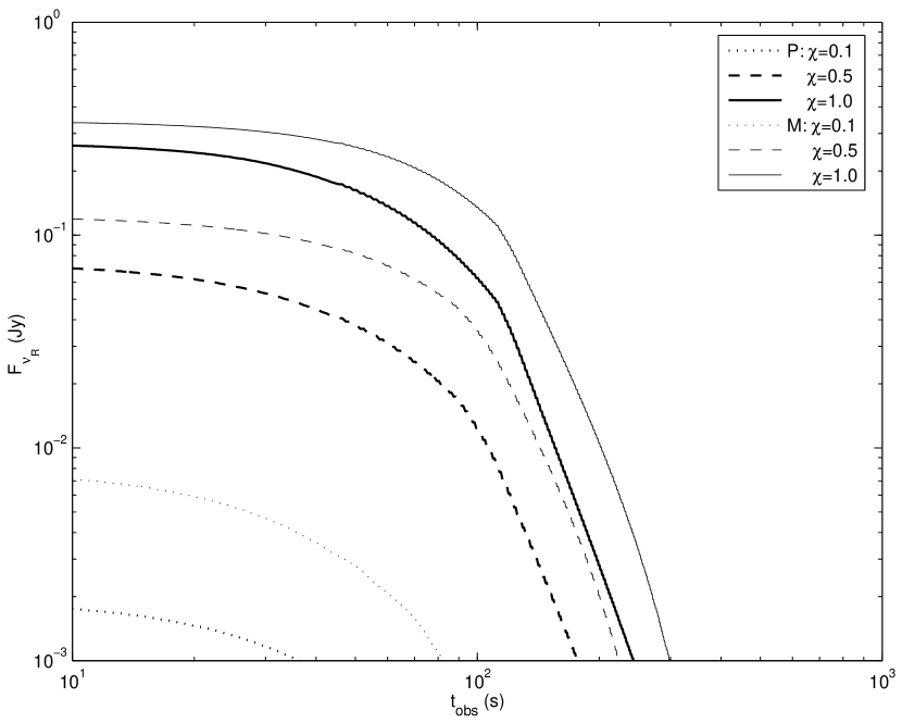
Figure 3.— The trail emission lightcurve in the wind interaction case, with the IC cooling effect due to the initial prompt $\gamma-$rays overlapping with the trail ignored. The dotted, dashed and solid lines represent $\chi=0.1,~{}0.5,~{}1.0$ respectively. The thick lines (marked by P) represent the emission by assuming a power law distribution of electrons, and thin lines (marked by M) represent the emission by assuming a mono-energetic distribution. The initial input parameters are the same as those presented in Figure 2(b) caption.

3.2. ISM case

We now turn to discuss the ISM-interaction for long GRBs. The main characteristic of the ISM case is that the trail typically moves faster than the I-ejecta, so that a gap forms between the I-ejecta and the T-ejecta (the trail ejecta). The latter interacts with the ISM and dominates the early afterglow. Later the I-ejecta catches up and produces an energy injection bump signature. Below we will calculate the typical lightcurves with the nominal parameters adopted in this paper. Two stages will be considered separately, i.e. (1) when the T-ejecta is separated from the I-ejecta and dominates the afterglow emission, and (2) when the I-ejecta collide onto the decelerated T-ejecta. Except otherwise stated, the notations adopted in this section are the same in §3.1 when the wind case is discussed.

3.2.1 The dynamical evolution of T-ejecta before I-ejecta collision

The $\zeta(R)$ parameter (eq.[9]) in the ISM case reads

$$[\zeta(R)]^{\rm ISM}={fM_{\rm n}^{0}\over 3m_{\beta}}({R\over R_{\beta}})^{-2}\exp({-{R\over R_{\beta}}}),$$ (33)

For $\chi=1$, the nominal parameters are $\Gamma_{\rm I}^{0}=100$, $\Gamma_{\rm n}=300$, $\gamma_{\rm th,I}^{0}=0.433$ and $\zeta(R)=2.85\times 10^{4}f(R/R_{\beta})^{-2}\exp(-R/R_{\beta})$. The N-ejecta leads the I-ejecta, and completely separates from the I-ejecta at

$$R_{\rm s}\simeq\frac{\Delta}{\beta_{\Gamma_{\rm n}}-\beta_{\Gamma_{\rm I}^{0}}}\simeq\frac{2{\Gamma_{\rm I}^{0}}^{2}\Gamma_{\rm n}^{2}\Delta}{(\Gamma_{\rm n}^{2}-{\Gamma_{\rm I}^{0}}^{2})}.$$ (34)

As long as $f\exp(-R/R_{\beta})(R/R_{\beta})^{-2}>2.34\times 10^{-3}$, one has $\gamma(R)>\Gamma_{\rm I}^{0}$ (eq.[8]). The I-ejecta lags behind the trail, and a gap forms between the I-ejecta and the trail. This happens for $\chi>{\rm several}~{}\times 0.1$, when the decay products deposited onto the ISM have a large enough momentum to drag the trail fast enough to lead the I-ejecta. With equation (34), we can estimate how many decay products have been deposited into the I-ejecta directly

$$M_{\rm n,d} \simeq M_{\rm n}^{0}\int_{0}^{\rm R_{\rm s}}(1-{R\over R_{\rm s}})\exp(-{R\over R_{\rm\beta}}){dR\over R_{\beta}}$$ (35)

$$= [1+{\exp({\rm-a})\over a}-{1\over a}]M_{\rm n}^{0},$$

where $a=R_{\rm s}/R_{\beta}$. For $a>2$, we have $M_{\rm n,d}>0.5M_{\rm n}^{0}$, i.e., most of decay products have been deposited into the I-ejecta.

For the trail, the layers from the behind moves faster than the leading layers, since $[\zeta(R)]^{\rm ISM}$ decreases with $R$. This leads to pile-up of the trail materials. The faster trail materials would shock into the slower trail materials in front. In the following treatment, we approximately divide the trail materials into two parts. The fast trail (including forward shocked trail) is denoted as the T-ejecta, while the upstream unshocked part is still called the trail. The location of the shock is roughly defined by requiring the bulk LF of the T-ejecta (which is calculated through energy and momentum conservation) is larger than $2\gamma$, so that the relative LF between the two parts exceeds 1.25. Since the trail is hot with a relativistic temperature, the upstream local sound speed $c/\sqrt{3}$ corresponds to a local sound LF $\simeq\sqrt{3/2}\sim 1.22$. So our shock forming condition is self-consistent. The shock front moves faster than the T-ejecta, and $\beta_{\rm\Gamma_{\rm FS}}$ may exceed $\beta_{\rm\Gamma_{\rm n}}$. If this persists long enough, the N-ejecta lags behind the FS front. The decay products deposit into the shocked material directly rather than mixing with the ISM. The shock propagates into the ISM directly. In such a case, the dynamics is simplified.

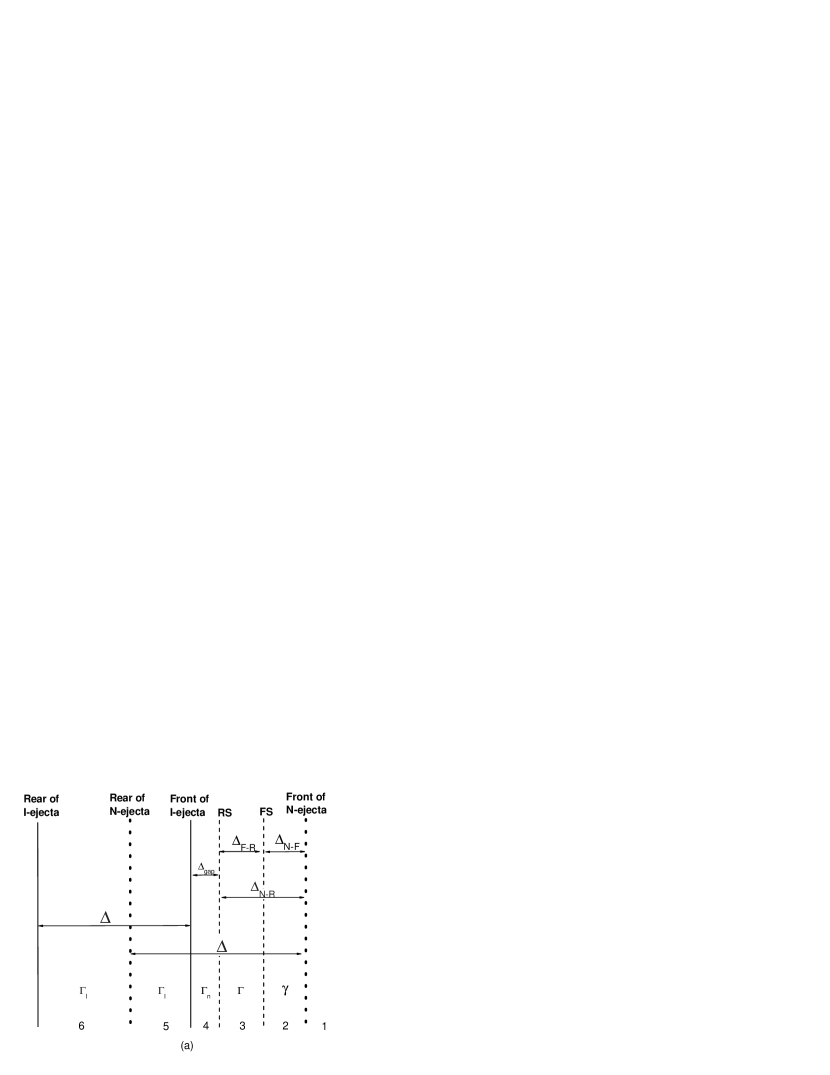
Figure 4.— The schematic diagram of a neutron-fed long GRB in the ISM-interaction case. (a) When the T-ejecta (region 3) is separated from the I-ejecta and interacts with the trail or ISM. (b) When the I-ejecta collides into the T-ejecta producing refreshed shocks.

Before collision, there are six regions in the whole system (see Fig.4(a) for illustration): (1) the rest ISM; (2) the unshocked trail moving with $\gamma$; (3) the T-ejecta (including the shocked trail between the FS and the RS) moving with $\Gamma$; (4) the gap between the T-ejecta rear and the I-ejecta front, in which the decayed protons move with $\sim\Gamma_{n}$; (5) the overlapped region of the I-ejecta and the N-ejecta; and (6) free moving I-ejecta.

The width of the T-ejecta (i.e., region 3), $\Delta_{\rm F-R}$ is still governed by equation (13), but now $\beta_{\Gamma_{\rm RS}}=[\Gamma\beta_{\Gamma}(4\gamma_{34}+3)-\Gamma_{\rm n}\beta_{\Gamma_{\rm n}}]/[\Gamma(4\gamma_{34}+3)-\Gamma_{\rm n}]$, where $\gamma_{34}=\Gamma\Gamma_{\rm n}(1-\beta_{\Gamma}\beta_{\Gamma_{\rm n}})$ is the LF of region 4 relative to region 3. The fraction of the decay products deposited into the T-ejecta directly, $g$, is still defined by equations (16) and (17), in which we take $f=\min\{1,\Delta_{\rm N-F}/\Delta\}$, and $f=0$ when $\Delta_{\rm N-F}$ is negative.

Energy conservation of the T-ejecta interacting with the regions 2 and 4 results in

$$(U/c^{2}+M)d\Gamma=(\gamma-\Gamma\gamma_{23})(1+\gamma_{\rm th})dm_{\rm tr}$$

$$+g(\Gamma_{\rm n}-\Gamma)|dM_{\rm n}|+(\Gamma_{\rm n}-\Gamma\gamma_{34})dm_{\rm gap},$$ (36)

where $U$ is the thermal energy generated in both the FS and RS fronts, which is described by

$$dU/c^{2} = (1-\epsilon_{1})[\gamma_{23}(1+\gamma_{\rm th})-1]dm_{\rm tr}$$ (37)

$$+ (1-\epsilon_{2})(\gamma_{34}-1)dm_{\rm gap},$$

$dm_{\rm gap}$ is the differential mass swept by the RS from the gap, which can be approximated by

$$dm_{\rm gap}=lM_{\rm gap}{d\Delta_{\rm N-R}\over\Delta_{\rm gap}},$$ (38)

where $l=1$ for $\Delta_{\rm N-R}\leq\Delta$ and $l=0$ otherwise (see equation (17) for the definition of $\Delta_{\rm N-R}$). This step function is used to characterize whether there is decay product falling into the gap region. $M_{\rm gap}$ is the total mass contained in the region (4), which satisfies

$$dM_{\rm gap}={l\Delta_{\rm gap}\over\Delta}|dM_{\rm n}|-dm_{\rm gap}.$$ (39)

The width of the gap $\Delta_{\rm gap}$ (i.e., the separation of the T-ejecta rear and the I-ejecta front), is governed by

$$d\Delta_{\rm gap}=\left\{\begin{array}[]{@{\,}lc}(\beta_{\Gamma_{\rm RS}}-\beta_{\Gamma_{\rm I}})dR,&\mbox{for}~{}\Delta_{\rm N-R}<\Delta,\\ (\beta_{\Gamma}-\beta_{\Gamma_{\rm I}})dR,&\mbox{for}~{}\Delta_{\rm N-R}>\Delta.\end{array}\right.$$ (40)

The total mass in the T-ejecta can be calculated through

$$dM=dm_{\rm tr}+g|dM_{\rm n}|+dm_{\rm gap},$$ (41)

where $dm_{\rm tr}$ is still defined by equation (25). Notice that the expression of $dm_{\rm tr}$ is reduced to $dm_{{}_{\rm ISM}}$ when $f=0$ is satisfied, i.e. there is no decay products deposited onto the unshocked medium. This usually does not happen in the wind case, but happens sometimes in the ISM case.

During this stage, the I-ejecta evolves independently. Because of the deposition of decay products, the I-ejecta is somewhat accelerated. To estimate this effect, we assume that the I-ejecta moves with a uniform LF $\Gamma_{\rm I}$. In principle, the part that overlaps with the N-ejecta (so that deposition of the decay products is possible) should move slightly faster than the rest part, and within the decay-area different layers may move with slightly different LFs. But such an effect is unimportant for our further discussions about the interaction between the I-ejecta and the T-ejecta. Energy and momentum conservations then yield

$$(M_{1}+U_{1}/c^{2})d\Gamma_{\rm I}=[(\Gamma_{\rm n}-\Gamma_{\rm I})-\Gamma_{\rm I}(\gamma_{\rm rel}-1)]h|dM_{\rm n}|,$$ (42)

where

$$h=\max\{0,1-{\Delta_{\rm gap}+\Delta_{\rm F-R}+\Delta_{\rm N-F}\over\Delta}\},$$ (43)

and $\gamma_{\rm rel}=\Gamma_{\rm I}\Gamma_{\rm n}(1-\beta_{\Gamma_{\rm I}}\beta_{\Gamma_{\rm n}})$ is the relative LF between the N-ejecta and the I-ejecta, $U_{1}$ and $M_{1}$ are determined by $dU_{1}/c^{2}=(\gamma_{\rm rel}-1)h|dM_{\rm n}|$ and $dM_{1}=h|dM_{\rm n}|$ (Originally, $M_{1}=M_{\rm I}^{0}$), respectively. We can then solve $\Gamma_{\rm I}$ at any time, which is adopted as the input parameter in the next section.

3.2.2 The collision between the I-ejecta and the T-ejecta

At the beginning of the evolution, one has $\Gamma>\Gamma_{\rm I}$, and the I-ejecta lags behind further and further. However, the T-ejecta is decelerated by the trail and the ISM continuously, so that $\Gamma$ decreases with radius. When $\Gamma=\Gamma_{\rm I}$ the separation between the I-ejecta and the T-ejecta is the largest. Later one has $\Gamma<\Gamma_{\rm I}$, and the gap between the two ejecta shrinks, until eventually the I-ejecta catches up with the T-ejecta. This is a standard energy injection process, and a pair of refreshed shocks are formed, i.e. a refreshed FS (RFS) expanding into the hot T-ejecta, and a refresh RS (RRS) penetrating into the I-ejecta. The detailed treatment of such a process has been presented before (e.g. Kumar & Piran 2000; Zhang & Mészáros 2002). In particular, Zhang & Mészáros (2002) considered the interactions between three media, i.e. the ISM, the initial fireball shell and an injected shell. They considered three emitting shocks, including the leading forward shock and the pair of the refreshed shocks. Their analysis is pertinent to treat the current problem. As shown in Zhang & Mészáros (2002), the emission powered by the RFS is unimportant in the optical band, (see the short dashed line in their Fig. 4b). Since we are mainly focused on the optical lightcurves in this paper, that result leads to great simplification of our treatment. In our calculations, only the RRS and the FS are taken into account. The simplified system includes 5 parts (see Figure 4(b) for illustration): (1) the unshocked ISM, (2) the unshocked trail (this region may merge to region 1), (3) T-ejecta and shocked trail, (4) shocked I-ejecta, and (5) unshocked I-ejecta. Notice that we no longer separate the unshocked I-ejecta into two regions (whether overlap with the N-ejecta), since we treat the unshocked I-ejecta as a whole with a same LF $\Gamma_{\rm I}$.

Energy conservation of the the system (T-ejecta, the shocked trail and the shocked I-ejecta) yields

$$(U_{2}/c^{2}+M_{2})d\Gamma=(\gamma-\Gamma\gamma_{23})(1+\gamma_{\rm th})dm_{\rm tr}$$

$$+(\Gamma_{\rm I}-\Gamma\gamma_{\rm 45})(1+\gamma_{\rm th,I})dm_{\rm I}+g(\Gamma_{\rm n}-\Gamma)|dM_{\rm n}|,$$ (44)

where $\gamma_{23}$ and $\gamma_{\rm 45}$ are the relative LFs between region 2 and 3, and region 4 and 5, respectively (eq.[15]), $U_{2}$ is the thermal energy generated in the shocks, which is determined by

$$dU_{2}/c^{2} = (1-\epsilon_{1})[(1+\gamma_{\rm th})\gamma_{23}-1]dm_{\rm tr}$$ (45)

$$+ (1-\epsilon_{2})[(1+\gamma_{\rm th,I})\gamma_{\rm 45}-1]dm_{\rm I},$$

and $M_{2}$ is the total mass in the shocked region

$$dM_{2}=dm_{\rm tr}+dm_{\rm I}+g|dM_{\rm n}|.$$ (46)

Here $\gamma_{\rm th,I}=U_{1}/M_{1}c^{2}$, $dm_{\rm I}\approx M_{1}d\Delta_{\rm I-R}/\Delta$, $d\Delta_{\rm I-R}=(\beta_{\Gamma_{\rm I}}-\beta_{\rm\Gamma_{\rm RS}})dR$ (eq.[22]), and $M_{1}$ is the total I-ejecta mass upon collision (according to eq.[42]). The velocity of the RRS reads $\beta_{\rm\Gamma_{\rm RS}}\approx[\Gamma\beta_{\rm\Gamma}(4\gamma_{\rm 45}+3)-\Gamma_{\rm I}\beta_{\rm\Gamma_{\rm I}}]/[\Gamma(4\gamma_{\rm 45}+3)-\Gamma_{\rm I}]$.

After the reverse shock crosses the I-ejecta, the I-ejecta and the T-ejecta merge into one single shell, and the influence of the neutron component essentially disappears. The later dynamical evolution of this merged shell is the same as that in the neutron-free model, which has been studied in many publications (e.g. Huang et al. 2000; Panaitescu & Kumar 2002). We do not discuss it further in this paper.

3.2.3 Model Lightcurves

The dynamical evolution of the system (LF of the T-ejecta) and the R-band lightcurve in the ISM-interaction case are calculated for $\chi=$0, 0.1, 0.5, 1.0, respectively (see Figure 5). In the cases of $\chi=0.5$ and $\chi=1$, there is a gap between the I-ejecta and the T-ejecta, and a bump is evident in both the $\Gamma-t_{\rm obs}$ and $F_{\nu_{\rm R}}-t_{\rm obs}$ diagrams. This bump is the signature for the I-ejecta and T-ejecta collision. When $\chi\leq 0.1$, this signature is not significant, mainly because the gap is not well-developed. The trail is picked up by the I-ejecta continuously, so that the treatment is similar to the one to calculate the wind case (see §3.1). The R-band lightcurve for $\chi=0.1$ is rather similar to the $\chi=0$ case, except that it is relatively brighter at earlier times (e.g. before the RS crosses the I-ejecta). The reason is that even in the $\chi=0.1$ case, the trail is much denser than the ISM, so that there are more electrons in the forward shock front that contribute to synchrotron radiation. The early R-band flux for $\chi=0.5$ and $\chi=1$ is also different from the case of $\chi=0$. This is because the early afterglow for a high-$\chi$ case is powered by the T-ejecta, which has a smaller mass in the beginning than the I-ejecta. The T-ejecta soon enters the deceleration phase, so that $\Gamma$ starts to drop with time at a very early epoch (see Figure 5(a)). In our calculation, it is found out that for high-$\chi$ case, the initial RS that crosses the T-ejecta is too weak for any observational consequence. For a comparison, for the low-$\chi$ case ($\chi\leq 0.1$), the more massive I-ejecta is decelerated slowly, and it is not significantly decelerated within 100 seconds (see Figure 5(a)). In the meantime, a strong RS crosses the I-ejecta, whose emission is included in our calculations. This keeps a higher level of the early afterglow emission. In all the cases, the rising behavior of the early afterglow is because the typical synchrotron frequency is above the band. For the high-$\chi$ case, the obvious bump signature is the joint contribution from the FS and the RRS, and latter is the dominant component in the optical band. For illustrative purpose, in Figure 5(b), besides the total lightcurve, we also plotted the RRS contribution in the $\chi=1.0$ case, and the initial RS contribution in the $\chi=0.0$ case.

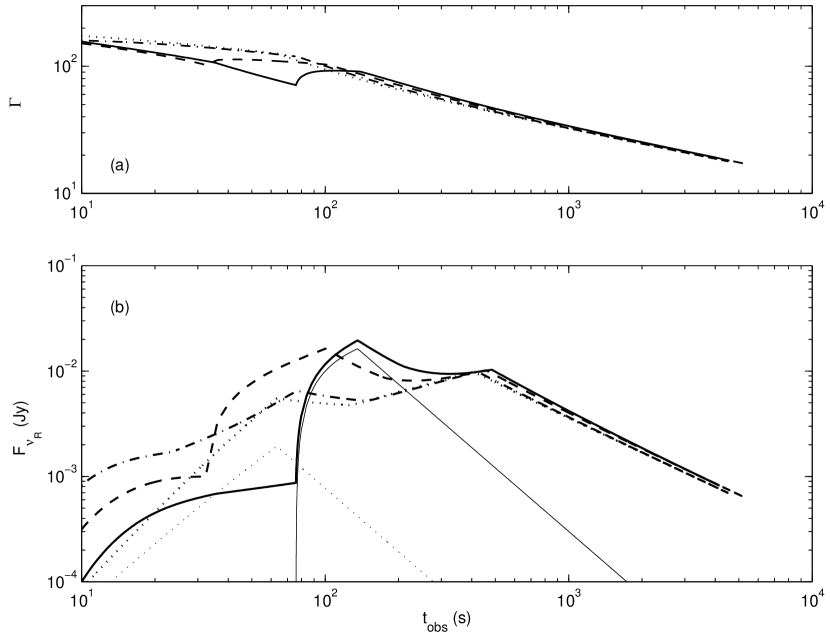
Figure 5.— The early optical afterglow lightcurves of a neutron-fed long GRB in the ISM interaction case. (a) The dynamical evolution of the region shocked by FS as a function of time. The dotted, dash-dotted, dashed, and solid lines represent $\chi=0.0,~{}0.1,~{}0.5,~{}1.0$ respectively. (b) R-band lightcurves. Line styles are the same as in (a). Thick lines represent the total early R-band lightcurves, while the thin lines are for RS emission only. For clarity, only the RS emission for $\chi=0$ and the RRS emission for $\chi=1$ cases are plotted. The initial parameters are the same as those listed in the caption of Figure 2, except that $n=1{\rm cm^{-3}}$ is adopted.

An interesting question is to explore how to use the lightcurve to diagnose the existence of the neutron component for the ISM case. For example, the initial rising lightcurve of a neutron-free fireball is steep, while for a neutron-fed fireball it is much milder because of the contribution of the shocked trail emission. The sharp bump in the early afterglow stage is a prominent signature. However, it suggests that an energy injection event happens, not necessarily a proof of the existence of the neutron component. Nonetheless, the neutron-fed model gives a natural mechanism for post energy injection, and it suggests that an early bump is common for long GRBs with ISM-interaction as long as $\chi$ is reasonably large, say $>0.5$. If future Swift observations reveal that an early bump is common, it may suggest that the GRB fireballs are baryonic with a large fraction of neutrons. It is worth mentioning that for the neutron-free model, an early afterglow bump is also expected due to the transition from the RS emission to the FS emission (e.g. Kobayashi & Zhang 2003a; Zhang et al. 2003). Nonetheless, the bump due to energy injection (presumably powered by the collision between the I-ejecta and the T-ejecta) could be well-differentiated. For example, the injection bump is achromatic, while the FS peak is chromatic, caused by crossing of the typical frequency into the band. Finally, the RS emission for $\chi=0$ is weaker than the RRS emission in the high-$\chi$ case (Figure 5(b)). This is because the ejecta is assumed to be cold for the neutron-free case, while for the neutron-rich case, it is hot (see equation (2)). At the RRS front, the original thermal energy of the protons would be also shared by the electrons, leading to stronger emission.

The neutron-fed signatures last only for a few 100 seconds. Rapid and frequent monitoring (e.g. with $\sim$ 5 s exposure interval) of early optical afterglow is needed to catch these signatures. Swift UVOT, with an on-target time 60-100 s, has the capability to detect such signals.

4. Early optical afterglow lightcurves: short GRBs

Bursts with durations shorter than 2 s may have different physical origin. The leading model for short GRBs invokes mergers of two compact objects (e.g., NS-NS merger or BH-NS merger, see e.g. Eichler et al. 1989). Although there are other suggestions about the origin of short GRBs, the merger model was found suitable to interpret many short GRB properties (e.g. Ruffert et al. 1997). A pre-concept of such a merger model is that the burst site is expected to have a large offset from the host galaxy due to asymmetric kicks during the births of the NSs, and that the number density of the external medium is low, typically $0.01{\rm cm^{-3}}$. Such a suggestion seems to receive support from the afterglow data of the recent short, soft GRB 040924 (Fan et al. 2005b). As already mentioned in the introduction, in the compact object merger model (especially the NS-NS merger model), the outflow is very likely to be neutron-rich ($\chi\geq 1$). Here we calculate the early optical afterglow lightcurve of a neutron-rich short GRB ($\chi=1$) and compare it with the neutron-free case.

We take the following typical parameters for a short GRB. The burst duration is taken $\sim 0.2{\rm s}$, so that the width of the N-ejecta is $\Delta\sim 6\times 10^{9}{\rm cm}$. The total (include both protons and neutrons) isotropic energy is $E_{\rm tot}=2.0\times 10^{51}{\rm ergs}$. The initial LF of the merged ion shell and the neutron shell are $\Gamma_{\rm m}=200$, $\Gamma_{\rm n}=300$, respectively. The I-eject and the N-ejecta separate at a radius $\approx 2\Gamma_{\rm m}^{2}\Gamma_{\rm n}^{2}\Delta/(\Gamma_{\rm n}^{2}-\Gamma_{\rm m}^{2})\approx 10^{15}{\rm cm}$, which is much smaller than the typical decay radius $\simeq 8\times 10^{15}{\rm cm}$. As a result, for short bursts most of the neutron decay products are deposited onto the ISM (i.e. $f\sim 1$). This is the “clean” scenario discussed by B03. The resulting $\zeta(R)$ in the trail is very large for $R\sim{\rm several}~{}R_{\beta}$, and a gap still forms between the trail (T-ejecta) and the I-ejecta. The calculation is therefore the same as the ISM-model for long GRBs (see §3.2 for detail). For $\Delta\sim 10^{10}{\rm cm}$ and $\Gamma_{\rm m}\sim 200$, the I-ejecta starts to spread at $R>10^{15}{\rm cm}$ (e.g., Piran 1999). This radius is much smaller than the deceleration radius, which is $\simeq 7\times 10^{16}E_{\rm tot,51}^{1/3}n_{-2}^{-1/3}\Gamma_{\rm m,2.3}^{-2/3}{\rm cm}$ for $\chi=0$. In our calculation, we take the spreaded width $\sim 5\times 10^{11}{\rm cm}$ when calculating the RS emission. Also here we perform numerical calculations as compared with the analytical treatment presented in Fan et al. (2005b). We found that the relative LF between the unshocked I-ejecta and the shocked I-ejecta is smaller than the one estimated in Fan et al. (2005b), so that the RS emission is further suppressed.

The lightcurves are plotted in figure 6 for $\chi=0$ and $\chi=1$. Similar to figure 5(b), the main difference between the two cases is that for the latter the very early lightcurve increases more slowly with time. This is due to the contribution from the shocked trail. A collision also happens as the I-ejecta catches up with the decelerated T-ejecta. The signature, which is manifested as a steeper increasing lightcurve around 20 s, is however not as prominent as the long GRB case. There are two reasons. One is that the T-ejecta and the I-ejecta now have a comparable mass, since essentially all the neutron decay products are stored in the T-ejecta (for comparison, for long bursts, a good fraction is deposited onto the I-ejecta so that the I-ejecta is much more energetic than the T-ejecta). Second, the RRS is very weak, and the main contribution to the lightcurve is the FS component (for comparison, for long bursts, the RRS component dominates the bump emission). Nonetheless, we identify some novel features of a neutron-rich short GRB. The signature occurs too early, however, and the global afterglow level is very dim due to the small $E_{\rm tot}$ and $n$. It is still a challenging task to diagnose the neutron component in short GRBs.

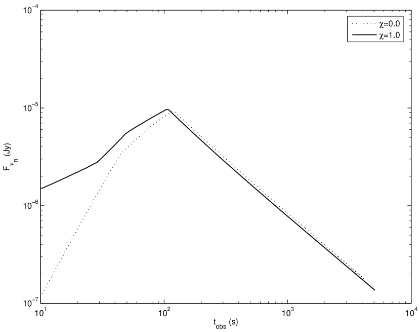
Figure 6.— Early R-Band lightcurves for a typical short GRB for $\chi=1$ (solid) and $\chi=0$ (dotted), respectively. The input parameters are the same as those listed in the caption of figure 2, except that $n=0.01{\rm cm^{-3}}$ and $E_{\rm tot}=2\times 10^{51}{\rm ergs}$ are adopted.

5. Discussion and summary

The composition of the outflow that powers GRBs is still far from clear. The well-collected late afterglow data are unfortunately not suitable to study the GRB fireball composition, since the afterglow radiation comes from the shocked medium rather than the fireball materials. Understanding the fireball composition and hence the nature of the explosion requires detailed early afterglow data. In general a GRB fireball is composed of two distinct components, a baryonic component and a Poynting flux component. Current early afterglow data suggest that GRB ejecta seem to be magnetized (e.g. Fan et al. 2002; Zhang et al. 2003; Kumar & Panaitescu 2003). Closer modeling suggests that for GRB 990123 and GRB 021211 in which the reverse shock magnetic field is stronger than that in the forward shock region, the $\sigma$ parameter, i.e. the Poynting flux to baryonic flux ratio, is moderate (Zhang & Kobayashi 2004; Fan et al. 2004b). In other two cases of early afterglow (GRB 021004 and GRB 030418), detailed modeling is needed to reveal whether Poynting flux is important. In any case, it is likely that the baryonic component is at least non-negligible. As discussed in the introduction, the neutron component is an inevitable composition within the baryonic component, and the diagnosis of the neutron component is a handle to reveal the significance of the baryonic component in GRB fireballs. In the literature, the possible neutron signatures discussed include the multi-GeV neutrino emission (e.g. Derishev et al. 1999a; Bachall & Mészáros 2000; Mészáros & Rees 2000) and the UV flash accompanying the $\gamma-$ray emission phase (Fan & Wei 2004) . The detection of these signals are difficult due to the limitation of the current detector capability.

The most prominent neutron signature is likely imprinted in the early afterglow. This suggestion has been proposed (e.g. Derishev et al. 1999b; B03), but no detailed calculations have been performed. In this paper, we present a first detailed calculation of early optical afterglow lightcurves for a neutron-fed fireball. We considered both long and short GRBs, and for long GRBs we consider both a ISM medium and a wind medium. For each model, we calculate the lightcurves for different $\chi$ (the neutron-to-proton number density ratio) values, aiming to study how the neutron component progressively change the lightcurve behavior as $\chi$ increases. We confirmed the previous suggestions that the presence of neutrons changes the fireball dynamics and the lightcurves (Derishev et al. 1999b; B03). Our findings are summarized as follows.

1. For short GRBs, the neutron decay products deposit onto the ISM medium mostly, and the neutron decay trail clearly separates from the ion ejecta (I-ejecta). This is the clean picture delineated in B03. For long GRBs, the picture is more complicated. Only part of the decay products are deposited onto the medium. The rest are deposited onto the I-ejecta itself or onto the shocked region. The neutron signatures in long GRBs therefore require more complicated treatments.

2. If the medium is a pre-stellar wind (for long GRBs), the neutron trail moves slowly (mainly because the medium inertia is too large). The trail and the I-ejecta do not separate from each other, and a forward shock propagates into the trail directly. Three components contribute to the final emission, i.e. the forward shock, the reverse shock propagates into the I-ejecta, and the unshocked trail emission. The latter is significant when $\chi$ is large, since the internal energy of the unshocked trail is large when the medium density is high. A typical neutron-rich wind-interaction lightcurve is a characterized by a prominent early plateau lasting for $\sim 100$ s followed by a normal power-law decay (Fig.2). We also show that in the wind case, the IC cooling effect due to the overlapping of the initial prompt $\gamma-$ray with the shocks and the trail (e.g. Beloborodov 2005; Fan et al. 2005a) suppresses the very early R-band afterglow significantly, and the neutron-fed signature is also dimmed (see Fig.2(b) and Fig.2(c) for a comparison).

3. If the medium is a constant density ISM (for long GRBs), part of the neutron decay products fall onto the medium, and the trail moves faster than the I-ejecta. A gap likely forms between the leading trail and the I-ejecta. The former forms a distinct trail ejecta (T-ejecta) which interacts with the out trail or ISM. The latter catches up later and gives rise to a rebrigtening signature. Before collision, the radiation is dominated by the forward shock emission. During the collision, both the forward shock emission and the refreshed shocks (especially the refreshed reverse shock) are important. The unshocked trail emission is not important in this case. A typical neutron-rich ISM-interaction lightcurve is characterized by a slow initial rising lightcurve followed by a prominent bump signature around tens to hundreds of seconds (Fig.5).

4. The picture for short GRBs is similar to the case of long GRBs with ISM-interaction. The injection bump is less prominent and the refreshed reverse shock is not important. A typical neutron-rich short GRB lightcurve is characterized by a slow initial rising lightcurve followed by a step-like injection signature (Fig.6).

For all the cases, the predicted signatures can be detected by the UVOT on board the Swift observatory. However, most of these signatures (such as the plateau and the bump signature) are not exclusively for neutron decay. More detailed modeling and case study are needed to verify the existence of the neutron component.

A neutron-fed fireball involves very complicated processes and some not well-studied physical problems (e.g. particle acceleration and emission in the trail). In principle a complicated numerical model is needed to delineate the problem. In this paper, we made some approximations to simplify the problem and eventually come up with a semi-analytical model. Such a treatment nonetheless catches the main novel features of the model. Further studies are needed to build up a more realistic model of neutron-fed fireballs.

So far there are four GRBs whose early afterglows are detected (Akerlof et al. 1999; Fox et al. 2003a, 2003b; W. Li et al. 2003; Rykoff et al. 2004, see Zhang & Mészáros 2004 for a recent review), i.e. GRB 990123, GRB 021004, GRB 021211 and GRB 030418. Modeling GRB 990123 and GRB 021211 suggests that these two bursts are born in an ISM medium (e.g. Panaitescu & Kumar 2002; Kumar & Panaitescu 2003). The early afterglow of these two bursts are dominated by fast-decaying optical flash, usually interpreted as the reverse shock emission component. No neutron-signature discussed in this paper has been discovered. There are two possible reasons for this. First, the ejecta of these two bursts are likely magnetized (Fan et al. 2002, 2004b; Zhang et al. 2003; Zhang & Kobayashi 2004; Kumar & Panaitescu 2003; Panaitescu & Kumar 2004; McMahon et al. 2004). This would dilute the neutron signature discussed in this paper (in which $\sigma=0$ has been assumed throughout). Second, modeling suggests that the initial LF of the I-ejecta of these two bursts are large, around 1000 (e.g. Wang et al. 2000; Soderberg & Ramirez-Ruiz 2002; Wei 2003; Kumar & Panaitescu 2003). Since the N-ejecta could not be accelerated to a very high LF (Bahcall & Mészáros 2000), the N-ejecta likely lags behind the I-ejecta, and its influence on the fireball dynamics is minimized. The early afterglows of other two bursts GRB 021004 and GRB 030418 are not easy to interpret within the standard reverse shock picture. One suggestion is that both bursts are born in a wind environment (e.g. Li & Chevalier 2003; Rykoff et al. 2004). If this is the case, the available earliest detection at $\sim 300{\rm s}$ is too late to catch the trail emission predicted in this paper. Alternatively, they are potentially interpreted in an ISM model with the neutron signature discussed in this paper. With the combination of the injection bump and the forward shock bump (e.g. Kobayashi & Zhang 2003a), one might be able to achieve a broad early bump to interpret the early afterglow behavior of GRB 021004 and GRB 030418. Finally, these two bursts may be modeled by a high-$\sigma$ flow (e.g. Zhang & Kobayashi 2004 for more discussions). More detailed modeling is needed to verify these suggestions.

With the presence of magnetic fields, the acceleration and interaction of the neutron component may have some novel features. In the magnetization scenario, a two component jet is likely, with the wide less collimated jet being due to the mildly relativistic neutrons (Vlahakis et al. 2003; Peng et al. 2004). Peng et al. (2004) suggest that the decay products in the wider neutron component would give rise to an injection bump in the afterglow for an observer on-beam the narrow core jet. In such a picture, for an observer off-beam of the narrow jet but on-beam the wide jet, the observer would see an orphan-afterglow-type event. Since the LF of the wide component is about 15, the neutrons would decay at a typical distance of $\sim 4\times 10^{14}$ cm. The decay products shock into the ambient medium and get decelerated at a further distance (the deceleration distance). For somewhat optimistic parameters ($\epsilon_{\rm e}=0.3$, $\epsilon_{\rm B}=0.1$, $p=2.3$, $n=1$ and $A_{*}=1/3$), the forward shock typical synchrotron frequency at the typical neutron decay radius is $\nu_{\rm m}\sim{\rm eV}$ for an ISM medium, or $\nu_{\rm m}\sim 0.1~{}{\rm keV}$ for a wind-medium. In the ISM case, the optical lightcurve increases rapidly with time and reaches a peak at the deceleration time (typically hours after the burst trigger). In the wind case, since the soft X-ray band is above both $\nu_{m}$ and $\nu_{c}$, the lightcurve between the typical decay time and the deceleration time is essentially flat ($\propto t^{(2-p)/2}$), giving rise to a flat soft X-ray plateau lasting for hours. This would be an interesting signature for the neutron-rich two-component jet model in the wind environment. However, without a $\gamma$-ray or hard X-ray precursor, detecting such a signature is challenging.

Appendix A Appendix: Calculations of Synchrotron Radiation

Here we present the standard treatment of the synchrotron radiation of electrons with a power-law energy distribution (e.g. Sari, Piran & Narayan 1998, and Piran 1999 for a review). This is valid for all the cases invoking shocks, and it is also valid for one extreme model of trail emission (as discussed in Appendix B). As usual, we introduce the equipartition parameters $\epsilon_{\rm e}\simeq 0.1$ and $\epsilon_{\rm B}\simeq 0.01$ as the energy fraction of the electrons and magnetic fields in the local thermal energy in the energy dissipation region (e.g. shock front), respectively. The electrons are assumed to be distributed as a power law, i.e. ${dN_{\rm e}/d\gamma_{\rm e}}\propto{\gamma}_{\rm e}^{\rm-p}~{}{\rm for}~{}\gamma_{\rm e}>\gamma_{\rm e,m}$, where

$$\gamma_{\rm e,m}=\epsilon_{\rm e}(m_{\rm p}/m_{\rm e})[(p-2)/(p-1)][\gamma_{\rm r}(1+\gamma_{\rm th})-1]+1,$$ (A1)

$m_{\rm p}$ and $m_{\rm e}$ are the rest mass of proton and electron respectively, $p\simeq 2.3$ is the typical power law index of the electrons, $\gamma_{\rm r}$ is the relative LF between the shock upstream and downstream, and $\gamma_{\rm th}$ is the average random LF of protons in the upstream. When deriving this expression, we have taken the downstream random LF as $\gamma_{\rm th,d}=\gamma_{\rm r}(1+\gamma_{\rm th,u})-1$ (where $\gamma_{\rm th,u}=\gamma_{\rm th}$ in the above expression), which is approximately valid when $\gamma_{\rm th,d}\gg\gamma_{\rm th,u}$. The exact relativistic shock jump conditions for a hot upstream (Kumar & Piran 2000; Zhang & Mészáros 2002) leads to $\gamma_{\rm th,d}+1\simeq(4/3)\gamma_{\rm r}(1+\gamma_{\rm th,u})$ when $\gamma_{\rm th,d}\gg\gamma_{\rm th,u}$ is satisfied. So our treatment is valid to order of magnitude.

The co-moving magnetic field strength in the shock front can be estimated by

$$B^{\prime}\approx\sqrt{32\pi\epsilon_{\rm B}\gamma_{\rm r}[\gamma_{\rm r}(1+\gamma_{\rm th})-1]n_{\rm u}m_{\rm p}c^{2}}.$$ (A2)

where $n_{\rm u}$ is the co-moving proton number density in upstream. At a particular time, there is a critical LF of the electrons,

$$\gamma_{\rm e,c}={6\pi m_{\rm e}c\over(1+Y)\sigma_{\rm T}\Gamma{B^{\prime}}^{2}t},$$ (A3)

above which the electrons are cooled, $\Gamma$ is the bulk LF of the shocked region. Here $\sigma_{\rm T}$ is the Thomson cross section, $Y$ is the Compton parameter (e.g., Wei & Lu 1998, 2000; Panaitescu & Kumar 2000; Sari & Esin 2001; Zhang & Mészáros 2001) which reads $Y\simeq{-1+\sqrt{1+4x\epsilon_{\rm e}/\epsilon_{\rm B}}\over 2}$, where $x$ is the radiation coefficient of the electrons, so that the total radiation efficiency is $\epsilon_{\rm rad}\equiv x\epsilon_{\rm e}$, where $x=\min\{1,(1+k)(\gamma_{\rm e,m}/\gamma_{\rm e,c})^{\rm(p-2)}/[k(3-p)]\}$, where $k=3,~{}1$ are for the ISM and wind respectively. This last equation could be derived as follows.

Assuming that the outflow is in the slow cooling phase, one has $dN_{\rm e}/d\gamma_{\rm e}=N_{0}(\gamma_{\rm e}/\gamma_{\rm e,m})^{\rm-p}$ for $\gamma_{\rm e,m}<\gamma_{\rm e}<\gamma_{\rm e,c}$ and $dN_{\rm e}/d\gamma_{\rm e}=N_{0}\gamma_{\rm e,c}\gamma_{\rm e,m}^{-1}(\gamma_{\rm e}/\gamma_{\rm e,m})^{\rm-(p+1)}$ for $\gamma_{\rm e,c}<\gamma_{\rm e}<\gamma_{\rm e,M}$, where $\gamma_{\rm e,M}\sim 10^{8}(B^{\prime}/1\rm G)^{-1/2}\gg\gamma_{\rm e,c}$. Thus the total emitting power (including the IC component) satisfies

$$P_{\rm tot} = (4/3)(1+Y)N_{0}\Gamma^{2}\sigma_{\rm T}(B^{\prime 2}/8\pi)c\gamma_{\rm e,m}^{\rm p}[\int^{\rm\gamma_{\rm e,c}}_{\rm\gamma_{\rm e,m}}\gamma_{\rm e}^{\rm-(p-2)}d\gamma_{\rm e}+\gamma_{\rm e,c}\int^{\rm\gamma_{\rm e,M}}_{\rm\gamma_{\rm e,c}}\gamma_{\rm e}^{\rm-(p-1)}d\gamma_{\rm e}]$$ (A4)

$$\approx (B^{\prime 2}/6\pi)(1+Y)N_{0}\Gamma^{2}\sigma_{\rm T}c\gamma_{\rm e,m}^{\rm p}\gamma_{\rm e,c}^{\rm 3-p}/[(p-2)(3-p)],$$

On the other hand, the total energy of the electrons reads

$$W = N_{0}\Gamma\gamma_{\rm e,m}^{\rm p}m_{\rm e}c^{2}[\int^{\rm\gamma_{\rm e,c}}_{\rm\gamma_{\rm e,m}}\gamma_{\rm e}^{\rm-(p-1)}d\gamma_{\rm e}+\gamma_{\rm e,c}\int^{\rm\gamma_{\rm e,M}}_{\rm\gamma_{\rm e,c}}\gamma_{\rm e}^{\rm-p}d\gamma_{\rm e}]$$ (A5)

$$\approx N_{0}\Gamma\gamma_{\rm e,m}^{2}m_{\rm e}c^{2}/(p-2).$$

The ratio of the fresh electrons ($dN_{\rm e}$) to the total electrons ($N_{\rm e}$) satisfies

$$dN_{\rm e}/N_{\rm e}\approx kdt/[(1+k)t],$$ (A6)

where $k=3,~{}1$ are for the ISM and wind respectively. In deriving equation (A6), relations $N_{\rm e}\propto R^{\rm k}$, $dR\approx 4\Gamma^{2}cdt$ and $R\approx 4(1+k)\Gamma^{2}ct$ have been used, and the outflow is assumed to be in the adiabatic phase. So the total energy of the fresh electrons is $dW\approx WdN_{\rm e}/N_{\rm e}$, the corresponding total input power (including that of protons) is

$$P_{\rm fresh}=dW/(\epsilon_{\rm e}dt)\approx kN_{0}\Gamma\gamma_{\rm e,m}^{2}m_{\rm e}c^{2}/[\epsilon_{\rm e}(1+k)(p-2)t],$$ (A7)

Combining with equation (A3), we have

$$x\equiv{P_{\rm tot}\over\epsilon_{\rm e}P_{\rm fresh}}={(1+k)\over k(3-p)}({\gamma_{\rm e,m}\over\gamma_{\rm e,c}})^{\rm p-2}.$$ (A8)

This more precise result is slightly larger than that presented in Sari & Esin (2001).

The typical synchrotron radiation frequency and the cooling frequency are estimated by

$$\nu_{\rm m}={\gamma_{\rm e,m}^{2}\Gamma eB^{\prime}\over 2(1+z)\pi m_{\rm e}c},$$ (A9)

and

$$\nu_{\rm c}={\gamma_{\rm e,c}^{2}\Gamma eB^{\prime}\over 2(1+z)\pi m_{\rm e}c},$$ (A10)

respectively, where $e$ is the electron charge, $z$ is the redshift of the GRB.

Another potentially important frequency involved (in the wind case) is the self-absorption frequency $\nu_{\rm a}$. Here we follow Rybicki & Lightman (1979, p.188-190) for a standard treatment: In the co-moving frame of the emission region (all physical parameters measured in co-moving frame are denoted with a prime), the absorption coefficient $a^{\prime}_{\nu^{\prime}}$ scales as $a^{\prime}_{\nu^{\prime}}\propto{\nu^{\prime}}^{\rm-(p+4)/2}$ for $\nu^{\prime}_{\rm b}\equiv\max(\rm\nu^{\prime}_{m},\nu^{\prime}_{c})>{\nu^{\prime}}>\nu^{\prime}_{\rm p}\equiv\min(\rm\nu^{\prime}_{m},\nu^{\prime}_{c})$, and as $a^{\prime}_{\nu^{\prime}}\propto{\nu^{\prime}}^{-5/3}$ for ${\nu^{\prime}}<\nu^{\prime}_{\rm p}$. For $\nu^{\prime}_{\rm b}>{\nu^{\prime}}>\nu^{\prime}_{\rm p}$, one has

$$a^{\prime}_{\nu^{\prime}}=A{\nu^{\prime}}^{\rm-(\bar{p}+4)/2},$$ (A11)

while for ${\nu^{\prime}}<\nu^{\prime}_{\rm p}$, one has

$$a^{\prime}_{\nu^{\prime}}=A{\nu^{\prime}_{\rm p}}^{\rm-(\bar{p}/2+1/3)}{\nu^{\prime}}^{-5/3}.$$ (A12)

Here $A=\frac{\sqrt{3}e^{3}}{8\pi m_{\rm e}}\left(\frac{3e}{2\pi m_{\rm e}^{3}c^{5}}\right)^{\bar{p}/2}(m_{\rm e}c^{2})^{\rm\bar{p}-1}KB^{\prime\rm(\bar{p}+2)/2}\Gamma\left(\frac{3\bar{p}+2}{12}\right)\Gamma\left(\frac{3\bar{p}+22}{12}\right)$, where $K\approx 2(\bar{p}-1)n_{\gamma_{\rm e}}{\gamma_{\rm p}^{\rm\bar{p}-1}}/3$, $n_{\gamma_{\rm e}}$ is the downstream proper proton number density. ${\gamma_{\rm p}\equiv\min(\gamma_{\rm e,m},\gamma_{\rm e,c})}$, $\Gamma({\rm x})$ is the Gamma function. The above general treatment is valid when we take $\bar{p}=p$ for the slow cooling and $\bar{p}=2$ for the fast cooling. The self-absorption optical depth can be calculated by

$$\tau(\nu^{\prime})=\int a^{\prime}_{\rm\nu^{\prime}}dR^{\prime}.$$ (A13)

When considering shocks, we can approximate $\int a^{\prime}_{\nu^{\prime}}dR^{\prime}\approx a^{\prime}_{\nu^{\prime}}\Delta R^{\prime}$, where $\Delta R^{\prime}$ is the width of the shocked region, so that $n_{\gamma_{\rm e}}\Delta R^{\prime}\simeq N_{\rm e}/4\pi R^{2}$, where $N_{\rm e}$ is the total number of emitting electrons. The co-moving self-absorption frequency $\nu^{\prime}_{\rm a}$ can be derived from $\tau(\nu^{\prime}_{\rm a})=1$, and the observed absorption frequency is $\nu_{\rm a}=\Gamma\nu^{\prime}_{\rm a}/(1+z)$.

The synchrotron flux as a function of observer frequency can be approximated as a four-segment broken power law. For $\nu_{\rm a}<\min\{\nu_{\rm c},\nu_{\rm m}\}$, see Eqs. (4-5) of Zhang & Mészáros (2004). For $\nu_{\rm a}>\min\{\nu_{\rm c},~{}\nu_{\rm m}\}$, one has

$$F_{\rm\nu}\approx{F_{\rm max}}\left\{\begin{array}[]{llll}{({\nu_{\rm c}/\nu_{\rm a}})^{3}(\nu/\nu_{\rm c})^{2}},&(\nu<\nu_{\rm c}),\\ {({\nu_{\rm a}/\nu_{\rm c}})^{-1/2}(\nu/\nu_{\rm a})^{5/2}},&(\nu_{\rm c}<\nu<\nu_{\rm a}),\\ ({\nu/\nu_{\rm c}})^{-1/2},&(\nu_{\rm a}<\nu<\nu_{\rm m}),\\ ({\nu_{\rm m}/\nu_{\rm c}})^{-1/2}({\nu/\nu_{\rm m}})^{\rm-p/2},&(\nu>\nu_{\rm m}).\end{array}\right.$$ (A14)

for the fast cooling case, and

$$F_{\rm\nu}\approx{F_{\rm max}}\left\{\begin{array}[]{llll}({\nu_{\rm m}\over\nu_{\rm a}})^{\rm{(p+4)\over 2}}({\nu\over\nu_{\rm m}})^{2},&(\nu<\nu_{\rm m}),\\ ({\nu_{\rm a}\over\nu_{\rm m}})^{-\rm{(p-1)\over 2}}({\nu\over\nu_{\rm a}})^{5/2},&(\nu_{\rm m}<\nu<\nu_{\rm a}),\\ ({\nu\over\nu_{\rm m}})^{\rm-{(p-1)\over 2}},&(\nu_{\rm a}<\nu<\nu_{\rm c}),\\ ({\nu_{\rm c}\over\nu_{\rm m}})^{\rm-{(p-1)\over 2}}({\nu\over\nu_{\rm c}})^{\rm-{p\over 2}},&(\nu>\nu_{\rm c}),\end{array}\right.$$ (A15)

for the slow cooling case. Here $F_{\rm max}\approx{3\sqrt{3}\Phi_{\rm p}(1+z)N_{\rm e}m_{\rm e}c^{2}\sigma_{\rm T}\over 32\pi^{2}eD_{\rm L}^{2}}\Gamma B$, $\Phi_{\rm p}$ is a function of $p$ (e.g. for $p\simeq 2.3$, $\Phi_{\rm p}\simeq 0.6$) (Wijers & Galama 1999), and $D_{\rm L}$ being the luminosity distance.

Appendix B Appendix: Trail emission

One novel feature of the neutron-fed GRB afterglow, in particular in the wind-medium case, is the emission from the neutron decay trail itself (without being shocked). This is also one of the main challenges faced in preparing this work. For example, it is unclear (1) what is the mechanism of trail emission, (2) how much thermal energy is distributed to electrons and magnetic fields, and (3) how the emitting electrons are distributed.

The first two uncertainties also apply to the shock acceleration case. Our treatment here closely follows the standard shock model. We first assume that the trail emission mechanism is also synchrotron radiation, and assign two equipartition parameters, i.e. $\epsilon_{\rm e}\sim 0.1$ and $\epsilon_{\rm B}\sim 0.01$ for the electrons and the magnetic fields, respectively. For the third uncertainty, while there is a standard paradigm (i.e. Fermi acceleration) in the shock case so that a power-law distribution of electron energy is justified, it is unclear whether it is the case in the trail. Rather than speculating the possible electron distributions, in this paper we consider two extreme situations, which may bracket the more realistic electron distribution case. In the first model, we still consider a pure power-law model that is completely analogous to the shock case, i.e. for an average electron LF $\bar{\gamma}_{\rm e}$, we get the minimum electron LF $\gamma_{\rm e,m}=[(p-2)/(p-1)]\bar{\gamma}_{\rm e}$, and $dN_{e}/d\gamma_{\rm e}\propto(\gamma_{\rm e}/\gamma_{\rm e,m})^{-p}$ for $\gamma_{\rm e}>\gamma_{\rm e,m}$. In the second model, the electrons are assumed to be mono-energetic, i.e. all electrons have a LF of $\bar{\gamma}_{\rm e}$. A more realistic version of the mono-energetic model is the relativistic Maxwellian distribution model, i.e. $dN_{\rm e}/d\gamma_{\rm e}\propto\gamma_{\rm e}^{2}\exp(-\gamma_{\rm e}m_{\rm e}c^{2}/kT_{\rm e})$, where $T_{\rm e}$ is the temperature of the plasma. For an observer frequency far above several $\times\bar{\nu}_{\rm e}$, where $\bar{\nu}_{\rm e}=\gamma(R)\bar{\gamma}_{\rm e}^{2}eB^{\prime}/2\pi(1+z)m_{\rm e}c$, the observed flux for both the mono-energetic model and the Maxwellian model is much dimmer than the one in the power law model, where $\gamma(R)$ is the bulk LF of the trail. Below $\bar{\nu}_{\rm e}$, on the other hand, the synchrotron emission properties are quite similar for various distribution models. Fortunately, for the wind-interaction case when the trail emission becomes important, $\bar{\nu}_{\rm e}$ is indeed above the R-band frequency $\nu_{\rm R}=4.6\times 10^{14}{\rm Hz}$, so that the uncertainty to calculate the trail emission lightcurve is small (see Fig.3).

The magnetic field generated in the neutron-front can be estimated by

$$B_{\rm tr}^{\prime}\approx\sqrt{8\pi\epsilon_{\rm B}\gamma_{\rm th}n_{\rm tr}m_{\rm p}c^{2}},$$ (B1)

where $n_{\rm tr}$ has been shown in equation (12). Please notice the different expression for $B^{\prime}$ and $B^{\prime}_{\rm tr}$. We also assume $\epsilon_{\rm e}\sim 0.1$ in the trail, which may be conservative. Even with this estimate, the trail emission is found to be strong enough to be detectable in the wind case (see Fig.2 for detail).

A self-consistent calculation for the trail emission is quite complicated. In this work we make the following approximations. (i) After the medium is “ignited” by the neutron front at

$$t_{\rm ign}=R/2\Gamma_{\rm n}^{2}c,$$ (B2)

the trail located at $R$ (but moving with $\gamma(R)$) continually contributes to the observed flux until it is “terminated” by the I-ejecta shock front. (ii) The trail is divided into many sub-layers, each moving with $\gamma(R)$ without interaction. The observed trail emission is a sum of the independent radiation from these sub-layers. During the “lifetime” of each sub-layer, the thermal LF of a particular electron cools as $\gamma_{\rm e}(t)=\gamma_{\rm e,0}/[1+(1+Y)(\sigma_{\rm T}{B^{\prime}_{\rm tr}}^{2}/6\pi m_{\rm e}c)\gamma_{\rm e,0}\gamma(R)(t-t_{\rm ign})]$, where $\gamma_{\rm e,0}$ is the initial LF of the electron. For the power law model, the electrons are assumed to be distributed as a broken power law (considering cooling), but equations (A1) and (A3) are now replaced by

$$\gamma_{\rm e,m}(t)=\gamma_{\rm e,m}/[1+(1+Y)(\sigma_{\rm T}{B^{\prime}_{\rm tr}}^{2}/6\pi m_{\rm e}c)\gamma_{\rm e,m}\gamma(R)(t-t_{\rm ign})]$$ (B3)

and

$$\gamma_{\rm e,c}(t)=6\pi m_{\rm e}c/(1+Y)[\sigma_{\rm T}{B^{\prime}_{\rm tr}}^{2}\gamma(R)(t-t_{\rm ign})],$$ (B4)

respectively.

In the ISM case, for $n_{{}_{\rm ISM}}=1~{}{\rm cm}^{-3}$ (the favored value for the current multi-wavelength afterglow modeling), the trail emission never becomes dominant in the early R-band afterglows. This is contrary to the wind case, in which $\zeta(R)$ is only moderate while $\gamma_{\rm th}\gg 1$, even at $R\ll R_{\beta}$. The synchrotron radiation from the trail is therefore strong, which contributes significantly to the early R-band afterglow lightcurves (see Fig.3).

References

- (1) Akerlof, C. et al. 1999, Nature, 398, 400
- (2) Bahcall, J. N., Mészáros, P. 2000, Phys. Rev. Lett., 85, 1362
- (3) Beloborodov, A. M. 2002, ApJ, 565, 808
- (4) ——. 2003a, ApJ, 588, 931
- (5) ——. 2003b, ApJ, 585, L19 (B03)
- (6) ——. 2005, ApJ, 618, L13
- (7) Blake, C. H. et al. 2005, Nature, 435, 181
- (8) Chevalier, R. A., & Li, Z. Y. 2000, ApJ, 536, 195
- (9) Dai, Z. G., Lu, T. 1998, MNRAS, 298, 87
- (10) Derishev, D. E., Kocharovsky, V. V., Kocharovsky, Vl. V. 1999a, ApJ, 521, 640
- (11) ——. 1999b, AA, 345, L51
- (12) Eichler, D., Livio, M., Piran, T., & Schramm, D. N. 1989, Nature, 340, 126
- (13) Fan, Y. Z., Dai, Z. G., Huang, Y. F., & Lu, T. 2002, Chin. J. Astron. Astrophys., 2, 449 (astro-ph/0306024)
- (14) Fan, Y. Z., & Wei, D. M. 2004, ApJ, 615, L69
- (15) Fan, Y. Z., Wei, D. M., & Wang, C. F. 2004a, MNRAS, 351, L78
- (16) —— 2004b, A&A, 424, 477
- (17) Fan, Y. Z., Wei, D. M., & Zhang, B. 2004c, MNRAS, 354, 1031
- (18) Fan, Y. Z., Zhang, B., & Wei, D. M. 2005a (astro-ph/0504039)
- (19) Fan, Y. Z., Zhang, B. Kobayashi, S. & Mészáros, P. 2005b, ApJ in press (astro-ph/0410060)
- (20) Fox, D. et al. 2003a, Nature, 422, 284
- (21) —–. 2003b, ApJ, 586, 5
- (22) Fuller, G. M., Pruet, J., Abazajian, K. 2000, Phys. Rev. Lett., 85, 2673
- (23) Guetta, D., Spada, M., Waxman, E. 2001, ApJ, 557, 399
- (24) Huang, Y. F., Gou, L. J., Dai, Z. G. Lu, T. 2000, ApJ, 543, 90
- (25) Kobayashi, S. 2000, ApJ, 545, 807
- (26) Kobayashi, S., & Sari, R. 2000, ApJ, 542, 819
- (27) Kobayashi, S., & Zhang, B. 2003a, ApJ, 582, L75
- (28) —–. 2003b, ApJ, 597, 455
- (29) Kumar, P., & Panaitescu, A. 2003, MNRAS, 346, 905
- (30) Kumar, P., & Piran, T. 2000, ApJ, 532, 286
- (31) Li, W., Filippenko, A.V., Chornock, R. & Jha, S. 2003, ApJ, 586, L9
- (32) Li, Z., Dai, Z. G., Lu, T., & Song, L. M. 2003, ApJ, 599, 380
- (33) Li, Z. Y., & Chevalier, R. A. 2003, ApJ, 589, L69
- (34) Lloyd-Ronning, N. M., & Zhang, B. 2004, ApJ, 613, 477
- (35) McMahon, E., Kumar, P., & Panaitescu, A. 2004, MNRAS, 354, 915
- (36) Mészáros,P., Laguna, P., & Rees, M. J. 1993, ApJ, 415, 181
- (37) Mészáros, P., Rees, M. J. 1999, MNRAS, 306, L39
- (38) —–. 2000, ApJ, 541, L5
- (39) Mészáros, P., Rees, M. J., & Wijers, R. A. M. J. 1998, ApJ, 499, 301
- (40) Nakar, E., & Piran, T. 2004, MNRAS, 353, 647
- (41) Paczyński, B., Xu, G. H. 1994, ApJ, 427, 708
- (42) Panaitescu, A., Kumar, P. 2000, ApJ, 543, 66
- (43) —–. 2002, ApJ, 571, 779
- (44) —–. 2004, MNRAS, 353, 511
- (45) Peng, F., Königl, A., & Granot, J. 2004, ApJ in press (astro-ph/0410384)
- (46) Piran, T. 1999, Phys. Rep., 314, 575
- (47) Piran, T., Shemi, A., Narayan, R. 1993, MNRAS, 263, 861
- (48) Pruet, J., & Dalal, N. 2002, ApJ, 573, 770
- (49) Pruet, J., Woosely, S. E., Hoffman, R. D. 2003, ApJ, 586, 1254
- (50) Qian, Y. Z., Fuller, G. M., Mathews, G. J., Mayle, R. M., Wilson, J. R., Woosley, S. E. 1993, Phys. Rev. Lett., 71, 1965
- (51) Rees, M. J., & Mészáros, P. 1994, ApJ, 430, L93
- (52) Rossi, E. M., Beloborodov, A. M., & Rees, M. J. 2004, AIPC, 727, 198
- (53) Ruffert, M. et al. 1997, A&A, 319, 122
- (54) Rybicki, G. B., & Lightman, A. P. 1979, Radiative Processes in Astrophysics (New York: Wiley)
- (55) Rykoff, E. S. et al. 2004, ApJ, 601, 1013
- (56) Sari, R., & Esin, A. A. 2001, ApJ, 548, 787
- (57) Sari, R., & Piran, T. 1995, ApJ, 455, L143
- (58) ——. 1999a, ApJ, 517, L109
- (59) Sari, R., Piran, T. & Narayan, R. 1998, ApJ, 497, L17
- (60) Soderberg, A. M., & Ramirez-Ruiz, E. 2002, MNRAS, 330, L24
- (61) Vestrand, W. T. et al. 2005, Nature, 435, 178
- (62) Vlahakis, N., Peng, F., & Königl. 2003, ApJ, 594, L23
- (63) Wang, X. Y., Dai, Z. G., Lu, T. 2000, MNRAS, 319, 1159
- (64) Wei, D. M. 2003, A&A, 402, L9
- (65) Wei, D. M., & Lu, T. 1998, ApJ, 505, 252
- (66) ——. 2000, A&A, 360, L13
- (67) Wijers, R. A. M. J., & Galama, T. J. 1999, ApJ, 523, 177
- (68) Wu, X. F., Dai, Z. G., Huang, Y. F., & Lu, T. 2003, MNRAS, 342, 1131
- (69) Yan, T., & Wei, D. M. 2005, MNRAS submitted
- (70) Zhang, B., & Kobayashi, S. 2004, ApJ in press (astro-ph/0404140)
- (71) Zhang, B., Kobayashi, S., & Mészáros, P. 2003, ApJ, 595, 950
- (72) Zhang, B., Mészáros, P. 2001, ApJ, 559, 110
- (73) ——. 2002, ApJ, 566, 712
- (74) ——. 2004, Int. J. Mod. Phy. A., 19, 2385
- (75) Zou, Y. C., Wu, X. F., & Dai, Z. G. 2005, MNRAS submitted