Where Does The Dark Matter Begin?

Abstract

While there is convincing evidence that the central regions ($r\ll R_{e}$) of early-type galaxies are dominated by stars and that the outer regions ($r\gg R_{e}$) are dominated by dark matter, the structure of early-type galaxies in the transition region (a few effective radii $R_{e}$) between the stars and the dark matter is unclear both locally and in gravitational lenses. Understanding the structure of galaxies in this transition region is a prerequisite for understanding dark matter halos and how they relate to the luminous galaxy. Potentially the best probe of this region is the sample of $\sim 80$ strong gravitational lenses. I review the determination of mass distributions using gravitational lenses using image positions, statistics, stellar dynamics, time delays and microlensing. While the present situation is confusing, there is little doubt that the existing problems can be resolved by further observations.

1 Introduction

In our current paradigm for the structure of galaxies, the stars we observe in an early type galaxy should be embedded in a dark matter halo. The stars and any associated cold gas can comprise up to 16% of the halo mass (e.g. Spergel et al. [2003]), although the actual mass fraction could be lower if star formation processes either eject gas from the halo or maintain it at the virial temperature of the halo. The halo structure should be similar to an NFW model (Navarro et al. [1996]), although the central density of the dark matter may be increased by adiabatic compression (Blumenthal et al. [1986]). Unfortunately, for early-type galaxies, there is no simple conserved quantity that can be used to estimate a scale length for the stellar component in the way that angular momentum conservation can be used to estimate it for a disk galaxy. Fig. 1 shows the expected surface density for a typical lens in terms of the dimensionless convergence $\kappa(R)=\Sigma(R)/\Sigma_{c}$ relevant to gravitational lensing.

The effective radius $R_{e}$ of an early-type galaxy provides a characteristic scale for the luminous parts of the galaxy. On small scales ($R/R_{e}<1$) the galaxy is dominated by the baryonic mass, with the dark matter contributing only $\sim 20\%$ of the projected density. This is borne out by dynamical studies of the central regions of nearby galaxies in which there is no need for dark matter on these scales. On large scales ($R/R_{e}\gg 1$) there is no doubt that dark matter dominates, primarily based either on X-ray observations of nearby early-type galaxies (e.g. Fabbiano [1989], Lowenstein & White [1999]) or weak lensing surveys (e.g. Sheldon et al. [2004]). On intermediate scales ($R/R_{e}\sim 1$–$10$), there is considerable evidence that early-type galaxies show roughly the same conspiracy as late-type galaxies between the decline in the baryonic contribution and the rise of the dark matter contribution so as to have mass distributions that come close to producing a flat rotation curve (e.g. Rusin et al. [2003]). However, there are recent data from the halo dynamics of nearby galaxies (Romanowsky et al. [2003]), time delay measurements in gravitational lenses (Kochanek [2002b]), and stellar dynamics in gravitational lenses (Treu & Koopmans [2004]) suggesting that this standard picture is either wrong and early-type galaxies have little dark matter in this region or that the density structure of early-type galaxies is very heterogeneous. The latter possibility is difficult to reconcile with the tightness of either the familiar dynamical fundamental plane (e.g. Djorgovski & Davis [1987]) or the equally tight fundamental plane of gravitational lenses (Kochanek et al. [2000]).

Here we are going to focus on the ability of gravitational lenses to clarify these problems. In interpreting lens data we must start with the dreaded “lens model.” For whatever reasons, these two words induce a mysterious level of anxiety in the populace at large, when the reality is that lens models are no more (or less) bizarre beasts than the “dynamical models” whose complexities, structures and degeneracies seem to be accepted with reasonable equanimity. For lens models, however, there is a strange belief that somehow data $+$ model yields random noise. Much of this arises because we tend to fit the models without providing a clear explanation of how lens models work, which quantities are constrained and how any degeneracies arise. One objective of this review is to clearly explain how strong lens data constrain mass distributions. In §2 we review how the most familiar type of lens data, image positions, constrain the mass distribution. Then in §3–6 we explore how the statistics of the lens sample, stellar dynamics of lenses, time delay measurements and monitoring for microlensing variability can be used to avoid the limitations of constraints based only on image positions.

Figure 1: The projected surface density (left) and rotation curve (right) of a lens galaxy. The mass interior to the mean image radius is determined by the image geometry, the stellar distribution is measured with HST, and the dark matter distribution is an adiabatically compressed NFW profile. A constant $M/L$ model with no dark matter is shown by the heavy solid line, and the light solid lines show profiles where the baryons (stars) represent 25%, 15% or 5% of the total halo mass. The dashed lines (right hand scale) show the fraction of the surface density in dark matter, $1-\kappa_{*}/\kappa$, as a function of radius. We expect a baryon fraction of $\simeq 16\%$ if all baryons in the halo cool and form stars. The logarithmic radial scale greatly exaggerates the apparent decline of the rotation curves.

2 How Lenses Constrain Mass Distributions

The fundamental frustration of gravitational lenses is that they always measure something very accurately, but that something is usually a degenerate combination of two interesting quantities. In this section we review how lens galaxies constrain the mass distribution. In our discussion we will focus only on the radial mass distribution (the monopole). In actual lens models, the angular structure is always important, but for the determination of the monopole it is simply a source of “noise.” The role of angular structure is discussed in detail in Kochanek ([2004b]), but it has no particular effect on the discussion which follows. All lens modeling, parametric or non-parametric, obeys the rules we are about to describe. Unfortunately, the gravitational lens community seems to be more interested in obfuscating than explaining what it is that lens data constrain (mostly to our own detriment).

Figure 2: (Left) A schematic diagram of a two-image lens. The lens galaxy lies at the origin with two images A and B at radii $R_{A}$ and $R_{B}$ from the lens center. The images define an annulus of average radius $\langle R\rangle=(R_{A}+R_{B})/2$ and width $\Delta R=R_{A}-R_{B}$ and they subtend an angle $\Delta\theta_{AB}$ relative to the lens center. For a circular lens $\Delta\theta_{AB}=180^{\circ}$ by symmetry.

Figure 3: (Right) A Merlin map of B1933+503 showing the 10 observed images of the three component source (Marlow et al. [1999]). The flat radio spectrum core is lensed into images 1, 3, 4 and 6. One radio lobe is lensed into images 1a and 8, while the other is lensed into images 2, 7 and 5. Image 2 is really two images merging on a fold.

Figure 4: (RIGHT) Goodness of fit $\chi^{2}$ for cuspy models of B1933+503 as a function of the inner density exponent $\gamma$ ($\rho\propto r^{-\gamma}$) and the profile break radius $a$. Models with cusps significantly shallower or steeper than isothermal are ruled out, and acceptable models near isothermal must have break radii outside the region with the lensed images. (LEFT) The monopole deflections of the B1933+503 models for the range of permitted cusp exponents $\gamma$. The points show the radii of the lensed images, and the models only constrain the shape of the monopole in this region. The monopole deflection is closely related to the square of the rotation curve.

Figure 5: (RIGHT) PMN1632–0033 is the only known lens with a “classical” third image in the core of the lens galaxy. The center of the lens galaxy is close to the faint C image. Images A, B and C have identical radio spectra except for the longest wavelength flux of C, which can be explained by absorption in the core of the lens galaxy. Time delay measurements would be required to make the case absolutely secure. A central black hole in the lens galaxy might produce an additional image with a flux about 10% that of image C. (Winn et al. [2004])

Figure 6: (LEFT) Allowed parameters for cuspy models of PMNJ1632–0033 assuming that image C is a true third image. Each panel shows the constraints on the inner density cusp $\beta$ ($\rho\propto r^{-\beta}$) and the break radius $r_{b}$ for three different asymptotic density slopes $\rho\propto r^{-\eta}$. A Hernquist model has $\beta=1$ and $\eta=4$, an NFW model has $\beta=1$ and $\eta=3$, and a pseudo-Jaffe model has $\beta=2$ and $\eta=4$. Unless the break radius is place interior to the B image, it is restricted to be close to isothermal ($\beta=2$).

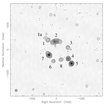
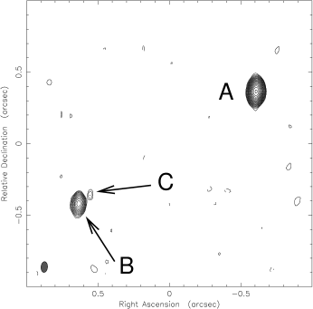
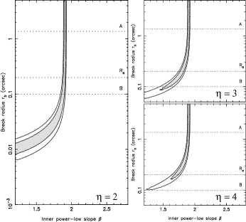
Fig. 3 illustrates a simple gravitational lens with two images located at radii $R_{A}>R_{B}$ from the center of the lens galaxy. Usually we assume a mass distribution $M(<R)$ which produces a ray deflection $\alpha(R)=b\hat{\alpha}(R)\propto M(<R)/R$ consisting of an unknown normalization $b$ multiplied by a deflection profile determined by the mass distribution $\hat{\alpha}(R)$. Because both images must correspond to a common source, the lens equation sets the constraint that

$$-R_{B}+b\hat{\alpha}(R_{B})=R_{A}-b\hat{\alpha}(R_{A})$$ (1)

which is easily solved to find a normalization of

$$b={R_{A}+R_{B}\over\hat{\alpha}(R_{A})+\hat{\alpha}(R_{B})}.$$ (2)

Since the enclosed mass at any radius scales as $b\hat{\alpha}(R)$, you get an accurate estimate for the enclosed mass independent of the profile. In particular, if you use the mass inside the mean image radius, $\langle R\rangle=(R_{A}+R_{B})/2$, then the enclosed mass is independent of the slope ($d\hat{\alpha}/dR$) of the deflection profile and has a fractional dependence on the profile of

$${\Delta M\over M}={1\over 4}\left[{\langle R\rangle^{2}\over\hat{\alpha}}{d^{2}\hat{\alpha}\over dR^{2}}\right]{\Delta R^{2}\over\langle R\rangle^{2}}$$ (3)

that is second order in the asymmetry $\Delta R/\langle R\rangle$ of the image positions. As the lens becomes symmetric, $R_{A}\rightarrow R_{B}$, the images are approaching the Einstein radius and the mass uncertainties diminish rapidly because for any circular lens the mean surface density of the material interior to the Einstein radius $R_{E}$ is exactly $M=\pi R_{E}^{2}\Sigma_{c}$ where $\Sigma_{c}$ is the critical surface density for lensing.

The mass normalization (Eqn. 2) is not very illuminating if our objective is to understand the property of the density distribution constrained by the lensed images. To understand the constraint we start by introducing the mean surface density in an annulus,

$$\langle\kappa_{12}\rangle={2\int_{R_{1}}^{R_{2}}R\kappa(R)dR\over R_{2}^{2}-R_{1}^{2}},$$ (4)

where the mean surface density is related to the mass by $M_{12}=\pi\langle\kappa_{12}\rangle\Sigma_{c}(R_{2}^{2}-R_{1}^{2})$. The ray deflections at the two images are simply

$$b\hat{\alpha}(R_{B})={1\over R_{B}}\langle\kappa_{0B}\rangle R_{B}^{2}\qquad b\hat{\alpha}(R_{A})={1\over R_{A}}\left[\langle\kappa_{0B}\rangle R_{B}^{2}+\langle\kappa_{AB}\rangle(R_{A}^{2}-R_{B}^{2})\right].$$ (5)

Substituting these into the constraint equation (Eqn. 1) we find that

$${1-\langle\kappa_{0B}\rangle\over 1-\langle\kappa_{AB}\rangle}={R_{B}-R_{A}\over R_{B}}<0.$$ (6)

The positions of the two images measure a combination of the mean surface density interior to the inner image and the mean surface density between the two images to the accuracy of the astrometric measurements. This will still hold if we add angular structure to the lens model if we think of the angular deflections as an added source of noise in the constraint. The surface densities are constrained to the range

$$0\leq\langle\kappa_{AB}\rangle\leq 1\leq\langle\kappa_{0B}\rangle\leq\kappa_{max}=R_{A}/R_{B}$$ (7)

with a linear trade off

$$\langle\kappa_{0B}\rangle=\kappa_{max}\left(1-\langle\kappa_{AB}\rangle\right)+\langle\kappa_{AB}\rangle$$ (8)

between the surface densities in which the mass interior to B decreases as we add mass to the annulus between A and B.

The particular combination of surface densities on the left side of Eqn. 6 arises because of the mass sheet degeneracy (Falco et al. [1985]) – given a surface density $\kappa(r)$, the image positions and flux ratios are unchanged if we transform the surface density to by $\kappa(r)\rightarrow(1-\kappa_{0})\kappa(r)+\kappa_{0}$. It is called the mass sheet degeneracy because it corresponds to adding a sheet of surface density $\kappa_{0}$ while reducing the mass scale of the original profile by the factor $1-\kappa_{0}$. Since the right side of Eqn. 6 is a measured quantity, the left side must be invariant under this transformation.

If the lens has additional images in the interior of the annulus, then we can measure more properties of the surface density. The simplest example is to suppose that in addition to the images at $R_{A}$ and $R_{B}$ we also see an Einstein ring image in the annulus at $R_{B}<R_{E}<R_{A}$. As discussed earlier, this is the unique point where the enclosed mass is determined uniquely, with $\langle\kappa_{0E}\rangle=1$ in a spherical lens. The added constraint allows us to determine the ratio

$${1-\langle\kappa_{BE}\rangle\over 1-\langle\kappa_{EA}\rangle}={R_{B}\over R_{A}}{R_{A}^{2}-R_{E}^{2}\over R_{E}^{2}-R_{B}^{2}}>0.$$ (9)

which relates the surface density of the annulus inside the Einstein ring to that outside the Einstein ring. Once again, the constrained quantity combines two mean surface densities in a form which is invariant under the transformation associated with the mass sheet degeneracy.

This brings us to the Gauss’ Laws for (spherical) lens models given a lens with images bounded by the annulus $R_{B}<R<R_{A}$:

• Only the total mass interior to $R_{B}$ and not its distribution is relevant,

• The distribution of mass in the annulus $R_{B}<R<R_{A}$ is relevant only if there are additional lensed images in the annulus, and

• The amount and distribution of mass exterior to $R_{A}$ is irrelevant.

Parametric models must have enough degrees of freedom to vary these quantities, but the constraints on the profile shape apply only in the annulus and only to the extent there are additional constraints. Any extra degrees of freedom in a model beyond the mean annular densities are irrelevant.

If we have a lens like B1933+503 (Sykes et al. [1998]) with 10 lensed images produced by three source components (see Fig. 3), then the density structure in the annulus can be tightly constrained. Fig. 4 shows the constraints obtained by Muñoz et al. ([2001], also see Cohn et al. [2001]) on density distributions of the form $\rho\propto r^{-n}(r^{2}+a^{2})^{1+n/2}$. The acceptable models have parameters ($n\simeq 2$ and $a>>R_{E}$) that lead to nearly flat rotation curves over the annulus bounding the lensed images. Other recent examples are analyses of B0218+357 by Wucknitz et al. ([2004]) and of 0047–2808 by Dye & Warren ([2004]).

Figure 7: The structure of lens galaxies in self-similar models. The top row shows the permitted region for the slope of the inner dark matter cusp ($\rho\propto r^{-n}$) and the projected fraction of the mass $f_{CDM}$ inside $2R_{e}$ composed of dark matter. The results are shown for three ratios $R_{b}/R_{e}$ between the break radius $R_{b}$ of the dark matter profile and the effective radius $R_{e}$ of the luminous galaxy. The solid (dashed) contours show the 68% and 95% confidence levels for two (one) parameter. Note that the estimates of $n$ and $f_{CDM}$ depend little on the location of the break radius relative to the effective radius. The bottom row shows all the mass profiles lying within the (two parameter) 68% confidence region normalized to a fixed projected mass inside $2R_{e}$. For comparison we show the mass enclosed by a de Vaucouleurs model (dotted line) and an SIS (offset dashed line). While the allowed models exhibit a wide range of dark matter abundances, slopes and break radii, they all have roughly isothermal total mass profiles over the radial range spanned by the lensed images.

Another example of an additional constraint is if we can detect a central or odd image at radius $R_{C}<R_{B}$. While there are few examples of central images as yet, their detection will become routine as the sensitivity of radio observations increase. Carrying out the same analysis in terms of mean surface densities that lead to Eqn. 6, we find the constraint

$${1-\langle\kappa_{0C}\rangle\over 1-\langle\kappa_{BC}\rangle}=1+{R_{B}\over R_{C}}$$ (10)

between the mean density $\langle\kappa_{0C}\rangle$ interior to image C and the mean density $\langle\kappa_{BC}\rangle$ between images B and C. If we have a very asymmetric triple in which $\langle\kappa_{0C}\rangle\gg 1$ and $\langle\kappa_{BC}\rangle\gg 1$, then the central density is larger by the factor $1+R_{B}/R_{C}$. The constraint in Eqn. 6 also holds, and it is easy to derive the constraints on other combinations of the mean surface densities to find that they all have the standard form with ratios of $1-\langle\kappa\rangle$ equal to an astrometric constraint. The cleanest present example of a lens with a third image is the radio lens PMNJ1632–0033 (Winn et al. [2002], Winn, Rusin & Kochanek [2004]) shown in Fig. 6. Like B1933+503, the mass distribution is constrained the mass profile is required to be close to isothermal with $1.89<n<1.93$ (see Fig. 6). Routine detection of these central images also offers a new probe for black holes at the centers of the lens galaxy (Mao et al. [2001]) – in the case of PMNJ1632–0033 most models with a black hole as massive as expected from local scalings will produce a fourth image (D) close to image C but about 10 times fainter.

Unfortunately, lenses with additional constraints are relatively rare, so we must find alternate means of breaking the degeneracy. Einstein ring images of the host galaxy can be found relatively easily, but they are better suited for constraining the angular structure of the lens than the radial structure. For lenses without additional constraints this can be done statistically provided the lenses have relatively homogeneous mass distributions. For individual lenses without additional constraints we must either measure the mass $\langle\kappa_{OB}\rangle$ in the interior or measure the surface density of the annulus $\langle\kappa_{AB}\rangle$. The lens constraint Eqn. 6 then supplies the other surface density and we have an absolute measurement of the profile for $R<R_{A}$. A very different approach is to break the degeneracy by using microlensing variability to determine the ratio $\kappa_{*}/\kappa$ between the surface density in stars and the total surface density in the annulus.

3 Statistical Constraints on the Mass Distribution

Analyzing ensembles of lenses to estimate the mean mass distribution has two advantages over analyzing individual lenses. First, it provides constraints over a broad range of radii (relative to $R_{e}$), and second, it breaks the mass sheet degeneracy. The disadvantage of the method is that we must assume the density distributions of lenses are self-similar or at least heterogeneous in a manner that can be included as part of the model. The mass sheet degeneracy is broken because all lenses must agree on the same (scaled) physical density distribution but have source and lens redshifts corresponding to different critical densities. Thus, adding a constant physical density sheet corresponds to adding a different critical density sheet to each lens which cannot be reconciled with the constraints. This approach has been used by Rusin et al. ([2003], [2004]) to estimate both the average mass distribution and the evolution of stellar populations.

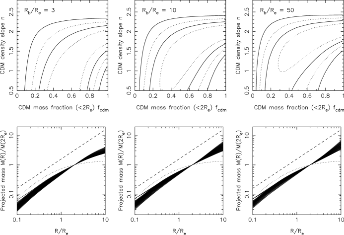
Rusin et al. ([2004]) model the lens galaxy as the sum of a Hernquist model normalized by the observed effective radius of the lens galaxy embedded in a dark matter halo of the form

$$\rho={\rho_{c}\over(r/r_{b})^{n}\left[1+(r/r_{b})^{2}\right]^{(3-n)/2}}$$ (11)

were $r_{b}$ is the break radius and $n$ is the logarithmic slope of the central density cusp. Here we are interested in the dark matter slope $n$ and the fraction of the projected mass inside $2R_{e}$ which is dark matter, although the full calculation includes variables for the scaling of galaxy mass-to-light ratios with redshift and mass. Fig. 7 shows the resulting constraints on the CDM mass fraction projected inside $2R_{e}$ and the logarithmic slope of the central density cusp of the dark matter. While there is a degeneracy in the exact trade-off between the dark matter fraction and the slope, the total mass distribution is well-constrained and close to isothermal (flat rotation curve). The residuals about this mean mass profile can be entirely explained by a realistic spread in the mean stellar ages of the lens galaxies.

Figure 8: Constraints from lens velocity dispersion measurements on the self-similar mass distributions of Fig. 7. The dotted contours show the 68% and 95% confidence limits from the self-similar models for $R_{b}/R_{e}=50$. The shaded regions show the models allowed (68% confidence) by the formal velocity dispersion measurement errors, and the heavy solid lines show contours of the velocity dispersion in km/s. We used the low Gebhardt et al. ([2003]) velocity dispersion for HST14176+5226 because it has the smallest formal error. These models assumed isotropic orbits, thereby underestimating the full uncertainties in the stellar dynamical models.

4 The Stellar Dynamics of Lens Galaxies

If we can use another technique to measure either $\langle\kappa_{AB}\rangle$ or $\langle\kappa_{0B}\rangle$, then we can immediately use the basic lens constraint (Eqn. 6) to determine the other mean surface density and obtain a tight constraint on the density distribution. For example, measuring the stellar velocity dispersion of the lens galaxy will constrain the mass well inside the Einstein radius where it is dominated by stars, roughly corresponding to measuring $\langle\kappa_{0B}\rangle$.

Another way to think about a dynamical measurement is to imagine that the galaxy has a mass profile $M(R)=M_{E}(R/R_{E})^{3-n}$ where we know the mass $M_{E}$ inside the Einstein radius $R_{E}$ accurately from the astrometry of the lensed images but cannot constrain the density exponent $n$. A velocity dispersion measurement corresponds to measuring a virial mass $M_{v}=c_{v}\sigma^{2}R_{v}/G$ on the scale $R_{v}$ of the aperture with a dimensionless constant $c_{v}$ compensating for projection effects, asphericity and orbital anisotropies. Solving for the exponent we find that

$$n=3-\left[\ln(M_{v}/M_{E})\right]\left[\ln(R_{v}/R_{E})\right]^{-1}$$ (12)

and we should be able to determine $n$ to an accuracy of $\delta n\sim(1-2)(\delta\sigma/\sigma)$ since the ratio of the radii is $|\ln(R_{v}/R_{E})|\simeq 1-2$.

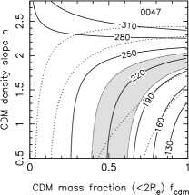
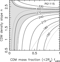
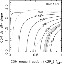
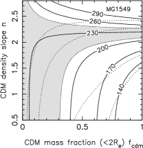
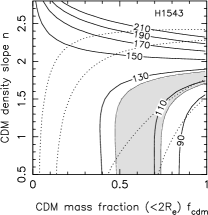
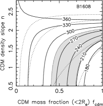
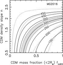
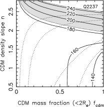
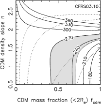
This has been done for 10 systems as illustrated in Fig. 8 using the same parameter space as used for the self-similar models in Fig. 7. With the exception of Q2237+0305, where we see the images in the bulge of a nearby spiral galaxy, the parameter space and degeneracies of the individual velocity dispersion measurements are very similar to the results from the statistical analysis or the models of individual lenses with extra constraints. There are a few lenses which may require more centrally concentrated mass distributions and a falling rotation curve (e.g. PG1115+080), and a few lenses which may require a less centrally concentrated mass distribution and a rising rotation curve (e.g. HST14176+5226). Treu & Koopmans ([2004]) summarize their individual estimates of the mean logarithmic slope of the density finding results scattered about slightly rising rotation curve $\langle n\rangle\simeq 1.9$ with an appreciable rms scatter of $0.30$. The error estimates for the effective slope $n$ seem to be 2–4 times smaller than expected from our simple scaling argument in Eqn. 12. The finding that the typical lens has a rising rotation curve is surprising given the expected halo structure shown in Fig. 1, where we would expect to see a slowly falling rotation curve for $R\mathrel{\raise 1.29167pt\hbox{$>$}\mkern-14.0mu\lower 2.58334pt\hbox{$\sim$}}R_{e}/2$ independent of the baryon fraction.

From Fig. 8 we might naively conclude that the stellar dynamical approach is superior to the statistical approach. However, in producing this comparison, Rusin et al. ([2004]) assumed a simple isotropic dynamical model and the formal uncertainties, which leads to two problems. The first problem is that dynamical measurement uncertainties tend to be underestimated – for example, the three velocity dispersion measurements for HST14176+5226 can be mutually consistent only if their error bars are expanded by 30%. The second problem is that several systematic uncertainties have yet to be included in the comparison. These arise because the distribution of stellar velocities is not Gaussian and because galaxies are not spheres, leading to systematic problems when we use the spherical Jeans equations to analyze the data. The systematics are different from local stellar dynamical estimates because the profile slope (e.g. Eqn. 12) compares a dynamical mass to a lensing mass rather than comparing two dynamical masses. This makes estimates for the mass distribution using the stellar dynamics of lenses sensitive to simple calibration errors $\langle v_{los}^{2}\rangle^{1/2}=f\sigma_{m}$ with $f\neq 1$ between the measurement $\sigma_{m}$ and the rms velocity $\langle v_{los}^{2}\rangle^{1/2}$ in the Jeans equations. Such errors cancel (to lowest order) in a purely stellar dynamical estimate of the mass distribution.

Two simple examples are the effects of non-Gaussian line-of-sight velocity distributions (LOSVDs) and deviations from spherical symmetry. While the Jeans equations depend on $\langle v_{los}^{2}\rangle^{1/2}$, the measurement is usually the dispersion of the best-fit Gaussian, and these two quantities differ by $\langle v_{los}^{2}\rangle^{1/2}\simeq\sigma(1+\sqrt{6}h_{4})$ where $|h_{4}|\mathrel{\raise 1.29167pt\hbox{$<$}\mkern-14.0mu\lower 2.58334pt\hbox{$\sim$}}0.03$ is the dimensionless coefficient of an expansion of the LOSVD in Gauss-Hermite polynomials (e.g. van der Marel & Franx [1993]). The resulting corrections, $|f-1|\simeq\sqrt{6}h_{4}\simeq 7\%$, can be comparable to the formal measurement errors. For example, Romanowsky & Kochanek ([1999]) were able to find models of PG1115+080 consistent with a flat rotation curve where Treu & Koopmans ([2002a]), who used only the Jeans equations, could not. Arguably the distribution functions required to produce the agreement were unusual, but unusual is a very different statement from impossible. Similarly, galaxies are not spheres. From the virial theorem it is easy to show that an oblate ellipsoid of axis ratio $q$ has a ratio between the major and minor axis velocity dispersions that corresponds to a correction of order $|f-1|\simeq(1-q^{2})/5\simeq 16\%$ for $q=0.7$. Making HST14176+5226 a $q=0.7$ galaxy viewed pole on leads to corrections large enough to make this system consistent with a nearly flat rather than a rising rotation curve, thereby eliminating the apparent disagreement between this lens and the results of the statistical analysis. Future analyses of lens dispersions need to treat these systematic uncertainties more carefully since for many purposes they are already larger than the formal measurement errors.

5 Time Delay Measurements

The Party line these days is that the Hubble constant is a known quantity based either on local estimates ($H_{0}=72\pm 8$ km/s/Mpc, Freedman et al. [2001]) or models of CMB fluctuations assuming a flat universe with a cosmological constant ($H_{0}=72\pm 5$ km/s/Mpc, Spergel et al. [2003]). For the purposes of this review, let us assume that the Party is correct and consider its implications. Gravitational lens time delays measure a combination of the Hubble constant and the surface density $\langle\kappa_{AB}\rangle$ in the annulus between the images for which the delay was measured, so if we know $H_{0}$ then time delays provide a very simple means of breaking the degeneracy in Eqn. 6. As in §2, we will discuss only the effects of the radial density distribution. – the effects of the angular distribution are well understood and are reviewed in Kochanek ([2004b]).

The key to understanding time delays comes from Gorenstein et al. ([1988], Kochanek [2002b], see also Saha [2000]) who showed that the time delay in a circular lens depends only on the image positions and the surface density $\kappa(R)$ in the annulus between the images (Fig. 3). A useful approximation is to assume that the surface density in the annulus can be locally approximated by a power law, $\kappa(R)\propto R^{1-n}$ for $R_{B}<R<R_{A}$, with a mean surface density in the annulus of $\langle\kappa_{AB}\rangle$. The time delay between the images is then (Kochanek [2002b])

$$\Delta t=2\Delta t_{SIS}\left[1-\langle\kappa_{AB}\rangle-{1-n\langle\kappa_{AB}\rangle\over 12}\left({\Delta R\over\langle R\rangle}\right)^{2}+O\left(\left({\Delta R\over\langle R\rangle}\right)^{4}\right)\right]$$ (13)

where

$$\Delta t_{SIS}={1\over 2}{D_{OL}D_{OS}\over cD_{LS}}\left(R_{A}^{2}-R_{B}^{2}\right)\propto H_{0}^{-1}$$ (14)

is the time delay for a singular isothermal sphere with comoving angular diameter distances $D_{OL}$, $D_{OS}$ and $D_{LS}$ between the observer, lens and source. The key point is that the time delay is largely determined by the average surface density $\langle\kappa_{AB}\rangle$ in the annulus with only modest corrections from the local shape of the surface density distribution even when $\Delta R/\langle R\rangle\sim 1$. The second order expansion is exact for a singular isothermal lens ($\langle\kappa_{AB}\rangle=1/2$, $n=2$), and it reproduces the time delay of a point mass lens ($\langle\kappa_{AB}\rangle=0$) to better than 1% even when $\Delta R/\langle R\rangle=1$.

Figure 9: $H_{0}$ estimates for PG1115+080. The lens galaxy is modeled as an ellipsoidal pseudo-Jaffe model, $\rho\propto r^{-2}(r^{2}+a^{2})^{-1}$, and the nearby group is modeled as an SIS. As the break radius $a\rightarrow\infty$ the pseudo-Jaffe model becomes an SIS model, and as the break radius $a\rightarrow 0$ it becomes a point mass. The heavy solid curve ($h_{exact}$) shows the dependence of $H_{0}$ on the break radius for the exact, nonlinear fits of the model to the PG1115+080 data. The heavy dashed curve ($h_{scaling}$) is the value found using our simple theory of time delays based on the surface density. The agreement of the exact and scaling solutions is typical. The light solid line shows the average surface density $\langle\kappa\rangle$ in the annulus between the images, and the light dashed line shows the inverse of the logarithmic slope $\eta$ in the annulus ($\kappa\propto R^{1-\eta}$). For an SIS model we would have $\langle\kappa\rangle=1/2$ and $\eta^{-1}=1/2$, as shown by the horizontal line. When the break radius is large compared to the Einstein radius (indicated by the vertical line), the surface density is slightly higher and the slope is slightly shallower than for the SIS model because of the added surface density from the group. As we make the lens galaxy more compact by reducing the break radius, the surface density decreases and the slope becomes steeper, leading to a rise in $H_{0}$. As the galaxy becomes very compact, the surface density near the Einstein ring is dominated by the group rather than the galaxy, so the surface density approaches a constant and the logarithmic slope approaches the value corresponding to a constant density sheet ($\eta=1$).

Figure 10: Our raw light curves for HE0435–1223 (top) and SDSS0924+0219 (bottom). The HE0435–1223 light curve was shifted by 80 days. We have measured the longest time delay in the system (A to D) to 10% accuracy from this data. The B and C images have shorter delays – their different light curve shapes are due to an additional steady fading created by microlensing. In the current season we already see additional intrinsic variability that is increasing the accuracy of the time delay measurements. For SDSS0924+0219 we see little evidence for intrinsic variability – the changes in the flux ratios are entirely due to microlensing. The horizontal lines, referenced to the mean of the A light curve, show the flux ratios when the lens was discovered (HJD–2450000=2259). In the first images of the new season, the fluxes of images A, C and D are little changed, but image B is 0.5 mag fainter. Eventually we expect a dramatic change as image D returns to its expected flux (roughly that of A).

This relationship between annular surface density and time delays is the fundamental relationship to remember. A popular parametric example is the scaling of the time delay for global power law models with $\kappa\propto R^{1-n}$. In these models the mass density scales as $\rho\propto r^{-n}$ and circular velocities or ray deflections scale as $v_{c}^{2}\propto\alpha\propto R^{2-n}$ where $n=2$ is the singular isothermal (SIS) profile producing a flat rotation curve or a constant deflection. In these models the time delay is $\Delta t=\Delta t_{SIS}(n-1)$ to lowest order in $\Delta R/\langle R\rangle$ (Witt et al. [2000]). Although the logarithmic slope $n$ is a global parameter of the model, it enters the time delay only through the general requirements of Eqn. 6 and the surface density of the model near the Einstein ring – the surface density near the Einstein ring is $\langle\kappa_{AB}\rangle=(3-n)/2$, so $1-\langle\kappa_{AB}\rangle=(n-1)$ explains the scaling of the time delay. Fig. 9 shows a more complicated example where we compare estimates of $H_{0}$ from a complex parametric model for PG1115+080 consisting of an ellipsoidal lens plus its parent group to the value we would get simply calculating the surface density of the model and using the generalization of Eqn. 13 for the angular structure of the lens (Kochanek [2002b]). As we would expect from our simple theory, the surface density of the lens and its local slope are all the information needed to predict the scaling of the Hubble constant with the model parameters.

There are presently twelve lenses with published time delay measurements of varying accuracy: B0218+357 (Biggs et al. [1999]), RXJ0911+0551 (Hjorth et al. [2002]), FBQ0951+2635 (Jakobsson et al. [2004]), Q0957+561 (Kundić et al. [1997]), HE1104–1805 (Ofek & Maoz [2003]), PG1115+080 (Schechter et al. [1997]), B1422+231 (Patnaik & Narasimha [2001]), SBS1520+530 (Burud et al. [2002b]), B1600+434 (Burud et al. [2000], Koopmans et al. [2000]), B1608+656 (Fassnacht et al. [2002]), PKS1830–211 (Lovell et al. [1998]) and HE2149–2745 (Burud et al. [2002a]). The interpretation of these delays is controversial (e.g. Williams & Saha [2000], Kochanek [2002b], Koopmans et al. [2003] and references therein), but the problem lies mainly with the limitations of the existing data. The first problem is that several of the lenses are poorly suited to analysis because their photometric structure makes it difficult to perform the accurate astrometry of the images relative to the lens galaxy needed to interpret the delays for any mass distribution. For example, the quasar images are too bright in B0218+357, the lens is too faint in PKS1830–211, and the position estimates depend on accurate corrections for extinction in B1600+434 and B1608+656. The second problem is that many of the delays are not known with sufficient accuracy because the monitoring programs were terminated after the initial delay estimate. We need time delay measurement accuracies of 5% or better in order to have uncertainties in the surface density $\langle\kappa_{AB}\rangle$ that are small compared to the regime of interest ($0.1\mathrel{\raise 1.29167pt\hbox{$<$}\mkern-14.0mu\lower 2.58334pt\hbox{$\sim$}}\langle\kappa_{AB}\rangle\mathrel{\raise 1.29167pt\hbox{$<$}\mkern-14.0mu\lower 2.58334pt\hbox{$\sim$}}0.5$, see Fig. 1). Half of the lenses (FBQ0951+2635, HE1104–1805, PG1115+080, B1422+231, PKS1830–211 and HE2149–2745) have unacceptably high delay uncertainties. The third problem is that we have too few systems to adequately understand environmental effects. While Keeton & Zabludoff ([2004]) somewhat exaggerate the importance of environmental effects on the interpretation of time delays (much of the spread in their distributions is due to the uncertainties in the time delay measurement rather than the effects of the group), it is certainly true that environments affect the interpretation because the parent group or cluster of the lens galaxy contributes to $\langle\kappa_{AB}\rangle$. For example, B1608+656 has two interacting lens galaxies inside the Einstein radius and the lens galaxies of RXJ0911+0551 and Q0957+561 are members of relatively massive clusters where the cluster potential is important to interpreting the time delays. In fact, if we assume the two time delay lenses in clusters (Q0957+561 and RXJ0911+0551) have similar halo structures to the other lenses, then in order to obtain the same value of $H_{0}$ as that of the isolated lenses, the clusters must be contributing significantly to the average surface density ($\kappa_{cluster}\sim 0.1$–$0.3$). Thus, by the time the sample is narrowed to isolated, early-type lenses with good astrometry, good photometry and accurate time delays, almost nothing is left.

As a result, I find much of the recent debate in lensing circles about time delay lenses to be sterile. That one person’s “Golden Lens” can match the Party’s value of $H_{0}$ with a flat rotation curve is largely meaningless when someone else’s “Golden Lens” requires a constant mass-to-light ratio to do so unless you can also provide a coherent explanation of why the mass distributions of the two lenses should be different. Hence the philosophy we adopt here – the Party says $H_{0}$ is known and should not be challenged unless you want to count trees in Siberia, so we should focus on why we cannot produce a coherent story about the structure of lens galaxies at the Party’s value of $H_{0}$ before deciding to attempt a revolution. One possibility, that many delay measurements are less accurate than believed, is easily solved by monitoring the lenses longer. The other possibility, that the halo structures of early-type galaxies are heterogeneous rather than homogeneous, can be addressed independent of the actual value of $H_{0}$.

We can make some initial observations about the homogeneity of halos. If we take the four relatively isolated bulge-dominated time delay lenses (PG1115+080, SBS1520+530, B1600+434 and HE2149–2745), then we can show that for the same value of $H_{0}=100h$km s^-1 Mpc^-1, the lenses must have similar mass distributions. For $H_{0}\simeq 50$km s^-1 Mpc^-1 they can have flat rotation curves, while for $H_{0}\simeq 72$km s^-1 Mpc^-1 their mass distributions must be nearly constant $M/L$ (Kochanek [2002a]). While we cannot (without knowing $H_{0}$) use the time delays to determine which mass distribution is correct, we know that their mass distributions are homogeneous. If we use our surface density formalism, they have mean surface densities of

$$\langle\kappa_{AB}\rangle=1.14-1.21h\pm 0.04,$$

with an upper limit of $\sigma_{\kappa}<0.07$ on the intrinsic scatter in $\langle\kappa_{AB}\rangle$ between the halos. The uncertainties are dominated by the time delay measurement uncertainties for the lenses (Kochanek [2002b]). This result is somewhat puzzling when we compare it to the stellar dynamical results. Treu & Koopmans ([2002a]) argue that PG1115+080 must have a falling rotation curve while the typical lens they have studied has a slightly rising rotation curve (Treu & Koopmans [2004]). But the homogeneity of the surface density estimates based on the time delays indicates that if PG1115+080 has a falling rotation curve then SBS1520+530, B1600+434 and HE2149–2745 must as well. It is odd that the typical time delay lens would have a falling rotation curve while the typical stellar dynamical lens would have a rising rotation curve – the most likely solution is a systematic bias in one of the methods. This will be easily addressed once we have a larger overlapping sample of galaxies with time delay and velocity dispersion measurements.

Figure 11: (LEFT) Dark matter in HE0435–1223. We fit the constraints, including the time delay, starting with a constant $M/L$ de Vaucouleurs model for the stars and then adding an NFW halo (similar to Fig. 1). Here we show the goodness of fit statistic $\chi^{2}$ as a function of the mass of the de Vaucouleurs model relative to its mass in the constant $M/L$ model. The best fit is that the mass of the stellar component can be only $(39\pm 6)\%$ that of a constant $M/L$ model. In this regime, the overall mass distribution has a rotation curve that is very close to flat. At the minimum we have a good fit to the constraints including the geometry of the Einstein ring of the quasar host galaxy.

Figure 12: (RIGHT) An HST image of SDSS0924+0219 stretched to show the flux ratios of the quasar images A–D. In the absence of microlensing (or substructure), the flux of image D should be almost equal to that of image A. Instead, it is an order of magnitude fainter. If this flux ratio anomaly is due to microlensing, we should see it return to its normal flux with quite dramatic color changes for probing the structure of the accretion disk.

Figure 13: (LEFT) The stellar mass fraction $\kappa_{*}/\kappa$ in Q2237+0305. The dashed curve shows the effect of restricting the microlens mass range to $0.2h^{2}M_{\odot}<\langle M\rangle<2h^{2}M_{\odot}$. This eliminates solutions with high effective velocities, so higher stellar densities are needed to produce the same level of variability. We see the Q2237+0305 images through the bulge of a nearby spiral galaxy, so we expect $\kappa_{*}/\kappa\simeq 1$ for this lens.

Figure 14: (RIGHT) Microlensing rates for the first season. The points show fits to the first $dm/dt$ and second $d^{2}m/dt^{2}$ derivatives of the delay-corrected differential light curves for the lensed images in our monitoring sample with adequate data in mid-2004. The point-type changes depending on whether the derivative measurements are consistent with zero. The solid line shows the relation expected for a point source crossing a fold caustic, and the dashed line shows the lower limit on $d^{2}m/dt^{2}$ for a point mass lens. The second derivatives are not very reliable at present because many of the light curves used for the estimates were quite short (months) – we do not see multi-magnitude variations in any of our light curves.

At this point I believe the only good solution is to simply measure many more delays with significantly higher accuracies. With 25 accurate ($<5\%$) time delays in systems with good ancillary data (photometry, astrometry), it will be relatively simple to determine the heterogeneity or homogeneity of early-type galaxy halos. The delay sample will also better overlap systems with extra constraints or stellar dynamical measurements. For a fixed value of $H_{0}$, time delay measurements are a significantly better probe of the halo structure than either statistical studies or stellar velocity dispersion measurements because they are both more accurate and directly measure the quantity of greatest interest, the surface density in the transition region from luminous to dark matter, $\langle\kappa_{AB}\rangle$. We have started such a program using the SMARTS 1.3m telescope in the South and an array of telescopes in the North (MDM, FLWO, APO $\cdots$) to monitor roughly 25 lenses 1-2 times/week when they are visible. Since starting in early 2004 we have measured two new time delays in HE0435–1223 and SDSS1004+4112. We also see an abundance of microlensing variability, whose utility we discuss in §6. Fig. 10 shows the light curves for HE0435–1223 and SDSS0924+0129 from the first season of monitoring.

Fig. 12 shows the results of fitting a model consisting of the luminous lens galaxy and an NFW dark matter halo to HE0435–1223 constrained by the time delay measurement with the Hubble constant fixed to $H_{0}=72$km s^-1 Mpc^-1. If we start from a constant $M/L$ model and then reduce the mass of the luminous galaxy while adding the NFW halo, we see the goodness of fit improves with a minimum where the luminous galaxy has only $(39\pm 6)\%$ of its mass in the constant $M/L$ model. As we improve the delay from its current 10% accuracy, these uncertainties will shrink more or less proportionately.

The other obvious result from our first season is that microlensing of lensed quasars is ubiquitous. In Fig. 10 you can see that the light curves of images A and D in HE0435–1223 are nearly identical while those for B and C look different. Images A and D have the longest delay and are the pair for which we have a time delay measurement. In the first season images B and C were both fading by $0.18\pm 0.02$ mag/year relative to A and D due to microlensing. Other light curves, like the ones for SDSS0924+0129 shown in Fig. 10, show only brightness variations due to microlensing. Collecting and analyzing the microlensing variability is important because it provides our final probe of halo structure using lenses.

6 Microlensing

Microlensing variability depends on both the surface density in stars $\kappa_{*}$ and the total surface density $\kappa$. The regime for a standard halo model is that the total surface density is still relatively high ($\kappa\sim 0.5$) but the stars make up a small fraction of the total ($\kappa_{*}/\kappa\sim 0.1$, see Fig. 1). In this regime, microlensing (or substructure for that matter) has a distinctive statistical pattern that strongly distinguishes between images that are saddle points and minima (Schechter & Wambsganss [2002]). In particular, there is considerable phase space for significantly demagnifying saddle point images. The most dramatic example of this is the (saddle point) image D of SDSS0924+0219, which is almost ten times fainter than expected (see Fig. 12). We can already see in the SDSS0924+0219 light curves of Fig. 10 that the images are being microlensed, but if the suppression of image D is due to microlensing we should eventually see it brighten dramatically, overshooting the flux of image A.

Because the statistical properties of the microlensing patterns depend on $\kappa$ and $\kappa_{*}/\kappa$ we can constrain them by analyzing the light curves. In Kochanek ([2004a]) we developed a method for analyzing microlensing light curves and applied it to the only (hitherto) well-monitored lens Q2237+0305, focusing on the OGLE light curves of Wozniak et al. ([2000]). In this system we see four images of a quasar buried in the bulge of a low redshift spiral galaxy so we would expect to find that $\kappa\simeq\kappa_{*}$, and this is borne out when we analyze the microlensing variability as shown in Fig. 14. Even after including all the other uncertainties (sources sizes, relative velocities $\cdots$) we find that $\kappa_{*}/\kappa>0.5$ if we include no prior assumption on the mean stellar masses, and $\kappa_{*}/\kappa>0.7$ if we force the mean stellar mass to be in the range of $0.1$-$1.0M_{\odot}$.

We do not yet have long enough light curves to make a similar analysis of any other lens, but we are beginning to get there. Fig. 14 shows a crude view of the amount of microlensing, where we estimate the first and second derivatives of the light curves due to microlensing from the data available in mid-2004. Most images have measurable first and second derivatives that cannot be attributed to intrinsic variability. Since we want accurate time delays rather than simply quitting once the delay is measured to 10%, we will be monitoring systems like HE0435–1223 for many more years. The same longer time baselines are needed to obtain useful constraints on the statistical properties of the magnification pattern produced by the stars. The microlensing variability can also be used to probe the structure of quasar accretion disks. For example, even the limited data for SDSS0924+0219 is sufficient to show that it must have an accretion disk that is significantly smaller than that in Q2237+0305, as we might expect from the lower luminosity of SDSS0924+0219.

7 Conclusions

The overall summary of this review is that the future is bright, but the present is painful. On the positive side, we understand the physics of constraining mass distributions with lenses very well. In general, analyses based on image constraints, statistics, velocity dispersions, time delays and microlensing are all generally consistent and indicate that early-type galaxies have appreciable dark matter on intermediate scales ($r\sim 2R_{e}$) leading to a net mass distribution that is close to isothermal for the typical lens. On the negative side, we have not communicated our understanding of how gravitational lenses constrain mass distributions very well. Arguments about methods (parametric versus non-parametric, statistics versus time delays versus dispersions and so on) tend to obscure rather than illuminate the underlying unity of the results.

The fundamental question at this point is the degree to which early-type galaxy halos are heterogeneous in their structures on these scales. Most of this is driven by a fairly familiar astronomical problem. First, there is a preferred, average, naive, straw man, or whatever mass model in which early-type galaxies follow the conspiracy of late-type galaxies and have nearly flat rotation curves with the contribution from the dark matter kicking in just as the contribution from the luminous matter fades. Theoretical halos with the expected baryonic mass fraction would be expected to lie close to this model, usually with a slowly falling rather than a truly flat rotation curve. Second, when we apply the available methods to the lens sample, we find that this is just about right, but there are signs that there is appreciable scatter about the mean. Because of small sample sizes, measurement errors and systematic errors we cannot yet be sure whether this scatter is real and the halo structure is genuinely heterogeneous or if we have simply underestimated our measurement uncertainties. This puts the field in a confused state where everyone argues for their object or method but cannot produce a synthesis of all the available results to produce a convincing final answer. Until we can achieve this synthesis we will continue to have a problem.

Fortunately the way out is straightforward – more data. No one has found a fundamental flaw in any of the methods. The problem is simply that the samples are too small and insufficiently overlapping to produce a clear result. My own feeling is that the method with the least systematic problems for addressing the homogeneity or heterogeneity of early-type galaxy halos is monitoring lenses to measure accurate time delays and comparing the structure of lens galaxies at a fixed value of $H_{0}$. For fixed $H_{0}$, time delays measure the surface density of the galaxy near the lensed images essentially to the accuracy of the time delay measurement, and the surface density near the lensed images is exactly the quantity needed to understand the halo structure. Moreover, the long term monitoring needed to measure accurate time delays also provides microlensing variability light curves that can be used to constrain the fraction of the surface density in the form of stars. There is a very convenient coincidence that the part of parameter space that should be occupied by the lens galaxies in a standard CDM model also has unique microlensing characteristics.