Exploiting the neutronization burst of a galactic supernova

Abstract

One of the robust features found in simulations of core-collapse supernovae (SNe) is the prompt neutronization burst, i.e. the first $\sim 25$ milliseconds after bounce when the SN emits with very high luminosity mainly $\nu_{e}$ neutrinos. We examine the dependence of this burst on variations in the input of current SN models and find that recent improvements of the electron capture rates as well as uncertainties in the nuclear equation of state or a variation of the progenitor mass have only little effect on the signature of the neutronization peak in a megaton water Cherenkov detector for different neutrino mixing schemes. We show that exploiting the time-structure of the neutronization peak allows one to identify the case of a normal mass hierarchy and large 13-mixing angle $\vartheta_{13}$, where the peak is absent. The robustness of the predicted total event number in the neutronization burst makes a measurement of the distance to the SN feasible with a precision of about 5%, even in the likely case that the SN is optically obscured.

I Introduction

Despite the enormous progress of neutrino physics in the last decade, many open questions remain to be solved. Among them are two, the mass hierarchy—normal versus inverted mass spectrum—and the value of the 13-mixing angle $\vartheta_{13}$, where the observation of neutrinos from a core-collapse supernova (SN) could provide important clues Dighe:1999bi ; Lunardini:2003eh ; Takahashi:2003bj . The neutrino emission by a SN can be divided schematically into four stages: Infall phase, neutronization burst, accretion phase, and Kelvin-Helmholtz cooling phase. The bulk of SN neutrinos are emitted in all flavors during the last two phases with small differences between the $\bar{\nu}_{e}$ and $\bar{\nu}_{\mu,\tau}$ spectra Raffelt2001 ; Buras2003 ; Keil2003 . Moreover, the absolute values of the average neutrino energies as well as the relative size of the luminosities during the accretion and cooling phases are not known with sufficient precision. As a consequence, a straightforward extraction of oscillation parameters from the SN neutrino signal during the accretion and cooling phase seems hopeless.

An alternative is the use of observables that do not rely on SN parameters. Such observables require only that the initial neutrino fluxes $F_{i}^{0}$ are different functions of energy and time, $F^{0}_{\nu_{e},\bar{\nu}_{e}}(E,t)\neq F_{\nu_{x},\bar{\nu}_{x}}^{0}(E,t)$, where $x=\{\mu,~{}\tau\}$. Since the interaction of neutrinos with matter depends on their flavor, identical energies and luminosities for $\nu_{e}$, $\bar{\nu}_{e}$ and $\nu_{x}$ would require a conspiracy of interaction rates and chemical composition inside the neutrinospheres. Examples for such observables are the modulations in the SN neutrino signal caused by the passage of the neutrinos through the Earth earth or by the propagation of shock waves through the SN envelope shock ; Tomas:2004gr . If the mixing angle $\vartheta_{13}$ is known to be large, $\sin^{2}\vartheta_{13}\mathrel{\mathop{\kern 0.0pt\hbox to0.0pt{\raise 0.86108pt\hbox{$>$}\hss}}\lower 3.87495pt\hbox{\kern-1.90002pt$\sim$}}10^{-3}$, an observation of Earth matter or shock wave effects in the experimentally most important $\bar{\nu}_{e}$ channel would imply a normal or inverted mass hierarchy, respectively. If however the value of $\vartheta_{13}$ is not known, a degeneracy exists between the case of a normal mass hierarchy and large $\vartheta_{13}$ (scenario A, cf. table 1) and the case of small $\vartheta_{13}$, $\sin^{2}\vartheta_{13}\mathrel{\mathop{\kern 0.0pt\hbox to0.0pt{\raise 0.86108pt\hbox{$<$}\hss}}\lower 3.87495pt\hbox{\kern-1.90002pt$\sim$}}10^{-5}$, and any hierarchy (scenario C): scenario A and C both predict the same $\bar{\nu}_{e}$ signature in a water Cherenkov detector.

A different way to extract reliable information about neutrino mixing parameters is to use characteristics in the neutrino emission of SNe that are model independent. One of the most robust features of numerical SN simulations is the so-called neutronization $\nu_{e}$ burst burst , which takes place during the first $\sim 25$ ms after the core bounce. The small number of events expected during this time period is compensated by the moderate dependence of the $\nu_{e}$ burst on physical parameters like the progenitor mass or details of the SN models. In Sec. II, we discuss the astrophysical aspects of this burst in detail, emphasizing the robustness of the neutrino luminosities against variations in the input of the SN models. In Sec. III, we study the signature of the neutronization peak in a megaton water Cherenkov detector for different neutrino mixing schemes. We argue that exploiting the time-structure of the neutronization peak allows one to identify the neutronization burst even if the SN is not visible in the optical. A non-observation of the neutronization burst identifies the case of a normal mass hierarchy and large 13-mixing angle $\vartheta_{13}$ (case A), thus breaking the degeneracy between the neutrino mixing scenarios A and C. Moreover we find that for a given neutrino mixing scenario the systematic uncertainty due to unknown SN parameters affects only little the total number of events in the neutronization burst. As we discuss in Sec. IV, this robustness of the theoretical prediction makes a measurement of the distance to a SN located at 10 kpc feasible with a precision of about 5%. Such an accuracy is comparable to optical methods using the SN light curve, which have an error between 5 and 10%. If the SN is optically obscured, measuring its distance through the $\nu_{e}$ burst is crucial for estimating the total binding energy released or to limit the strength of the gravitational wave signal Mueller:2003fs emitted by the SN. Finally, we summarize our results in Sec. V.

II Astrophysical aspects of the neutronization burst

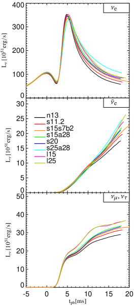
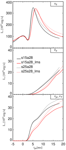
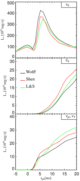
Figure 1: Luminosities as functions of time for $\nu_{e}$ (top), $\bar{\nu}_{e}$ (middle) and heavy-lepton neutrinos (bottom). In the left column results for different progenitor stars between 11.2$\,M_{\odot}$ and 25$\,M_{\odot}$ (left column; the progenitor mass is indicated by the number after the first letter of the model name progenitors ) are shown, in the middle column for simulations with the new treatment of electron captures by nuclei during stellar core collapse according to Langanke, Martínez-Pinedo and Sampaio (LMS; red solid and dotted lines) compared to the traditional description (black lines) in case of a 15$\,M_{\odot}$ and a 25$\,M_{\odot}$ star. The right column shows results for three different nuclear equations of state applied to the collapse of a 15$\,M_{\odot}$ progenitor (see text for more details). The luminosities are given for an observer at rest, evaluated at a radius of 400 km with a corresponding time retardation of about 1 ms. Time is normalized to the moment of shock formation defined by the instant when the entropy behind the shock first exceeds a value of 3 $k_{B}$ per nucleon.

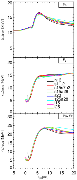
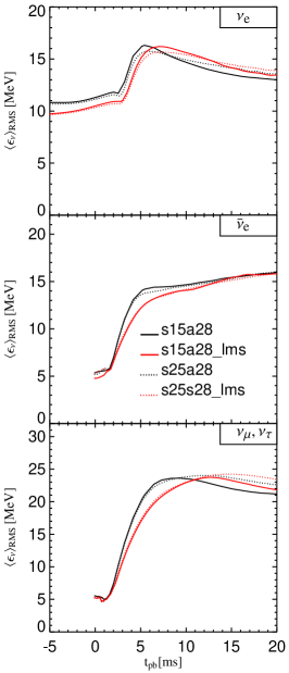
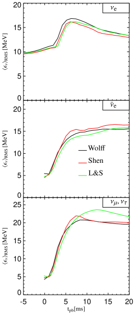
Figure 2: Same as Fig. 1 but for the rms neutrino energies as defined in Eq. (1). Note that during core collapse and in particular before shock formation only $\nu_{e}$ were taken into account in the simulations because the production of $\bar{\nu}_{e}$ and heavy-lepton neutrinos is suppressed due to the low entropy and correspondingly high electron and $\nu_{e}$ degeneracy.

Modern supernova models with sufficiently detailed treatment of the neutrino physics have in common the existence of a “prompt burst” of electron neutrinos promptburst ; Thompson:2002mw ; Liebendoerfer:2002ny . This breakout pulse is launched at the moment when the newly formed supernova shock that races down the density gradient in the collapsing stellar core reaches densities low enough for the initially trapped neutrinos to begin streaming faster than the shock propagates Bethe:1980gq . In the shock-heated matter, which is still rich of electrons and completely disintegrated into free neutrons and protons, a large number of $\nu_{e}$ are rapidly produced by electron captures on protons. They follow the shock on its way out until they are released in a very luminous flash, the breakout burst, at about the moment when the shock penetrates the “neutrinosphere” and the neutrinos can escape essentially unhindered. As a consequence, the lepton number in the layer around the neutrinosphere decreases strongly and the matter neutronizes burrows_mazurek . Because of the high temperatures behind the shock, electron-positron annihilation, nucleon-nucleon bremsstrahlung Thompson:2002mw , and, when $\bar{\nu}_{e}$ become more abundant, also neutrino-pair conversion $\nu_{e}\bar{\nu}_{e}\longrightarrow\nu_{\mu,\tau}\bar{\nu}_{\mu,\tau}$ Buras2003 are efficient in creating muon and tau neutrino-antineutrino pairs . The luminosities of the latter therefore begin rising steeply immediately after shock formation. In contrast, the luminosity of $\bar{\nu}_{e}$ increases more slowly. On the one hand this is due to the fact that the abundance of positrons and therefore the $\bar{\nu}_{e}$ production by $e^{+}$ captures is rather low as long as electrons are still highly degenerate, on the other hand pair creation of $\nu_{e}$ and $\bar{\nu}_{e}$ is also suppressed by the high abundance of $\nu_{e}$ during the burst phase and the corresponding fermion blocking in the $\nu_{e}$ phase space.

These facts can be verified from Figs. 1 and 2. The rms energies shown in the latter figure are defined by

$$\left\langle\epsilon_{\nu}\right\rangle_{\mathrm{RMS}}\,\equiv\,\sqrt{\int_{0}^{\infty}{\mathrm{d}}\epsilon\int_{-1}^{+1}{\mathrm{d}}\mu\,f_{\nu}(\epsilon,\mu)\epsilon^{5}\over\int_{0}^{\infty}{\mathrm{d}}\epsilon\int_{-1}^{+1}{\mathrm{d}}\mu\,f_{\nu}(\epsilon,\mu)\epsilon^{3}}\ ,$$ (1)

with $f_{\nu}(\epsilon,\mu)$ being the neutrino phase space distribution, which is a function of the neutrino energy $\epsilon$ and the cosine, $\mu$, of the angle of neutrino propagation relative to the radial direction. The results presented in the plots were obtained by core collapse simulations in spherical symmetry with the neutrino-hydrodynamics code developed by Rampp and Janka Rampp:2002bq , employing a solver for the energy-dependent moments equations of neutrino number, energy, and momentum and an approximative treatment of general relativity that yields good agreement with fully relativistic simulations, in particular during the collapse and early postbounce phases Liebendoerfer:2003es .

A local minimum in the $\nu_{e}$ luminosities occurs shortly after the formation of the shock at core bounce ($t=0$) and before the neutronization burst. It is caused by the shock first compressing matter from a semi-transparent state to neutrino-opaque conditions before the postshock layer reexpands to become neutrino transparent and to release the neutronization neutrinos Liebendoerfer:2002ny . Performing simulations for a variety of progenitor stars between 11.2$\,M_{\odot}$ and 25$\,M_{\odot}$ from different stellar evolution modelers progenitors , we have confirmed the uniformity of the radiated neutrino luminosities and rms energies in the first 20 ms after bounce (Figs. 1 and 2, left panels) that was also seen in other recent simulations with neutrino transport being described by a solution of the Boltzmann equation or its moments equations Thompson:2002mw ; Liebendoerfer:2002ef . The prompt neutronization burst has a typical full width half maximum of 5–7 ms and a peak luminosity of 3.3–3.5$\times 10^{53}\,$erg s^-1. The striking similarity of the neutrino emission characteristics despite of some variability in the properties of the pre-collapse cores is caused by a regulation mechanism between electron number fraction and target abundances (protons and nuclei) for electron captures Bruenn:1985en ; messerthesis , which establishes similar electron fractions in the inner core during collapse. This leads to a convergence of the structure of the central part (of roughly a solar mass) of the collapsing cores and only small differences in the evolution of different progenitors until shock breakout Liebendoerfer:2002ef . Differences of the core size and of the density profile in the outer part of the iron core and beyond lead to different mass infall rates at late times when the shock has reached neutrino-transparent layers. This implies different accretion luminosities and thus causes a progenitor-dependent strong variation of the neutrino emission characteristics after the $\nu_{e}$ luminosity has levelled off from the prompt burst.

Only recently improvements in the treatment of electron capture rates on nuclei during the late phases of stellar evolution and core collapse have become available which remove shortcomings of the widely used independent particle model in which electron captures are suppressed by Pauli blocking for nuclei with $N\geq 40$ Bruenn:1985en . This typically happens at a density of some $10^{10}\,$g cm^-3 above which electron captures on free protons govern the evolution of the electron fraction. The improved rates for core collapse are based on Shell Model Monte Carlo calculations of nuclear properties at finite temperatures, complemented with a Random Phase Approximation for the electron capture rates of a wide sample of nuclei in the mass range between $A=65$ and $A=112$ with abundances given by nuclear statistical equilibrium Langanke:2003ii . In supernova simulations with these improved rates electron captures by nuclei dominate over capture on free protons, and interesting changes were found during core collapse, bounce, and postbounce evolution Langanke:2003ii ; Hix:2003fg . In the panels of the middle columns of Figs. 1 and 2 one can see the corresponding differences in the neutrino emission properties for simulations of a 15$\,M_{\odot}$ and a 25$\,M_{\odot}$ progenitor with the new capture rates according to Langanke, Martínez-Pinedo and Sampaio (LMS) Langanke:2001td in comparison to runs with the traditional rate treatment. Despite of the visible variations with the rate treatment, however, the spread of results for different progenitors does not widen and again the core properties seem to converge during collapse by a self-regulation of electron captures. It is unlikely that this result will change when incoherent neutrino scattering off nuclei is included in the models. The effects of this process during stellar core collapse have not been satisfactorily explored yet.

There is still considerable uncertainty in the supernova simulations due to our incomplete knowledge of the nuclear equation of state. The runs for the different progenitors as well as the studies with varied electron capture rates were all performed with the nuclear equation of state (EoS) of Lattimer and Swesty (L&S) lsmodel , which is most widely used in core collapse simulations. It is based on a compressible liquid drop model and employs a Skyrme force for the nucleon interaction. Our choice of the compressibility modulus of bulk nuclear matter was 180 MeV, and the symmetry energy parameter 29.3 MeV, but the differences in the supernova evolution caused by other values of the compressibility of this EoS were shown to be minor Thompson:2002mw ; swestymira .

We have recently tested the effects of the nuclear EoS by using two available alternative descriptions marekdiploma ; Janka:2004tt , on the one hand a new relativistic mean field EoS (“Shen”) shenmodel with a compressibility of nuclear matter of 281 MeV and a symmetry energy of 36.9 MeV, and on the other hand an EoS which was constructed by Hartree-Fock calculations with a Skyrme force for the nucleon-nucleon interaction (“Wolff”) wolffmodel and has a compressibility of 263 MeV and a symmetry energy of 32.9 MeV. In particular the latter EoS allows for a faster deleptonization of the less compact and less opaque postshock layer, thus producing a clearly higher $\nu_{e}$ burst in comparison to the standard case with L&S EoS. Note that all three runs were performed with the 15$\,M_{\odot}$ progenitor model s15a28 of Woosley et al. progenitors and included the use of the new LMS rates for electron captures.

Uncertainties of core collapse simulations due to the use of different numerical schemes for hydrodynamics and neutrino transport were recently investigated in a comparison of the Oak Ridge-Basel and Garching supernova codes Liebendoerfer:2003es . Despite of differences in details, very satisfactory agreement was found for the overall evolution and for the neutrino emission properties. The approximative description of general relativity in the Garching code produces only insignificant deviations from the fully relativistic treatment of the Oak Ridge-Basel code during the infall phase and early postbounce evolution including the prompt neutronization burst. The burst heights and widths agree nicely between both codes in Newtonian as well as relativistic runs.

Among the remaining systematic uncertainties in core collapse models with possible consequences for the neutronization burst is the unsettled question of rotation in the progenitor core. While the large asymmetries seen in supernova explosions are sometimes claimed to be caused by rapid core rotation (e.g., Ref. Burrows:2004va ), recent stellar evolution models seem to disfavor this possibility because they predict that massive stars lose angular momentum very efficiently during their evolution. The stellar cores therefore rotate so slowly — rotation periods at the edge of the iron core before the onset of gravitational instability were determined to be around 100 s — that core collapse and bounce remain essentially unaffected by rotational effects Heger:2004qp . Instead of rotation, low-mode convective instabilities have been discussed in this case as potential origin of the observed global anisotropies of supernovae Blondin:2002sm ; Scheck:2003rw . For a more reliable determination of the conditions in the pre-collapse cores, however, truely multi-dimensional stellar evolution models are desired instead of the currently used spherical ones that are supplemented by evolution equations for the lateral averages of the angular momentum and magnetic field.

If rapid rotation of the pre-collapse iron is still considered as a viable possibility, despite of probably valid objections based on current stellar evolution models, one may wonder about the effects of such rotation on the prompt $\nu_{e}$ burst. For having a noticeable influence, the central spin period before collapse must be significantly less than 3–5 s, which decreases during collapse by a factor of about 100. Unfortunately, all numerical studies of rotational core collapse published so far were done with very simplistic or no treatment of neutrino transport (see, e.g., Ref. kotake and references therein), and only the paper by Fryer and Heger Fryer:1999he provides information in some detail about the neutrino emission, although the grey diffusion scheme used in that work falls much behind the quality and refinement of the transport discussed here for simulations of nonrotating (or sufficiently slowly rotating) collapsing stars. Besides a possible dependence of the neutrino signal from the viewing angle (as a consequence of the rotational deformation of the core and differences of the shock propagation and breakout between pole and equator moenchmeyer ), the magnitude of the neutronization burst and the mean energies of neutrinos emitted during the burst seem to be reduced by rapid rotation Fryer:1999he . For conclusive results, however, one has to await simulations with a better treatment of neutrino transport.

III Analysis of the neutrino signal

III.1 Neutrino fluxes

The neutrino flux spectra $F_{\nu_{i}}$ arriving at the Earth are determined by the primary neutrino fluxes $F^{0}_{\nu_{i}}$ as well as the neutrino mixing scenario,

$$F_{\nu_{e}} = pF_{\nu_{e}}^{0}+(1-p)F_{\nu_{x}}^{0}\,,$$ (2)

$$F_{\bar{\nu}_{e}} = \bar{p}F_{\bar{\nu}_{e}}^{0}+(1-\bar{p})F_{\nu_{x}}^{0}~{},$$ (3)

$$4F_{\nu_{x}} = (1-p)F_{\nu_{e}}^{0}+(1-\bar{p})F_{\bar{\nu}_{e}}^{0}+(2+p+\bar{p})F_{\nu_{x}}^{0}\,,\quad$$ (4)

where $p$ $(\bar{p})$ is the survival probability of an electron (anti-)neutrino after propagation through the SN mantle and the interstellar medium. We restrict our analysis to the standard case of three active neutrino flavors and negligible magnetic moments or decays . We assume also that the neutrinos do not cross the Earth before reaching the detector. The main consequence of Earth matter effects on $\nu_{e}$ neutrinos—the key channel to observe the neutronization burst—is a regeneration effect in scenario B and C, thereby slightly improving the chances to detect the $\nu_{e}$ burst, while Earth matter effects have no impact on the signal in scenario A. Therefore, Earth matter effects increase the differences between scenario A and B/C and it is conservative to neglect them in our analysis.

The probabilities $p$ and $\bar{p}$ are basically determined by the flavor conversions that take place in the resonance layers, where $\rho_{\rm res}\approx m_{\rm N}\Delta m^{2}_{i}\cos 2\vartheta/(2\sqrt{2}G_{\rm F}Y_{\rm e}E)$. Here $\Delta m^{2}_{i}$ and $\vartheta$ are the relevant mass difference and mixing angle of the neutrinos, $m_{\rm N}$ is the nucleon mass, $G_{\rm F}$ the Fermi constant and $Y_{\rm e}$ the electron fraction. In contrast to the solar case, SN neutrinos must pass through two resonance layers: the H-resonance layer at $\rho_{\rm H}\sim 10^{3}$ g/cm³ corresponds to $\Delta m^{2}_{\rm atm}$, whereas the L-resonance layer at $\rho_{\rm L}\sim 10$ g/cm³ corresponds to $\Delta m^{2}_{\odot}$ . This hierarchy of the resonance densities, along with their relatively small widths, allows the transitions in the two resonance layers to be considered independently Dighe:1999bi .

The neutrino survival probabilities can be characterized by the degree of adiabaticity of the resonances traversed, which are directly connected to the neutrino mixing scheme. In particular, the L-resonance is always adiabatic and appears only in the neutrino channel, whereas the adiabaticity of the H-resonance depends on the value of $\vartheta_{13}$, and the resonance appears in the neutrino or anti-neutrino channel for a normal or inverted mass hierarchy, respectively. Table 1 shows the survival probabilities for electron neutrinos, $p$, and anti-neutrinos, $\bar{p}$, in various mixing scenarios for the static density profile of the progenitor. Using this profile is appropriate, because we are only interested in the neutrino propagation during the first milliseconds after core-bounce when the shock wave has not reached the H-resonance yet Tomas:2004gr . For intermediate values of $\vartheta_{13}$, i.e. $10^{-5}\mathrel{\mathop{\kern 0.0pt\hbox to0.0pt{\raise 0.86108pt\hbox{$<$}\hss}}\lower 3.87495pt\hbox{\kern-1.90002pt$\sim$}}\sin^{2}\vartheta_{13}\mathrel{\mathop{\kern 0.0pt\hbox to0.0pt{\raise 0.86108pt\hbox{$<$}\hss}}\lower 3.87495pt\hbox{\kern-1.90002pt$\sim$}}10^{-3}$, the survival probabilities are no longer constant but depend on the neutrino energy as well as on the details of the density profile of the SN.

Scenario	Hierarchy	$\sin^{2}\vartheta_{13}$	$p$	$\bar{p}$
A	Normal	$\mathrel{\mathop{\kern 0.0pt\hbox to0.0pt{\raise 0.86108pt\hbox{$>$}\hss}}\lower 3.87495pt\hbox{\kern-1.90002pt$\sim$}}10^{-3}$	0	$\cos^{2}\vartheta_{\odot}$
B	Inverted	$\mathrel{\mathop{\kern 0.0pt\hbox to0.0pt{\raise 0.86108pt\hbox{$>$}\hss}}\lower 3.87495pt\hbox{\kern-1.90002pt$\sim$}}10^{-3}$	$\sin^{2}\vartheta_{\odot}$	0
C	Any	$\mathrel{\mathop{\kern 0.0pt\hbox to0.0pt{\raise 0.86108pt\hbox{$<$}\hss}}\lower 3.87495pt\hbox{\kern-1.90002pt$\sim$}}10^{-5}$	$\sin^{2}\vartheta_{\odot}$	$\cos^{2}\vartheta_{\odot}$

Table 1: Survival probabilities for neutrinos, $p$, and anti-neutrinos, $\bar{p}$, for various mixing scenarios in case of the density profile of the SN progenitor. Terms of the order $\vartheta_{13}^{2}$ and smaller have been neglected. The solar mixing angle is assumed to be $\sin^{2}\vartheta_{\odot}=0.30$; for a recent discussion of allowed neutrino oscillation parameters see Ref. Maltoni:2004ei .

For large values of $\vartheta_{13}$, $\sin^{2}\vartheta_{13}\mathrel{\mathop{\kern 0.0pt\hbox to0.0pt{\raise 0.86108pt\hbox{$>$}\hss}}\lower 3.87495pt\hbox{\kern-1.90002pt$\sim$}}10^{-3}$, the H-resonance is adiabatic. In the case of a normal mass hierarchy, scenario A, the resonance takes place in the neutrino channel. Then practically all $\nu_{e}$ which are initially created as $\nu_{3}$ leave the SN also as $\nu_{3}$. When they reach the detector, they have only a small $\nu_{e}$ admixture, $\langle\nu_{3}|\nu_{e}\rangle=\sin\vartheta_{13}$. Taking into account the experimental constraints on $\vartheta_{13}$, $\sin^{2}\vartheta_{13}\mathrel{\mathop{\kern 0.0pt\hbox to0.0pt{\raise 0.86108pt\hbox{$<$}\hss}}\lower 3.87495pt\hbox{\kern-1.90002pt$\sim$}}0.047$ at $3\sigma$ C.L. Maltoni:2004ei , one obtains $p^{\rm A}=\sin^{2}\vartheta_{13}\mathrel{\mathop{\kern 0.0pt\hbox to0.0pt{\raise 0.86108pt\hbox{$<$}\hss}}\lower 3.87495pt\hbox{\kern-1.90002pt$\sim$}}0.047$. This corresponds to an almost complete interchange of the $\nu_{e}$ and $\nu_{x}$ spectra. For an inverted mass hierarchy, scenario B, the resonance occurs in the anti-neutrino channel, thus interchanging now almost completely the $\bar{\nu}_{e}$ and $\bar{\nu}_{x}$ spectra. In contrast, the H-resonance is strongly non-adiabatic for small values of $\vartheta_{13}$, $\sin^{2}\vartheta_{13}\mathrel{\mathop{\kern 0.0pt\hbox to0.0pt{\raise 0.86108pt\hbox{$<$}\hss}}\lower 3.87495pt\hbox{\kern-1.90002pt$\sim$}}10^{-5}$, and for any mass hierarchy (scenario C), and hence it is ineffective. In both the scenarios B and C, the primary $\nu_{e}$ leave the star as $\nu_{2}$ with a large $\nu_{e}$ admixture at the detector, $\langle\nu_{2}|\nu_{e}\rangle=\sin\vartheta_{\odot}$, leading to $p^{\rm B,C}=\sin^{2}\vartheta_{\odot}=0.30$ Maltoni:2004ei .

Let us assume for simplicity that during the neutronization bursts only $\nu_{e}$ neutrinos are emitted. Then the neutrino fluxes arriving at the Earth are in scenario A

$$F^{\rm A}_{\nu_{e}} = p^{\rm A}F_{\nu_{e}}^{0}+(1-p^{\rm A})F_{\nu_{x}}^{0}\approx 0\,,$$ (5)

$$2F^{\rm A}_{\nu_{x}} = (1-p^{\rm A})F_{\nu_{e}}^{0}+(1+p^{\rm A})F_{\nu_{x}}^{0}\approx F_{\nu_{e}}^{0}\,,$$ (6)

and in scenario B or C,

$$F^{\rm B,C}_{\nu_{e}} = p^{\rm B,C}F_{\nu_{e}}^{0}+(1-p^{\rm B,C})F_{\nu_{x}}^{0}\approx\sin^{2}\vartheta_{\odot}F_{\nu_{e}}^{0}\,,\quad$$ (8)

$$2F^{\rm B,C}_{\nu_{x}} = (1-p^{\rm B,C})F_{\nu_{e}}^{0}+(1+p^{\rm B,C})F_{\nu_{x}}^{0}$$ (9)

$$\approx \cos^{2}\vartheta_{\odot}F_{\nu_{e}}^{0}\,.\quad$$

Hence a detector able to identify $\nu_{e}$ events will observe a peak in the $\nu_{e}$ channel in the cases B and C, while the peak would be completely absent in case A. The signature is similar, although less dramatic, for a detector observing elastic scattering events. In this case not only $\nu_{e}$ but also $\nu_{x}$ contribute to the signal through neutral-current reactions. But since the cross section for elastic scattering on electrons is larger for $\nu_{e}$ than for $\nu_{x}$ neutrinos, the event number during the neutronization burst even for such a non-ideal detector is much larger in the scenarios B and C than in A.

Finally, we note from Fig. 1 that the emission of other flavors than $\nu_{e}$ becomes important already during the end of the neutronization burst, washing out the big differences expected in the naive picture above. In the next subsection, we discuss in detail how the neutronization burst can be identified.

III.2 Detection of the neutronization burst

Theoretically, the identification of the neutronization burst is cleanest with a detector using the charged-current absorption of $\nu_{e}$ neutrinos. Examples of such detectors are heavy water detectors like SNO sno using $\nu_{e}+d\to e^{-}+p+p$, or liquid argon detectors like ICARUS Gil-Botella:2003sz using $\nu_{e}+{}^{40}{\rm Ar}\to e^{-}+{}^{40}{\rm K}^{\ast}$.

The simplest possible observable to identify the neutronization burst is the total number $N$ of $\nu_{e}$ events within an arbitrary fixed period $t_{\max}$ after the onset of the neutrino signal. For instance, Ref. Gil-Botella:2003sz calculated the expected number of $\nu_{e}+{}^{40}{\rm Ar}\to e^{-}+{}^{40}{\rm K}^{\ast}$ events in a 70-kton liquid argon detector for $t_{\max}=240$ ms, where $t=200$ ms corresponds to the core bounce, assuming one specific astrophysical model and as SN distance $d=10$ kpc. They found $N=41$ events in scenario A, compared to $N=86$ in scenarios B and C. From the discussion in Sec. II, it is clear that the uncertainty in $N$ coming from SN models is rather small. We will quantify this uncertainty later in Sec. III.3.2 and use here 10% as estimate for the systematic uncertainties due to the SN models. Combining these systematic uncertainties and the statistical fluctuations in quadrature leads to $N=41\pm 8$ for scenario A and $N=86\pm 13$ for B and C. Thus one could conclude that a differentiation between the scenarios A and B/C on the 2 $\sigma$ level is possible with a liquid argon detector using the total number of events. However, we have still neglected another important source of uncertainty for $N$: The distance to stars in our Galaxy is typically known only with 25% accuracy distanceaccuracy . The measurement of the SN lightcurve will allow a determination of its distance with an error of $\approx 5$–10% pm . However, the probability that the SN is obscured by dust is as high as $\sim$75%. Without an estimate for the SN distance, the total number of events observed cannot be connected to the SN luminosity and is thus not a useful observable. Instead, we exploit in the following the time structure of the detected neutrino signal as signature for the neutronization burst.

Since the $\nu_{e}$ burst lasts only about 25 ms, cf. Fig. 1, the event number in current and proposed charged-current detectors is not high enough to allow for a detailed time analysis. Therefore, we will concentrate in the following on the case of a megaton water Cherenkov detector, proposed e.g. to be build in Japan HK or in the United States uno . A drawback of this choice is that this detector type does not have a clean signature for the $\nu_{e}$ channel. Instead, one has to consider the $\nu_{e}$ elastic scattering on electrons, $\nu_{e}+e^{-}\rightarrow\nu_{e}+e^{-}$. This reaction is basically affected by three different kinds of backgrounds: inverse beta decay reactions $\bar{\nu}_{e}+p\rightarrow n+e^{+}$, reactions on oxygen, and the elastic scattering of other neutrino flavors on electrons. In Fig. 3, we show the distribution of the reconstructed energies and directions with respect to the vector SN-Earth made of all events in a water Cherenkov detector for $t<t_{\max}=18$ ms, where $t_{\rm bounce}=0$ ms. The events are simulated following Ref. Tomas:2003xn .

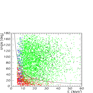
Figure 3: Energy and angular distribution of all events with $t<t_{\max}=18$ ms, assuming $t_{\rm bounce}=0$ ms at bounce, in a megaton water Cherenkov detector for a SN with a progenitor mass of $15~{}M_{\odot}$ at 5 kpc, and scenario C. The different reaction channels shown are elastic scattering on electrons (red), inverse beta decay (green), CC events on oxygen (black) and NC events on oxygen (blue); also shown is the cut $E({\rm MeV})\times{\rm angle}({\rm degrees})=500$.

The dominant source of background events are inverse beta decay reactions. These events are almost isotropically distributed, while their energy distribution reflects the neutrino energy spectrum. In contrast, elastic scattering events are concentrated in the forward direction and at rather low energies. Therefore a cut with $E({\rm MeV})\times{\rm angle(deg)}<500$ as shown in Fig. 3 by a solid black line substantially reduces the number of background events while keeping most of elastic scattering events. This background is further reduced by using in addition Gadolinium to tag the neutrons produced in the inverse beta reaction Beacom:2003nk . Reactions on oxygen have a large reaction threshold, $E_{\rm th}>15$ MeV, and are therefore not numerous. Moreover, the charged-current events on oxygen (black dots) have an angular distribution peaked slightly backwards, and thus the chosen cut eliminates these events efficiently, too.

As illustration for the efficiency of the background suppression we show in Fig. 4 the expected signal without (solid lines) and with cuts (dashed lines). In both cases we assumed an efficiency of 90% for the Gd tagging of the inverse beta decay reactions. While the number of elastic scattering events is practically unchanged, the background of inverse beta decays and reactions on oxygen is significantly reduced. Therefore, we will consider only the elastic scattering reactions on electrons in our discussion below. The sample of elastic scattering events still contains the irreducible background of scattering on electrons of other neutrinos than $\nu_{e}$, but we will show that it is possible to disentangle the scenarios with and without peak even in the presence of this background.

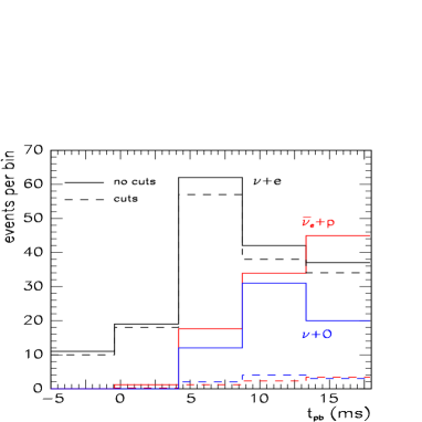
Figure 4: Number of events per time bin from the elastic scattering on electrons (black), inverse beta decay assuming 90% tagging efficiency of Gadolinium (red), and reactions on oxygen (blue) in a megaton water Cherenkov detector for a SN with a progenitor mass of $15~{}M_{\odot}$ at 10 kpc, and case C. Solid lines stand for the number of events without cut and dashed lines with the cut $(E/{\rm MeV})\times({\rm angle}/{\rm degrees})=500$.

III.3 Results

In this subsection, we examine in detail how the prompt neutronization burst from a future galactic SN appears in a water Cherenkov detector. For this purpose, we have generated elastic scattering events of neutrinos on electrons using Monte Carlo simulations as described in Ref. Tomas:2003xn . If not otherwise stated, we have assumed a megaton detector with energy threshold $E_{\rm th}=5$ MeV and 10 kpc as the distance to the SN. If the energy threshold could be lowered to 3 MeV, then the event number would typically increase by 20%. The neutrino luminosities and energy spectra are based on the SN models described in Sec. II. In order to follow the time evolution of the signal, we have considered the time interval from $t=-5$ ms until $t=18$ ms postbounce and divided the interval into five bins. As far as the neutrino mixing scenario is concerned, we will compare only the cases A and C. The first reason for this choice is that the differences between B and C arising in the anti-neutrino channel, $\bar{p}^{\rm B}\neq\bar{p}^{\rm C}$, are always smaller than their differences to case A. Secondly, the mixing scenario B can be confirmed or ruled out by the modulations in the $\bar{\nu}_{e}$ spectrum induced by shock waves in the SN envelope or by Earth matter effects, respectively. However, these modulations are not helpful to distinguish the cases A and C, since $\bar{p}^{\rm A}=\bar{p}^{\rm C}$ .

III.3.1 Dependence on the neutrino mixing scenario

To understand better the results of our Monte Carlo simulations, we first discuss qualitatively the behavior of the expected signal in the presence of the irreducible $\nu_{x}$ background. The total number of events can be decomposed as

$$N(t)=N_{\nu_{e}}(t)+N_{\bar{\nu}_{e}}(t)+N_{\nu_{x}}(t)+N_{\bar{\nu}_{x}}(t)\,,$$ (10)

where $N_{\nu_{i}}(t)$ represents the number of events produced in the reaction $\nu_{i}+e^{-}\rightarrow\nu_{i}+e^{-}$. Since we are interested in the differences between scenario A and C, and $\bar{p}^{\rm A}=\bar{p}^{\rm C}$, we will concentrate on the number of events produced by $\nu_{e}e^{-}$ and $\nu_{x}e^{-}$ scatterings. Taking into account the linear dependence of the cross sections on the neutrino energy, $\sigma_{\nu e}(E)\approx\sigma^{0}_{\nu e}E$, and Eqs. (2–4), we can write

$$N_{\nu_{e}}(t) \propto \sigma^{0}_{\nu_{e}e}\left[pL_{\nu_{e}}(t)+(1-p)L_{\nu_{x}}(t)\right]\,,$$ (11)

$$N_{\nu_{x}}(t) \propto \sigma^{0}_{\nu_{x}e}\left[(1-p)L_{\nu_{e}}(t)+(1+p)L_{\nu_{x}}(t)\right]\,,$$ (12)

where $\sigma^{0}_{\nu_{e}e}\approx 6\sigma^{0}_{\nu_{x}e}$. We parameterize our simulation results for the different neutrino luminosities by $L_{\nu_{x}}(t)=\varepsilon(t)L_{\nu_{e}}(t)$, where $\varepsilon(t)$ is zero until core bounce ($t_{\rm pb}=0$ ms), increases afterwards, and reaches $\varepsilon(t)\approx 0.5$ at $t_{\rm pb}=18$ ms.

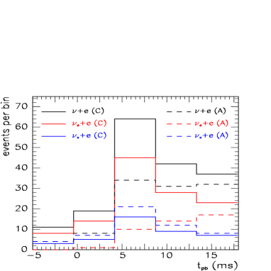
Figure 5: Number of events per time bin from the elastic scattering on electrons: total number (black), $\nu_{e}~{}e$ (red) and $\nu_{x}~{}e$ (blue), for the mixing scenarios C (solid lines) and A (dashed lines). A megaton water Cherenkov and a SN with progenitor mass 15 $M_{\odot}$ at 10 kpc is assumed.

We now examine the difference in the total number of events between scenario A and C. We define the following ratio,

$$R_{\nu}^{\rm AC}(t)\equiv\frac{N^{\rm A}_{\nu_{e}}(t)+N^{\rm A}_{\nu_{x}}(t)}{N^{\rm C}_{\nu_{e}}(t)+N^{\rm C}_{\nu_{x}}(t)}\approx\frac{1+7~{}\varepsilon(t)}{2.5+5.5~{}\varepsilon(t)}\,.$$ (13)

In the first three bins $\varepsilon(t)\approx 0$ and, therefore, all events are generated from $F^{0}_{\nu_{e}}$. In scenario C, 30% of the original $\nu_{e}$ remain as $\nu_{e}$ whereas 70% are converted into $\nu_{x}$. In case A, almost all $\nu_{e}$ arrive at the Earth as $\nu_{x}$. Since the cross section is smaller for $\nu_{x}e^{-}$ than for $\nu_{e}e^{-}$, fewer events are expected in scenario A. This difference, though, is not constant but changes with $\varepsilon(t)$, from $R_{\nu}^{\mathrm{AC}}(t)\approx 0.4$ right before the bounce until 0.9 at $t_{\rm pb}=18$ ms. This evolution can be clearly observed in the behavior of the solid (case C) and dashed (case A) black lines in Fig. 5, showing the most important contributions to the neutronization burst signal, $\nu_{e}e^{-}$ (red) and $\nu_{x}e^{-}$ (blue), and the total $\nu e^{-}$ (black).

Next, we study the different contributions from $\nu_{e}$ and $\nu_{x}$ scatterings to the signal. In particular, from Eqs. (11–12) we define the ratio

$$R_{ex}(t)\equiv\frac{N_{\nu_{e}}(t)}{N_{\nu_{x}}(t)}\approx 6\>\frac{p+(1-p)~{}\varepsilon(t)}{1-p+(1+p)~{}\varepsilon(t)}\,.$$ (14)

In case C, $R^{\rm C}_{ex}(t)>1$ during the whole burst. Therefore, $\nu_{e}e^{-}$ scatterings generate always more events than $\nu_{x}e^{-}$ reactions, as can be seen in Fig. 5. This is very different in case A: The value of the ratio, $R^{\rm A}_{ex}(t)\approx 6\varepsilon(t)/(1+\varepsilon(t))$, strongly depends on time. In the first two bins, $\varepsilon(t)\approx 0$, and thus $R^{\rm A}_{ex}(t)\approx 0$. Therefore, practically all events are generated by $\nu_{x}e^{-}$. At $t_{\rm pb}\mathrel{\mathop{\kern 0.0pt\hbox to0.0pt{\raise 0.86108pt\hbox{$>$}\hss}}\lower 3.87495pt\hbox{\kern-1.90002pt$\sim$}}11$ ms, however, $\varepsilon(t)$ has increased so much that $R^{\rm A}_{ex}\mathrel{\mathop{\kern 0.0pt\hbox to0.0pt{\raise 0.86108pt\hbox{$>$}\hss}}\lower 3.87495pt\hbox{\kern-1.90002pt$\sim$}}1$. In Fig. 5, we can see how in the first three bins the dashed blue lines are above the red ones, but in the fourth bin both lines cross and events from $\nu_{e}e^{-}$ scatterings become more important. This feature will play a key role in disentangling both mixing scenarios.

Finally, we discuss the time evolution of the signal. This evolution results from an interplay of the time dependence of $L_{\nu_{e}}(t)$ and $L_{\nu_{x}}(t)$. Whereas $L_{\nu_{e}}(t)$ shows a clear peak structure around $t_{\rm pb}\approx 7$ ms, $L_{\nu_{x}}(t)$ steadily increases after the bounce. In order to discuss which time behavior dominates, we consider separately the two channels $N_{\nu_{e}}(t)$ and $N_{\nu_{x}}(t)$. From Eqs. (11–12), we can estimate the ratio between events connected to $L_{\nu_{x}}(t)$ and to $L_{\nu_{e}}(t)$. In scenario C, this ratio is smaller than one for both channels $N_{\nu_{e}}(t)$ and $N_{\nu_{x}}(t)$. Thus the component generated by $L_{\nu_{e}}(t)$, and therefore producing a clear peak, dominates over $L_{\nu_{x}}(t)$. This is reflected in Fig. 5 in the peak structure of both the solid red and blue lines. In scenario A, the ratio is smaller than one in $N_{\nu_{x}}(t)$, but it is larger that one in $N_{\nu_{e}}(t)$. Therefore, $L_{\nu_{e}}(t)$ dominates over $L_{\nu_{x}}(t)$, if $R^{\rm A}_{ex}(t)<1$. As a consequence, the net result in scenario C is an enhanced peak, whereas in scenario A the time structure is more complicated. In the first three bins, $N_{\nu_{x}}(t)$ dominates over $N_{\nu_{e}}(t)$ producing a peak like in case C, but with fewer events. In the fourth and fifth bin, however, $N_{\nu_{e}}(t)$ becomes larger and there is a cancellation between the negative slope of $N_{\nu_{x}}(t)$ and the positive of $N_{\nu_{e}}(t)$. The final result is an almost flat structure in case A (dashed black lines in Fig. 5), in contrast to the clear decrease of events in the last two bins in case C.

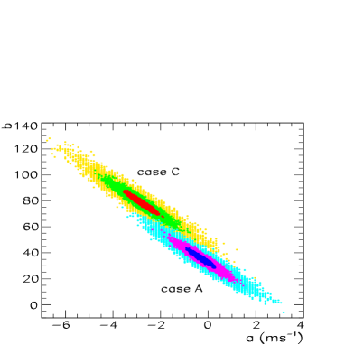
Figure 6: Distribution of fit values $a$ and $b$ for different SN distances, $D=2,5$ and 10 kpc, and a $15~{}M_{\odot}$ SN progenitor.

In order to illustrate the difference in the slope after the third bin we have simulated the neutrino signal from 10000 SN explosions for a progenitor with $15~{}M_{\odot}$. Then we have fitted the last three bins in each case by a straight line, $y=at/{\rm ms}+b$. In Fig. 6, we show the normalized distribution of the fit values of $a$ and $b$ for scenarios A and C and three different distances, $D=2,5$ and 10 kpc. The slope, $a$, is centered at almost 0 ms^-1 in mixing scenario A, whereas in C the center lies at about $-3~{}{\rm ms}^{-1}$.

III.3.2 Dependence on the progenitor mass and SN models

We have discussed how the presence or absence of a peak in the neutrino signal during the neutronization burst is related to the neutrino mixing scenario. In this subsection, we analyze the robustness of this connection, studying its dependence on several SN parameters.

If the SN is optically obscured, then the progenitor cannot be identified. Thus we have to ensure that the neutrino signal during the $\nu_{e}$ burst depends only weakly on the progenitor model. We have analyzed the expected neutrino signal for various progenitors with main sequence masses $11.2~{}M_{\odot}$ (s11.2), $13~{}M_{\odot}$ (n13), $15~{}M_{\odot}$ (s15s7b2), $15~{}M_{\odot}$ (s15a28), $20~{}M_{\odot}$ (s20) and $25~{}M_{\odot}$ (s25a28) progenitors . In Fig. 7, we show for illustration the results for two extreme progenitors, n13 and s25a28, as well as for an intermediate case, s15s7b2.

We find that for all progenitor masses the peak structure described in the last subsection can be clearly observed in case C but not in case A. In the first three bins the differences between different progenitor masses are smaller than the statistical fluctuations. The average event number per bin varies less than 6% changing the progenitor mass from $11~{}M_{\odot}$ to $25~{}M_{\odot}$. This variation is at least a factor two smaller than the statistical fluctuations. However, after the third bin the predictions for different progenitor models vary more strongly, reaching 10% or the size of the statistical fluctuations. At this time, neutrinos other than $\nu_{e}$ start to play an important role and the predictions become more model-dependent, cf. Fig. 1. These differences, though, do not affect the observation of the neutronization peak, and therefore do not spoil the possibility to disentangle the scenarios A and C.

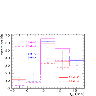
Figure 7: Number of events per time bin for different reactions in a megaton water Cherenkov detector for a SN at 10 kpc for cases A (dashed lines) and C (solid lines) and for different progenitor masses: $13~{}M_{\odot}$ (n13) in red, $15~{}M_{\odot}$ (s15s7b2) in magenta, and $25~{}M_{\odot}$ (s25a28) in blue. Statistical errors are also shown for the $15~{}M_{\odot}$ case.

Another source of uncertainty in our predictions of the neutrino signal may be the incomplete or inaccurate treatment of some of the weak interaction rates, in particular with nuclei, used in the SN simulations. As an example for the changes in the neutrino signal induced by an improved treatment of these rates we consider the effect of electron captures by nuclei in the core. We compare the signal expected for the progenitor models s15a28 and s25a28, see Fig. 8, with and without including the electron capture rates on nuclei with mass numbers larger than 65 as suggested in Ref. Hix:2003fg (LMS). In both s15a28 and s25a28 SN models we observe the main differences in the central bins. This change is directly connected to the behavior of the luminosities: Electron capture on heavy nuclei broadens the peak in $L_{\nu_{e}}(t)$ and reduces somewhat $L_{\nu_{x}}(t)$. However, the changes are always smaller than the statistical fluctuations and therefore do not affect the observation of the neutronization peak.

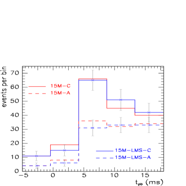
Figure 8: Same as Fig. 7 for mixing scenarios A (dashed lines) and C (solid lines) for a SN at 10 kpc and a progenitor mass of $15~{}M_{\odot}$ (s15a28). In blue we show the SN model with the electron capture rates on heavy nuclei adopted from Ref. Langanke:2003ii (LMS), and in red with the traditional description. Statistical errors are also shown for the (LMS) models.

For the SN progenitor s15a28 we have also investigated the influence of the nuclear equation of state (EoS) on the evolution of the luminosity during the neutronization burst. We have considered three different models for the EoS, dubbed “L&S” lsmodel , “Shen” shenmodel , and “Wolff” wolffmodel . In Fig. 9 we show the predicted numbers of events depending on the employed EoS. The main change is the total luminosity in the peak. In case C, the change in the luminosities results only in a rescaling of the total number of events in each bin. In case A, though, the increase of $L_{\nu_{e}}$ leads to an enhancement of the $\nu_{x}+e^{-}$ contribution, whereas the $\nu_{e}+e^{-}$ events are not strongly affected. As can be seen in Fig. 5, this may slightly modify the time-structure and may lead to a small peak in the third bin. However, these changes are again much smaller than the size of the statistical fluctuations.

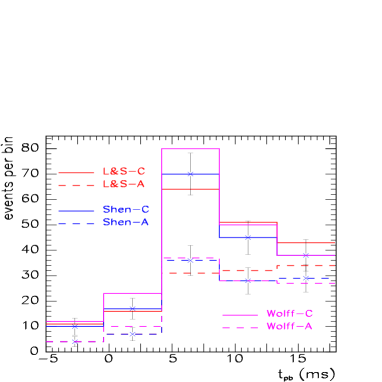
Figure 9: Same as Fig. 7 for mixing scenarios A (dashed lines) and C (solid lines) for a SN at 10 kpc and a progenitor mass of $15~{}M_{\odot}$ (s15a28). We show the SN models computed with the equations of state “L&S” (red), “Shen” (blue), and “Wolff” (magenta), respectively. Statistical errors are displayed for the “Shen” model.

In summary, we have found that the changes in the predicted event numbers for different progenitor models, improvements in the interaction rates or changes in the EoS are small compared to the size of the statistical fluctuations. However, up to now we have always varied only one parameter, e.g. the progenitor mass, and kept all others fixed. In order to quantify the probability to disentangle the neutrino mixing scenarios A and C, we should in principle first quantify the uncertainties in all input parameters of the SN model and then derive the resulting uncertainties in the neutrino fluxes. Already the first step is impractical. Therefore, we use the following method: We take all the SN models considered in the previous sections and calculate for each the expected number of events for cases A, $N_{\alpha,i}^{\rm A}$, and C, $N_{\alpha,i}^{\rm C}$, where $\alpha$ refers to a SN model. Then we compute the probability that scenario A and C can be distinguished for all possible pairs $\alpha,\beta$ using a $\chi^{2}$ analysis,

$$\chi^{2}_{\rm AC}(\alpha,\beta)=\sum_{\rm i=1}^{5}\frac{(N_{\alpha,i}^{\rm A}-N_{\beta,i}^{\rm C})^{2}}{N_{\alpha,i}^{\rm A}+N_{\beta,i}^{\rm C}}\,.$$ (15)

In Fig. 10 we plotted with solid lines the distribution of this probability using all possible combinations of the SN models introduced previously. In the worst combination, scenario A and C can be distinguished only at the $2\sigma$ level ($p=4.5\%$). However, in most cases the probability to misidentify scenarios A and C is smaller than $3\sigma$ ($p=0.27\%$). We show in Fig. 10 also the case that the systematic uncertainty of the SN models is dominated by the unknown progenitor star (dashed line). Then it is possible to disentangle the scenarios A and C with a confidence level better than $3\sigma$ for most combinations.

Figure 10: Distribution of the probability to misidentify cases A and C for all SN models considered in the previous sections combined (solid lines), and only for those with different progenitor mass (dashed lines).

III.3.3 Intermediate values of $\vartheta_{13}$ and scenario B

For completeness, we analyze in this subsection the dependence of the neutrino signal on intermediate values of $\vartheta_{13}$ in scenario A, and the case of scenario B. For this purpose we fix a SN progenitor model, s15a28, and consider first mixing scenarios that lie between A and C, i.e. a normal mass hierarchy and $\sin^{2}\vartheta_{13}=10^{-3}$, $5\times 10^{-5}$, $2\times 10^{-5}$ and $10^{-6}$, see Fig. 11. The first and the last value correspond to scenario A and C, respectively. Whereas $\bar{p}(E)$ is independent on $\vartheta_{13}$, the average value of $p(E)$ grows continuously from 0 in mixing scenario A to $\sin^{2}\vartheta_{\odot}\approx 0.3$ in scenario C. This behavior of the $\nu_{e}$ survival probability results in a continuous increase of the peak. For instance, the probability to disentangle the case of intermediate $\vartheta_{13}$ from scenario A becomes smaller than 2$\sigma$ for $\sin^{2}\vartheta_{13}\mathrel{\mathop{\kern 0.0pt\hbox to0.0pt{\raise 0.86108pt\hbox{$>$}\hss}}\lower 3.87495pt\hbox{\kern-1.90002pt$\sim$}}10^{-5}$ and the SN progenitor s15a28. Therefore, the detection of a peak not only excludes case A ($\sin^{2}\vartheta_{13}\mathrel{\mathop{\kern 0.0pt\hbox to0.0pt{\raise 0.86108pt\hbox{$>$}\hss}}\lower 3.87495pt\hbox{\kern-1.90002pt$\sim$}}10^{-3}$), but also most of the intermediate range of $\vartheta_{13}$, $\sin^{2}\vartheta_{13}\mathrel{\mathop{\kern 0.0pt\hbox to0.0pt{\raise 0.86108pt\hbox{$>$}\hss}}\lower 3.87495pt\hbox{\kern-1.90002pt$\sim$}}10^{-5}$.

Finally, we show also an example of case B, inverted mass hierarchy and large $\vartheta_{13}$, $\sin^{2}\vartheta_{13}=10^{-2}$. Since the survival probability for anti-neutrinos is different for B and C, the total number of events also differs slightly. In particular, the number of events in case B is expected to be larger, as it can be seen in Fig. 11. The reason is twofold: First, $L_{\bar{\nu}_{x}}>L_{\bar{\nu}_{e}}$, and second $\sigma_{\bar{\nu}_{e}e}>\sigma_{\bar{\nu}_{x}e}$. Since $\bar{p}^{\rm B}\approx 0$, more $\bar{\nu}_{x}$ are converted into $\bar{\nu}_{e}$ than in case C, and the larger $\bar{\nu}_{e}~{}e^{-}$ cross section implies more events. Hence, we conclude that scenario B is slightly easier to distinguish from C than A from C.

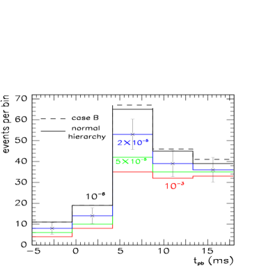
Figure 11: Same as Fig. 7 for a SN at 10 kpc and a progenitor mass of $15~{}M_{\odot}$ (s15a28), for different neutrino parameters. We show with a dashed line case B, inverted mass hierarchy, and with solid lines a normal mass hierarchy for different values of $\sin^{2}\vartheta_{13}$. Statistical errors are shown for $\sin^{2}\vartheta_{13}=2\times 10^{-5}$.

IV Distance determination

After the neutrino mixing scenario has been determined, the small spread in the predicted total number of events $N$ suggests that $N$ is a useful estimator for the SN distance $D$. Since $D\propto N^{1/2}$, the relative uncertainty $\delta N/N_{0}$ translates into

$$\delta D=\frac{D_{0}}{2N_{0}}\delta N\,.$$ (16)

For each SN model $\alpha$, the probability distribution $p_{\alpha}(N)$ of the observed number of events $N$ is Gaussian with $\sigma_{\rm stat}=\sqrt{\langle N_{\alpha}\rangle}$. To estimate the “systematic” uncertainty $\sigma_{\rm syst}$ due to differences in the SN models, we use the following recipe: We calculate for different models the individual expectation value $\langle N_{\alpha}\rangle$ and use then their variance as systematic uncertainty, i.e.

$$\sigma_{\rm sys}^{2}=\frac{1}{m-1}\sum_{\alpha=1}^{m}\left(\langle N_{\alpha}\rangle-\langle N\rangle\right)^{2}\,,$$ (17)

where $m$ stands for the total number of SN models considered, and $\langle N\rangle=(1/m)\sum_{\alpha}\langle N_{\alpha}\rangle$.

The two most important sources of systematic errors are the nuclear equation of state, $\sigma^{\rm EoS}_{\rm sys}$ and, if the SN progenitor is not identified, its mass, $\sigma^{\rm mass}_{\rm sys}$. In order to quantify the influence of different progenitor types we have considered six different SN models (s11.2, n13, s15s7b2, s15a28, s20, and s25a28) discussed in Sec. II. For the time interval considered here, from $t=-5$ ms until $t=18$ ms post bounce, we obtain as systematic error $\sigma^{\rm mass}_{\rm sys}\approx 7$%. In the case of a SN located at 10 kpc we expect as average value $\langle N\rangle=112$ and $\sigma^{\rm mass}_{\rm syst}\approx 8$ as systematic error for scenario A, compared to $\langle N\rangle=176$ and $\sigma^{\rm mass}_{\rm syst}\approx 12$ for scenario C. In Fig. 12, we show the probability distribution $p_{\alpha}(N)$ of the observed number of events $N$ until $t=18$ ms post bounce, choosing as examples three SN models: s15s7b2, and the extreme cases n13 and s25a28. The obtained range $[\langle N\rangle-\sigma^{\rm mass}_{\rm sys}:\langle N\rangle+\sigma^{\rm mass}_{\rm sys}]$ is also shown by arrows for scenarios A and C.

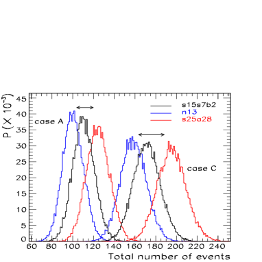
Figure 12: Distribution $p_{\alpha}(N)$ of the observed total number of events $N$ for 20000 simulated SNe with progenitors

: n13, s15s7b2, and s25a28, and for the neutrino mixing scenarios A and C. A distance to the SN of 10 kpc has been assumed.

The second source of systematic uncertainty analyzed is the nuclear equation of state. As an illustration of its effect on the determination of the SN distance we have considered the SN progenitor s15a28 using the three different EoS defined in Sec. II: L&S, Shen and Wolff. While the energy emitted in $\nu_{e}$ and $\nu_{x}$ until $t=18$ ms post bounce in the models L&S and Shen differs by less than 3%, the energy released in the Wolff model differs by more than 16%. This difference depends on the flavor: in the Wolff model more $\nu_{e}$’s but fewer $\nu_{x}$’s are emitted than in the other models. In scenario C the signal is dominated by $L_{\nu_{e}}$, and thus the number of events in the Wolff model is much larger than in the other two models. However, in scenario A the contribution from $L_{\nu_{x}}$ is of the same order of magnitude as that of $L_{\nu_{e}}$, and since $L_{\nu_{x}}$ is smaller in the Wolff model, this compensates the increase in the number of events due to $L_{\nu_{e}}$. This leads to much less variation in the total number of events in case A than in C. For the same time interval we have obtained a systematic error $\sigma^{\rm EoS}_{\rm sys}\approx 2$% and 6% in cases A and C, respectively. If a SN is located at 10 kpc we expect as average value $\langle N\rangle=106$ and $\sigma^{\rm EoS}_{\rm syst}\approx 2$ as systematic error for scenario A, compared to $\langle N\rangle=189$ and $\sigma^{\rm EoS}_{\rm syst}\approx 12$ for scenario C. In Fig. 13, we show the probability distribution $p_{\alpha}(N)$ of the observed number of events $N$ until $t=18$ ms post bounce for the three different models considered. The corresponding range $[\langle N\rangle-\sigma^{\rm EoS}_{\rm sys}:\langle N\rangle+\sigma^{\rm EoS}_{\rm sys}]$ is also shown by arrows for scenario A and C.

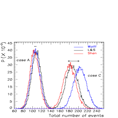
Figure 13: Same as Fig. 12 for the SN progenitor s15a28 and three different EoS: L&S, Shen and Wolff.

Assuming that $\sigma^{\rm mass}_{\rm sys}$ and $\sigma^{\rm EoS}_{\rm sys}$ dominate the total systematic uncertainty $\sigma_{\rm sys}$ we obtain a total “systematic error” of 7% and 9% for scenarios A and C, respectively. We can now combine the statistical errors associated with the averages $\langle N\rangle$ and systematical errors again in quadrature. For the cases discussed in this section this results in a relative error of 12% for the total event number, or a 6% error in the SN distance as predicted from the prompt neutronization burst.

This result represents a significant improvement with respect to the typical accuracy of the distance determination for stars in our Galaxy, which is of the order of 25%. In the case that the SN lightcurve can be measured, the distance to the star could be determined with a similar accuracy, 5–10%. However, it is likely that the next Galactic SN is obscured by interstellar dust: about three out of four SNe are estimated to be optically obscured by dust pm . In this case the measurement of the neutrino signal from the neutronization burst would provide the only way to determine the distance to the star.

V Summary

We have performed simulations of SN explosions for a variety of progenitor models and differences in the underlying microphysics used. The resulting changes in the neutrino signal from the neutronization burst were always small compared to the statistical fluctuations expected for a megaton water Cherenkov detector. We have argued that the total number of events is not a useful observable, if the SN is optically obscured by dust. Instead, we propose to use the time structure of the neutrino signal as discriminator for the neutrino mixing scenario: the observation of a peak in the first milliseconds of the neutrino signal would rule out the normal mass hierarchy with “large” $\vartheta_{13}$ (case A), cf. Figs. 6–9. Thereby, the degeneracy between scenarios A and C, which both produce the same $\bar{\nu}_{e}$ signal during the accretion and cooling phases, can be broken.

After the neutrino mixing scenario has been established, the small uncertainty in the predicted value of the total event rate during the neutronization burst phase makes a determination of the SN distance feasible independent from optical observations. Provided that the predictions of current progenitor models and state-of-the-art simulations do not miss important physics, we estimate that the SN distance can be measured with an accuracy of $\sim$6%. Since it is likely that a Galactic SN is optically obscured by interstellar dust and no other distance determination can be used, this new method relying only on neutrinos seems very promising.

- (1) A. S. Dighe and A. Y. Smirnov, Phys. Rev. D 62, 033007 (2000) [hep-ph/9907423].
- (2) C. Lunardini and A. Y. Smirnov, JCAP 0306 (2003) 009 [hep-ph/0302033].
- (3) K. Takahashi and K. Sato, Nucl. Phys. A 718 (2003) 455.
- (4) G. G. Raffelt, Astrophys. J. 561, 890 (2001) [astro-ph/0105250];
- (5) R. Buras, H.-T. Janka, M. T. Keil, G. G. Raffelt and M. Rampp, Astrophys. J. 587, 320 (2003) [astro-ph/0205006].
- (6) M. T. Keil, G. G. Raffelt and H.-T. Janka, Astrophys. J. 590, 971 (2003) [astro-ph/0208035].
- (7) C. Lunardini and A. Y. Smirnov, Nucl. Phys. B 616, 307 (2001) [hep-ph/0106149]; K. Takahashi and K. Sato, Phys. Rev. D 66, 033006 (2002) [hep-ph/0110105]; A. S. Dighe, M. T. Keil and G. G. Raffelt, JCAP 0306, 006 (2003) [hep-ph/0304150]; A. S. Dighe, M. Kachelrieß, G. G. Raffelt and R. Tomàs, JCAP 0401, 004 (2004) [hep-ph/0311172].
- (8) R. C. Schirato and G. M. Fuller, astro-ph/0205390; G. L. Fogli, E. Lisi, D. Montanino and A. Mirizzi, Phys. Rev. D 68 (2003) 033005 [hep-ph/0304056].
- (9) R. Tomàs, M. Kachelrieß, G. Raffelt, A. Dighe, H.-T. Janka and L. Scheck, JCAP 0409, 015 (2004) [astro-ph/0407132].
- (10) For a review, see A. Burrows, “Neutrinos from Supernovae”, in Supernovae, A. G. Petschek (Ed.), Springer, New York (1990), p. 143.
- (11) E. Müller, M. Rampp, R. Buras, H.-T. Janka and D. H. Shoemaker, “Towards gravitational wave signals from realistic core collapse supernova models,” Astrophys. J. 603, 221 (2004) [astro-ph/0309833].
- (12) S. W. Bruenn, Phys. Rev. Lett. 59, 938 (1987); R. Mayle, J. R. Wilson and D. N. Schramm, Astrophys. J. 318, 288 (1987); E. S. Myra and A. Burrows, Astrophys. J. 364, 222 (1990); M. Rampp and H.-T. Janka, Astrophys. J. 539, L33 (2000) [astro-ph/0005438]; M. Liebendörfer, A. Mezzacappa, F. K. Thielemann, O. E. B. Messer, W. R. Hix and S. W. Bruenn, Phys. Rev. D 63, 103004 (2001) [astro-ph/0006418]; M. Liebendörfer, O. E. B. Messer, A. Mezzacappa, S. W. Bruenn, C. Y. Cardall and F. K. Thielemann, Astrophys. J. Suppl. 150, 263 (2000).
- (13) T. A. Thompson, A. Burrows and P. A. Pinto, Astrophys. J. 592, 434 (2003) [astro-ph/0211194].
- (14) M. Liebendörfer, A. Mezzacappa, O. E. B. Messer, G. Martinez-Pinedo, W. R. Hix and F. K. Thielemann, Nucl. Phys. A 719, 144 (2003) [astro-ph/0211329].
- (15) H. A. Bethe, J. H. Applegate and G. E. Brown, Astrophys. J. 241, 343 (1980).
- (16) A. Burrows and T. J. Mazurek, Astrophys. J. 259, 330 (1982).
- (17) M. Rampp and H.-T. Janka, Astron. Astrophys. 396, 361 (2002) [astro-ph/0203101].
- (18) M. Liebendörfer, M. Rampp, H.-T. Janka and A. Mezzacappa, astro-ph/0310662.
- (19) K. Nomoto and M. Hashimoto, Phys. Rep. 163, 13 (1988) (Model n13); S. E. Woosley and T. A. Weaver, Astrophys. J. Suppl. 101, 181 (1995) (Model s15s7b2); Woosley, S.E., Heger, A., and Weaver, T.A. 2002, Rev. Mod. Phys. 74, 1015 (2002) (Models s11.2, s20, s15a28, s25a28); M. Limongi, O. Straniero, and A. Chieffi, Astrophys. J. Suppl. 129, 625 (2000) (Models l15, l25).
- (20) M. Liebendörfer, O. E. B. Messer, A. Mezzacappa, W. R. Hix, F. K. Thielemann and K. Langanke, “The importance of neutrino opacities for the accretion luminosity in spherically symmetric supernova models,” Procs. 11th Workshop on Nuclear Astrophysics, Ringberg Castle, Tegernsee, Germany, Feb. 11–16, 2002, Wolfgang Hillebrandt and Ewald Müller (Eds.); MPA-Report P13, MPI für Astrophysik, Garching (2002) p. 126 [astro-ph/0203260].
- (21) S. W. Bruenn, Astrophys. J. Suppl. 58, 771 (1985).
- (22) O. E. B. Messer, PhD Thesis, University of Tennessee (2000); Bulletin of the American Astronomical Society, Vol. 33, p.1411 (2001).
- (23) K. Langanke et al., Phys. Rev. Lett. 90, 241102 (2003) [astro-ph/0302459].
- (24) W. R. Hix et al., Phys. Rev. Lett. 91, 201102 (2003) [astro-ph/0310883].
- (25) K. Langanke, G. Martinez-Pinedo and J. M. Sampaio, Phys. Rev. C 64, 055801 (2001) [nucl-th/0101039].
- (26) J. M. Lattimer, C. J. Pethick, D. G. Ravenhall and D. Q. Lamb, Nucl. Phys. A 432, 646 (1985); J. M. Lattimer and F. D. Swesty, Nucl. Phys. A535, 331 (1991).
- (27) F. D. Swesty, J. M. Lattimer, and E. S. Myra, Astrophys. J. 425, 195 (1994).
- (28) A. Marek, Diploma Thesis, Technische Universität München (TUM) 2003.
- (29) H.-T. Janka, R. Buras, F. S. Kitaura Joyanes, A. Marek and M. Rampp, “Core-Collapse Supernovae: Modeling between Pragmatism and Perfectionism,” in: Proceedings of 12th Workshop on Nuclear Astrophysics, Ringberg Castle, Tegernsee, March 22–27, 2004, Eds. E. Müller and H.-Th. Janka, Report MPA-P14, Max-Planck-Institut für Astrophysik, Garching, p. 150 (2004) [astro-ph/0405289].
- (30) H. Shen, H. Toki, K. Oyamatsu and K. Sumiyoshi, Nucl. Phys. A 637, 435 (1998) [nucl-th/9805035]; Prog. Theor. Phys. 100, 1013 (1998) [nucl-th/9806095].
- (31) W. Hillebrandt, R. G. Wolff and K. Nomoto, Astron. Astrophys. 133 175 (1984); W. Hillebrandt and R. G. Wolff, in Nucleosynthesis: Challenges and New Developments, W. D. Arnett and J. W. Truran (Eds.), Univ. Chicago Press (1985), p. 131.
- (32) A. Burrows, R. Walder, C. D. Ott and E. Livne, “Rotating Core Collapse and Bipolar Supernova Explosions,” in The Fate of the Most Massive Stars, Proc. Eta Carinae Science Symposium, Jackson Hole, May 23–28, 2004, ASP Conference Series (2005) [astro-ph/0409035].
- (33) A. Heger, S. E. Woosley and H. C. Spruit, astro-ph/0409422.
- (34) J. M. Blondin, A. Mezzacappa and C. DeMarino, Astrophys. J. 584, 971 (2003) [astro-ph/0210634].
- (35) L. Scheck, T. Plewa, H.-T. Janka, K. Kifonidis and E. Müller, Phys. Rev. Lett. 92, 011103 (2004) [astro-ph/0307352].
- (36) K. Kotake, S. Yamada, and K. Sato, Astrophys. J. 618, 474 (2005).
- (37) C. L. Fryer and A. Heger, Astrophys. J. 541, 1033 (2000).
- (38) H. -T. Janka and R. Mönchmeyer, Astron. Astrophys. 209, L5 (1989); Astron. Astrophys. 226, 69 (1989).
- (39) S. Ando and K. Sato, JCAP 0310, 001 (2003) [hep-ph/0309060].
- (40) E. K. Akhmedov and T. Fukuyama, JCAP 0312 007 (2003) [hep-ph/0310119].
- (41) S. Ando, Phys. Rev. D 70 033004 (2004) [hep-ph/0405200].
- (42) M. Maltoni, T. Schwetz, M. A. Tórtola and J. W. F. Valle, hep-ph/0405172.
- (43) http://www.sno.phy.queensu.ca/
- (44) I. Gil-Botella and A. Rubbia, JCAP 0310, 009 (2003) [hep-ph/0307244].
- (45) H. Scheffler and H. Elsässer, Physics of the Galaxy and Interstellar Matter, Springer-Verlag, Berlin 1988.
- (46) P. Mazzali, private communcation.
- (47) Y. Itow et al., arXiv:hep-ex/0106019.
- (48) The UNO whitepaper, “Physics Potential and Feasibility of UNO,” available at http://ale.physics.sunysb.edu/uno/.
- (49) R. Tomàs, D. Semikoz, G. G. Raffelt, M. Kachelrieß and A. S. Dighe, Phys. Rev. D 68, 093013 (2003) [hep-ph/0307050]. The neutral current events on oxygen have been simulated following E. Kolbe, K. Langanke and P. Vogel, Phys. Rev. D 66, 013007 (2002).
- (50) J. F. Beacom and M. R. Vagins, Phys. Rev. Lett. 93, 171101 (2004) [hep-ph/0309300].