Metallicities on the Double Main Sequence of $\omega$ Centauri
Imply Large Helium Enhancement

Abstract

Having shown in a recent paper that the main sequence of $\omega$ Centauri is split into two distinct branches, we now present spectroscopic results showing that the bluer sequence is less metal-poor. We have carefully combined GIRAFFE@VLT spectra of 17 stars on each side of the split into a single spectrum for each branch, with adequate $S/N$ to show clearly that the stars of the blue main sequence are less metal poor by 0.3 dex than those of the dominant red one. From an analysis of the individual spectra, we could not detect any abundance spread among the blue main sequence stars, while the red main sequence stars show a 0.2 dex spread in metallicity. We use stellar-structure models to show that only greatly enhanced helium can explain the color difference between the two main sequences, and we discuss ways in which this enhancement could have arisen.

1 Introduction

Omega Centauri is the Galactic globular cluster (GC) with the most complex stellar population, and a huge amount of attention has been paid to it. Its high mass may represent a link between GCs and larger stellar systems. Understanding the star-formation history in $\omega$ Cen might give fundamental information on the star-formation processes in more complex systems such as galaxies.

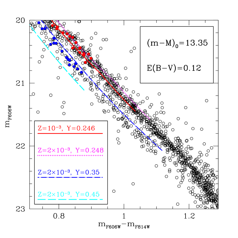
Figure 7: Comparison of the ACS CMD of $\omega$ Cen  (calibrated following Bedin et al. 2004b) with isochrones calculated for the metallicity determined in Fig. 1. The bMS can be reproduced only assuming $Y>0.35$. The blue and red filled dots show the bMS and rMS stars for which we collected our spectra.

The problem is that the more information we acquire on the stars of $\omega$ Cen, the less we understand their origin. In this respect, the most recent and most puzzling result surely is the identification of a double main sequence (DMS)—originally discovered by Anderson (1997), and discussed in detail by Bedin et al. (2004a, B04), who showed that the feature is real, and present throughout the cluster. As far as we know, $\omega$ Cen  is the only GC to show two MS populations. But what makes this result even more enigmatic is the color distribution of the stars on the DMS. If we were to guess what the MS should look like from what the spectroscopic (Norris and Da Costa 1995) and photometric (Hilker and Richtler 2000, Lee et al.  1999, Pancino et al. 2000) investigations of the stars on the giant branch tell us, we would expect it to show a concentration to a blue edge, corresponding to a metal-poor ([Fe/H] $\sim-1.6$) population containing the bulk of the stars, a second, less blue, group corresponding to an intermediate-metallicity population ([Fe/H] $\sim-1.2$), containing about 15$\%$ of the stars (according to Norris, Freeman, & Mighell 1996), and a small, even redder component from a metal-rich ([Fe/H] $\sim-0.5$) population with 5$\%$ of the stars (Pancino et al. 2000). The sequence shown in Fig. 1 of B04 (see  also Fig. 7 of this paper) could not be more different from these expectations: The observed sequences are clearly separated, and the bluer MS (bMS) is much less populous than the red MS (rMS), containing only $\sim$25% of the stars.

B04 discussed a number of possible explanations: that the bMS could represent (i) a super-metal-poor ([Fe/H] $\ll-2.0$) population, or (ii) a super-helium-rich ($Y>0.3$) population (a hypothesis exploited further by Norris 2004), or, finally, (iii) a background object, 1–2 kpc beyond $\omega$ Cen. This paper provides essential information on the metal content of the two sequences, showing a possible path through the morass of contradictory results outlined above.

2 Observations and Data Reduction

We observed $\omega$ Cen  on ESO DDT time in April–May 2004 with FLAMES@VLT+GIRAFFE, under photometric conditions and with a typical seeing of 0.8 arcsec. We used the MEDUSA mode, which allows obtaining 130 spectra simultaneously. To have enough $S/N$ on the faint main-sequence stars, and to cover the wavelengths of interest, we used the low-resolution mode LR2, which gives $R=6400$ in the 3960–4560 Å range. Twelve one-hour spectra were obtained for each of 17 rMS stars and 17 bMS stars (in the magnitude range $20<V<21$), selected from the HST ACS field 17 arcmin southwest of the center of $\omega$ Cen, shown in Fig. 1d of B04. The selected MS stars are plotted in the color-magnitude diagram of Fig. 7. The remaining fibers were pointed at 88 subgiant branch (SGB) stars equally distributed on the three SGBs of Fig. 1b in B04. This paper presents a preliminary analysis of the MS spectra. Table 1 lists their coordinates and their magnitudes and colors in the ACS F606W, F606W $-$ F814W system.

The data were reduced using the GIRAFFE pipeline, in which the spectra have been corrected for bias and flat field, and then wavelength calibrated using both prior and simultaneous calibration-lamp spectra. The resulting spectra have a dispersion of 0.2 Å/pixel. Then each spectrum was corrected for its fiber transmission coefficient, obtained by measuring for each fiber the average flux relative to a reference fiber, in five flat-field images. Finally, a sky correction was applied to each stellar spectrum by subtracting the average of ten sky spectra observed simultaneously (same FLAMES plate) with the star. The final MS single spectra have a typical $S/N\sim 2$–3.

In order to increase the $S/N$, for each MS star we summed all 12 one-hour spectra. Although the spectra were taken over a period of time, we ignored differences in heliocentric correction, because they are far too small to matter. The brightest among the resulting 17 bMS stacked spectra was cross-correlated with each of the others, to get the differential radial velocities. The same operations were performed with the 17 rMS stacked spectra. We found $\langle v_{\rm rad}\rangle=232\pm 2$ km s^-1 for the bMS stars, and $\langle v_{\rm rad}\rangle=235\pm 3$ km s^-1 for the rMS. It is noteworthy, by the way, that the stars in both sequences have the same average radial velocity. (See discussion in §5.)

Finally, the spectra were shifted and co-added in order to obtain one single bMS and a single rMS spectrum, for a total of 204 hours of exposure time per spectrum, and an average $S/N\sim 30$.

3 Abundance measurement

3.1 Average metallicities of the bMS and rMS

The effective temperatures that we used are the average of the values derived from the star colors and from the profiles of H_γ. For the color temperatures we used F606W $-$ F814W colors derived from the HST ACS color-magnitude diagram (CMD) of B04, along with our own evolutionary models (see below), in both cases using the prescriptions given by Bedin et al.  (2004b) for transformations into the ACS observational plane. The individual bMS stars cover a range of about 370 K, and the rMS stars span a temperature interval of 330 K. Temperatures derived from individual stars were averaged by weighting stars according to their flux in the $B$-band, which approximately covers the wavelength region of the spectra. The temperatures from H_γ  were found by comparison with synthetic profiles (see Fig. 1) obtained using the Kurucz (1992) model atmospheres (with no overshooting) and the prescriptions by Castelli et al. (1997). The temperatures derived from H_γ are somewhat higher than those from colors (by about 200 K); however, we regard this disagreement as being within the uncertainties in both determinations. The final adopted temperatures are 5200 K for the rMS, and 5400 K for the bMS. Uncertainties in these temperatures are $\pm 100$ K, but the difference is better determined.

For the surface gravities, we adopted the usual value for MS stars of $\log g=4.5$ for both sequences. While the bMS is fainter by about 0.3 mag (implying smaller radii by about 6%), there may be a mass difference of about 15% between the two sequences, if they indeed differ in their He content (as argued in §5), roughly offsetting the difference in radii. Lacking information, we used a micro-turbulence velocity of 1 km s^-1 for both sequences, roughly the solar value.

The model atmospheres of Kurucz (1992) used throughout this paper assume $N_{\rm He}/N_{\rm H}=0.1$ by number, corresponding to $Y=0.28$ by mass. Detailed calculations using appropriate model atmosphere codes are needed to take properly into account the impact of He abundances strongly different from this value, as suggested in this paper for the bMS stars. As a preliminary exploration, we estimated the possible magnitude of this effect by using a simplified model atmosphere code, in which the run of the temperature with optical depth is not modified, and it is assumed that opacity is a simple function of temperature and electron pressure. Two model atmospheres were computed under these assumptions, adopting the temperature stratification of the original Kurucz model, with $N_{\rm He}/N_{\rm H}=0.1$ and 0.3 by number, respectively. These correspond to $Y=0.28$ and 0.54 by mass, respectively. The two model atmospheres are very similar, but the He-rich atmosphere has a slightly lower electron pressure, by about 10–15%. This is because, due to the larger molecular weight, the ratio between electron and gas pressure decreases slightly when the He content is increased. The net effect of this is to decrease by the same amount the H^- opacity, which is the dominant opacity source in the atmospheres of these stars. Reducing the continuum opacity makes the atmospheres more transparent, thus enhancing line strength. In practice, neglecting this effect would cause us to overestimate abundances by 10–15% (that is, 0.04–0.06 dex) in He-rich stars. Note, however, that the He abundance difference required to explain the difference between the bMS and rMS is only half of the change we assumed in our exploratory computations. Hence we expect the effect to be about half that quoted above (that is, 0.02–0.03 dex).

Metal abundances (mainly Fe) were obtained by comparing the observed average spectra for the bMS and the rMS with synthetic spectra computed with different metal abundances. We adopted a single model atmosphere in our computations of synthetic spectra for all bMS stars and a single one for all rMS stars. We tested that this approximation does not introduce significant errors by performing the following exercise. We computed synthetic spectra with temperatures appropriate for each individual star, and then averaged them for bMS and rMS sequences using the same weight criterion (luminosity) used to average the temperatures. We then compared this average synthetic spectrum with a synthetic spectrum computed with the weighted average temperature. The two spectra are almost indistinguishable from each other: the largest intensity differences are at the level of 0.001. This implies differences of less than 0.004 dex in the abundances. This possible source of error is clearly negligible with respect to other sources of error.

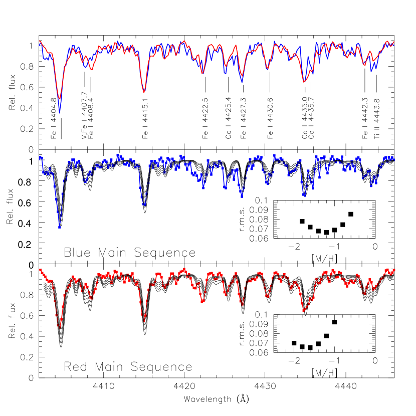
Figure 2: The average bMS (blue line) and rMS (red line) spectra are overplotted in the upper panel, where a few relevant spectral lines are also indicated. Though a few lines (e.g. Fe I 4404.8, Ti II 4443.8) are clearly different in the two spectra, the effect on the line strength due to the difference in metal content between the bMS and rMS stars is partially compensated by the temperature difference (see also Fig. 6). The average bMS (middle panel) and the average rMS (lower panel) spectra are compared with synthetic spectra for different metallicities ([M/H] = $-$1.6, $-$1.4, $-$1.2, and $-$1.0 for the bMS; [M/H] = $-$2.0, $-$1.8, $-$1.6, $-$1.4, and $-$1.2 for the rMS). In these two last panels, observed spectra are represented by colored lines and dots; synthetic spectra are the thin solid lines.

The region 4405–4445 Å  was selected for the comparison of the observed and synthetic spectra, because it contains numerous metallic lines (mainly due to Fe-peak elements, with a few strong Ca and Ti lines), but few lines due to molecules (CH and CN), and no strong H lines, as shown by the upper panel of Fig. 2, where we over-plot the average bMS and rMS spectra. The synthetic spectra were smoothed to the resolution of the observed spectra. Our best values are those that minimize the r.m.s. scatter of the residuals between the observed and synthetic spectra. Using a solar spectrum from the literature, we verified that this procedure accurately reproduces the solar abundance. The results are shown in Fig. 2 (middle and lower panels); the best values are [M/H] $=-1.57$ for the rMS, and [M/H] $=-1.26$ for the bMS. Internal errors of $\pm 0.1$ dex in these abundances were estimated by comparing the values obtained from each half of the wavelength range separately. Systematic errors are dominated by uncertainties in the adopted temperatures: a change of 100 K in the effective temperatures causes a change of $\sim 0.2$ dex in the derived abundances. Note that the temperature uncertainty affects mainly the absolute metallicities, and has much less effect on their difference.

Fig. 2 clearly shows that the bMS stars are more metal rich than the rMS ones. (Note that the differences are made less apparent by the fact that the bMS stars have a higher temperature.) The [Fe/H] of the rMS is consistent with the peak of the abundance distribution of red giants in $\omega$ Cen (Suntzeff & Kraft 1996; Norris et al. 1996), while the bMS corresponds roughly to the second peak in the distribution obtained by those authors. Also, the relative number of stars in the two sequences is consistent with the relative numbers in the RGB, as noted by B04.

3.2 C, N, and Ba abundances

Carbon abundances were obtained by comparing the averaged spectra for the red and blue main sequences with synthetic spectra (Fig. 3) of the spectral region 4300–4330 Å, including the $\Delta v=0$ strong band heads of the A${}^{2}\Delta$-X${}^{2}\Pi$ transition of CH, computed with appropriate model-atmosphere parameters and different values of the C abundances. From this comparison, we found values of [C/M] = 0.0 for both sequences.

Nitrogen abundances were found by a similar comparison (Fig. 4) for the region 4200–4225 Å, including the $\Delta v=-1$ band heads of the X${}^{2}\Sigma$-B${}^{2}\Sigma$  CN transition. A rather large value of [N/M] $\sim 1.0$ or 1.5 was found for the bMS. The N abundance for the rMS is not well constrained: values of [N/M] $\leq 1$  are compatible with observations. Finally, the Ba abundances were obtained from the resonance line of Ba II at 4554 Å. Our values are [Ba/M] = +0.7 and +0.4 for the bMS and rMS, respectively (Fig. 5).

These comparisons show that the bMS is not very rich in C; hence these stars cannot have been formed from the ejecta of C stars. This result becomes relevant when we try to interpret the origin of the chemical anomalies implied by the presence of the bMS (see §6). The Ba abundance for stars on the bMS is compatible with (albeit somewhat smaller than) that observed in metal-rich red giants of $\omega$ Cen (cf. Smith et al. 2000).

4 Individual Spectra and Abundance Spreads

While the $S/N$ of the summed spectra for individual stars is generally low ($\leq$ 10 per pixel along the direction of dispersion), they may provide useful information on the composition of the individual stars. The procedure we followed was the following. First, we re-binned the spectra at a resolution of 2 Å per bin. At this resolution the typical $S/N$ of the spectra is now $\sim 30$, enough for line-index measurements. Second, we measured mean instrumental intensities within a number of narrow spectral bands (see Table 2), centered on strong spectral absorption features as well as in a few reference “pseudo-continuum” spectral ranges. We then derived a number of spectral indices by dividing the instrumental mean intensity measured in the bands containing the features by the weighted average of adjacent “pseudo-continuum” bands. The weights were given by the distances (in wavelength) between the “pseudo-continuum” bands and the bands containing the absorption features. Error bars for these indices were obtained by considering the $S/N$ of the spectra at the wavelength of each band, the bandwidths, and by summing the contributions to errors of both line and “pseudo-continuum” bands. Typical internal errors are 0.059, 0.048, 0.028, 0.030, and 0.029 for H_δ, Ca I 4227, G band, H_γ, and Fe I 4383, respectively.

Figure 6 displays the runs of some of these spectral indices (Fe I 4383, Ca I 4227, and G-band) with the F606W $-$ F814W color for the program stars. Different symbols are used for stars of the bMS and rMS.

The sequences for the bMS stars are nearly as narrow as expected from the internal errors in colors and spectral indices, with the possible exception only of star 3348, which may have a strong G band: this is shown well by Table 3, which compares the spread in line indices (at a given color) expected from internal errors (in colors and spectral indices) with the observed r.m.s. around the best-fitting straight line. The values listed in this table indicate that star-to-star abundance variations within bMS stars have not been detected. By comparing the observed spread with the temperature sensitivity of the spectral features, we may roughly estimate that star-to-star abundance variations within bMS stars are well below 0.08 dex (r.m.s.), with similar values provided by all three indices. The very small abundance spreads for bMS stars that are indicated by line indices agree well with the very small width of the sequence in the color magnitude diagram. We conclude that the bMS is populated by stars having a fairly uniform chemical composition. This might have important implications on its origin.

On the other hand, the rMS stars display star-to-star scatters in the line indices that are much larger than expected from observational errors alone, and larger than those obtained for bMS stars (see Table 3). Note that we omitted from these plots and further comparisons three stars (237, 664, and 3222) having spectra of very low quality. The large spreads are obtained consistently for all metallic spectral indices for the rMS stars. If we compare the excess spread with the expectations based on internal errors, we may roughly estimate that there are star-to-star abundance variations among rMS stars of about 0.15–0.20 dex (r.m.s. scatter), again with similar values provided by all three indices. Such a spread is consistent with the observed width in color of the rMS (about 0.02 mag), which is much larger than that of the bMS (0.008 mag). This value is also consistent with the spread in chemical composition usually found for $\omega$ Cen stars (Suntzeff & Kraft 1996; Norris, Freeman & Mighell 1996), and is therefore not unexpected.

5 Interpreting the observational results

5.1 A super-helium-rich population?

The main result of our investigation is surely the fact that the bMS is $0.3\pm 0.2$ dex more metal rich than the rMS, the error bar being essentially due to uncertainties in the relative temperatures. This definitely removes the possibility raised in B04 that the bMS represents a super-metal-poor population.

The second piece of evidence provided by our spectra, i.e., that the bMS and rMS have the same radial velocity, makes the already remote possibility that the bMS represents a background object even more unlikely. In addition, B04 have shown that the DMS is present from the cluster center to at least 17 arcmin from the center. We also verified that the WFPC2 field at 7 arcmin (Fig. 1c in B04) from the center and the outer ACS field (Fig. 1d in B04) have approximately the same ratio of bMS to rMS stars. Finally, we note that preliminary results by some of us (Anderson 2003, Anderson & King 2005, in preparation) show that the average proper motions of the two populations are indistinguishable.

In summary, all observational evidence indicates that the bMS stars are $\omega$ Cen members. Still, we remain with the puzzling observational result that the bMS stars are more metal rich than the rMS ones. The problem is that any canonical stellar models with canonical chemical abundance tell us that the blue MS should be more metal poor than the red MS.

One of the hypotheses made by B04, and further investigated by Norris (2004) is that the bMS might have a strong He enhancement. Interestingly enough, from his theoretical investigation, Norris (2004) supposed a metal content for the bMS and rMS very similar to the values that we have measured. In view of our observational findings, the He overabundance seems to be the only way to explain the MS split. Though a direct measurement of He for the MS stars is not feasible, we are in a position to test this hypothesis, as we now know the metallicity of both the bMS and the rMS.

Because of the sizable dependence of the CMD location of the MS on the He content, we tried to make an indirect estimate of the He content of the bMS by comparison with suitable stellar models. We used the most updated physics to calculate specific models for the metallicities of the two sequences. We refer to Pietrinferni et al.  (2004) for the details of the models, as well as the adopted physical scenario. Unlike Pietrinferni et al. (2004), however, in the present work we assumed [$\alpha$/Fe] = 0.4; the alpha-enhanced models will be published in a forthcoming paper. As for the adopted initial He content, we assumed a canonical $Y=0.246$ (Salaris et al. 2004) for the $Z=10^{-3}$ metallicity appropriate for the rMS, and we tried $Y=0.248$, $Y=0.35$, and $Y=0.45$ for the metallicity $Z=2\times 10^{-3}$ appropriate for the bMS. The results of the fit are shown in Fig. 7. Clearly, the model with the standard He content cannot fit the bMS. The bMS can be reproduced only by adopting $0.35<Y<0.45$. The ridge line of the bMS is best fitted by an isochrone for $Y=0.38$. Our conclusions are very similar to those of Norris (2004), but they are based on the measured MS metallicities and on more up-to-date stellar models.

5.2 The progeny of the bMS

No such high He abundance has ever been found in any other GC (Cassisi, Salaris, & Irwin 2003, Salaris et al. 2004), though there are a few anomalous clusters that might have He overabundance, as discussed at the end of this Section. Surely, it is not easy to explain its origin (see next Section). Therefore, even if our hypothesis seems robust, we searched for other, independent evidence.

In particular, we looked for the progeny of the bMS He-rich stars. We do not expect to learn much from the red giant branch (RGB), because of its spread in metallicity, but we do expect that a star with $Y>0.35$ will reach the HB with a smaller mass, because of the combined effect of the decrease of the evolving mass (evolutionary lifetimes decrease strongly when the He content increases) and the increase of total mass loss due to the longer RGB lifetime. Its zero age HB location should therefore be on average hotter (bluer) than a HB star with canonical He content (D’Antona et al. 2002, D’Antona & Caloi 2004; see also Sweigart 1997). More specifically, our stellar models predict, for a fixed stellar age and mean mass-loss efficiency, that the mean ZAHB effective temperature increases by $\sim 1500$ K when the He abundance is raised from $Y=0.25$ to 0.35, but it increases by $\sim 15,000$ K when the He abundance changes from $Y=0.25$ to $\sim 0.45$.

Indeed, $\omega$ Cen does have an anomalously blue HB (D’Cruz et al. 2000, Momany et al.  2004), extending to a temperature corresponding to stars which must have almost completely lost their envelope. The extended HB of $\omega$ Cen  shows a clear discontinuity at $T_{\rm eff}\sim 20,000$ K, as is clearly visible in the $U$, $U-V$ CMD of Fig. 2 in Momany et al. Also D’Cruz et al. find a discontinuity at a similar temperature (gap G3 in their notation), in a far-UV CMD. From the CMD of Momany et al., we estimate that at least 17% of the HB stars in $\omega$ Cen  are hotter than the $T_{\rm eff}=20,000$ K discontinuity (hereafter extremely-hot HB stars, EHB). The counts are not complete in the faint (hotter) part of the HB in that $U$, $U-V$ CMD. On the other hand, D’Cruz et al. estimate that 32% of the stars are hotter than the same discontinuity. In their diagram these stars are the brightest stars, while some incompleteness is surely present in the counts of the cooler (fainter) stars in their F160W, F160W $-$ $V$ CMD. In conclusion, we estimate that between 20% and 30% of the HB stars of $\omega$ Cen are hotter than the discontinuity located at $T_{\rm eff}\sim 20,000$ K. Interestingly enough, in the ACS field at 17 arcmin from the center, we estimate that $24\pm 3$% of the MS stars are in the bMS. It is therefore tempting to associate the EHB stars in $\omega$ Cen with the progeny of the bMS, He-rich stars. Norris (2004) also came to a similar conclusion. The EHB stars need not necessarily include all the progeny of the bMS, because of the dispersion in the mass loss during the RGB phase, but the star counts and the presence of the discontinuity seem to indicate that most of them could be on the EHB. It might also be relevant that Moehler et al. (2002) have found the hottest HB stars ($T_{\rm eff}>30,000$ K) to have a supra-solar He content. Moehler et al. interpret this anomalously high He abundance as the effect of the extra mixing in late He-flash stars (Brown et al. 2001). If our hypothesis is correct, at least part of the He enhancement could be primordial. An easy test of this idea would be the measurement of the He content for HB stars with $T_{\rm eff}<30,000$, which should not experience the extra mixing, according to the Brown et al. (2001) models. We are presently investigating whether other EHB GCs show evidence of a double or broadened MS.

The He content also affects the HB luminosity, in the sense that a higher helium content would imply a brighter HB. In this respect, Norris (2004) pointed out that a higher helium content for the more metal-rich population in the bMS of $\omega$ Cen seems to be contradicted by the results of Butler, Dickens, & Epps (1978), and Rey et al. (2000), who find that the RR Lyraes with $-1.3<$[Fe/H]$<-1.0$ are on the average fainter than the more metal-poor ones by 0.2–0.3 magnitude (though there are at least two very bright, likely evolved, metal-rich RR Lyraes). However, as discussed above, it is reasonable to assume that if the HB stars of the metal-rich population are very rich in He, most of them must be hotter than the instability strip, and therefore, as pointed out by Norris (2004), the RR Lyraes cannot be representative of the entire cluster population. Hints of a brighter HB than expected (from models) for $\omega$ Cen are visible in Fig. 2 of Momany et al. (2004), where the HB of OmCen from $\sim 6,000$ K to $>30,000$ K is shown. While the HB luminosity of $\omega$ Cen needs further investigation, it is surely interesting to note that two of the most massive GCs of our Galaxy, NGC 6388 and NGC 6441, both have HBs that are still enigmatic, both because of the presence of an extended blue tail (Rich et al.  1997) despite their metallicities ([Fe/H] = $-0.6$ and $-0.5$, respectively), and because they are populated by anomalously bright RR Lyraes (Pritzl et al.  2002, 2003). Moreover, these two clusters have a tilted HB, with the blue side brighter than the red one (Rich et al. 1997, Raimondo et al. 2002). Interestingly enough, Sweigart & Catelan (1998), in order to explain the HB anomalies of NGC 6388 and NGC 6441, proposed a helium value $Y=0.38$–0.43 (very similar to the helium enhancement we need to explain the bMS of $\omega$ Cen). Also, M13 is well known to have an anomalously bright and extended HB, brighter than the HB of a cluster with very similar metallicity like M3. Johnson & Bolte (1998) and Paltrinieri et al. (1998) have shown that the anomalous HB of M13 cannot be due to an age effect. Johnson & Bolte interpret the difference between the HBs of M13 and M3 as due to a higher ($\Delta Y\sim 0.05$) helium content in M13. There are a number of (indirect) evidences in the literature that there could be populations of stars with an enhanced helium content in GCs, and this effect needs to be investigated in more detail.

6 Discussion

If an extremely high helium content is the explanation of the abnormal bMS of $\omega$ Cen, the immediate question that arises is: Where does all this He come from? Most authors try to explain the abundance spread within $\omega$ Cen as a peculiar chemical evolution history for this object, which possibly was once the nucleus of a dwarf galaxy (for a comprehensive discussion of the literature, see Gratton, Carretta, & Sneden 2004). In this framework, the enormous production of He is attributed to pollution by the ejecta of a well-defined group of stars. If we compare the bMS and rMS abundances, the difference of helium abundance required to explain our data is about $\Delta Y=0.14$, while the analogous variation in heavy metal content is $\Delta Z<0.002$ (assuming that the variation of abundances of the Fe-peak elements is representative of all metals). The $\Delta Y/\Delta Z>70$ suggested by these data is more than an order of magnitude larger than the value found appropriate for Galactic chemical evolution (see, e.g., Jimenez et al. 2003). It is possible that the mass of $\omega$ Cen was just right to allow the ejecta of high-mass supernovae to escape, while retaining the ejecta of SNe whose progenitors were $\sim 10$ $M_{\sun}$. This could explain $\omega$ Cen’s unique chemical evolution, as explained below.

Within a similar scenario, we are forced to look for stars which produce He very efficiently. The first obvious candidates are intermediate-mass stars, which according to various authors (see, e.g., Izzard et al.  2004) may indeed produce large amounts of He, which can pollute the surrounding nebula during the AGB phase. However, the amount of ejected He does not seem to be enough to raise $Y$ to the values needed to explain the bMS. Moreover, these same stars should also produce C efficiently; the fact that we found a similar C abundance for both the rMS and bMS stars (see §3) seems to exclude this possibility.

Norris (2004) suggested that massive ($\sim 20$ $M_{\sun}$) stars can be the source of the high He content. However, while it is conceivable that heavier elements collapse into the central black hole, we do expect that a large amount of ejected He would be accompanied by a corresponding large amount of CNO and other $\alpha$-elements such as Mg and Si.. This fact seems to be contradicted by the observational evidence described in §3.2. An appealing alternative may be represented by the smallest among core-collapse supernovae (SNe). According to the prescriptions by Thielemann, Nomoto, & Hashimoto (1996), complemented by data by Argast et al. (2002), SNe with initial masses smaller than about 10–14 $M_{\sun}$  produce significant amounts of He, while producing only small amounts of heavier elements. According to the same authors, the ejecta of a 10 $M_{\sun}$ star might indeed have $\Delta Y/\Delta Z\sim 70$, enough to explain the difference between the bMS and the rMS of $\omega$ Cen. Among the other elements considered in this paper, we notice that models by Thielemann et al. (1996) predict that N is more abundant in the ejecta of the less massive core collapse SNe with respect to more massive ones, while C abundances increase with increasing progenitor mass; these predictions agree qualitatively with our observations. On the other hand, there is no prediction about Ba in these SN models. Ba is observed to be overabundant in metal-rich stars of $\omega$ Cen, with a pattern characteristic of the s-process (see Smith et al. 2000). AGB stars are supposed to produce most of the s-process elements, though it is possible that massive stars make a small contribution. Our data suggest a moderate overabundance of Ba in the bMS stars; this fact must still be confronted with adequate nucleosynthetic predictions.

There are two additional problems which need to be taken into account by any model of the stellar population history in $\omega$ Cen. The first one, already raised by Norris (2004), is that in order to elevate $Y$ from 0.24 to $\sim$0.38 one has to assume that most, if not all the material from which the bMS stars formed is made up of the ejecta of the first generation of stars. The second problem is that these ejecta, which must necessarily come from a large number of stars (in view of the size of the bMS stellar population), must have been well homogenized in their metal content before the stars of the bMS formed, as shown by the homogeneity found for the bMS in §4.

Table 1: Observed bMS and rMS stars

ID	RA(2000)	DEC(2000)	F606W	F606W-F814W
		bMS
0530	13:25:26.605	-47:38:48.06	20.37	0.79
0577	13:25:26.945	-47:39:18.22	20.71	0.83
0718	13:25:28.177	-47:41:31.60	20.60	0.82
0795	13:25:27.834	-47:38:29.77	20.37	0.79
1416	13:25:31.581	-47:41:12.63	20.50	0.81
1616	13:25:32.108	-47:39:35.49	20.74	0.85
1993	13:25:33.688	-47:38:45.38	20.62	0.83
2522	13:25:36.322	-47:38:41.99	20.63	0.83
2529	13:25:37.045	-47:41:38.78	20.14	0.75
2739	13:25:37.772	-47:40:59.10	20.69	0.85
2822	13:25:37.952	-47:40:20.87	20.29	0.79
2938	13:25:38.026	-47:38:52.49	20.78	0.86
3256	13:25:39.718	-47:40:43.15	20.64	0.83
3348	13:25:40.197	-47:41:18.56	20.39	0.77
3977	13:25:42.130	-47:39:11.94	20.04	0.74
3990	13:25:41.996	-47:38:26.85	20.83	0.87
4085	13:25:42.438	-47:38:46.17	20.14	0.76
		rMS
0179	13:25:25.223	-47:40:09.27	20.36	0.85
0237	13:25:25.767	-47:41:12.67	20.22	0.83
0568	13:25:27.303	-47:41:05.85	20.45	0.86
0571	13:25:27.259	-47:40:52.00	20.61	0.90
0664	13:25:27.526	-47:39:57.83	20.53	0.88
0851	13:25:28.477	-47:39:47.50	20.20	0.81
1259	13:25:30.480	-47:39:44.94	20.09	0.78
1350	13:25:30.625	-47:38:25.99	20.52	0.87
1475	13:25:31.389	-47:39:20.16	20.54	0.89
1677	13:25:32.794	-47:41:22.78	20.67	0.88
1980	13:25:33.925	-47:40:11.67	20.26	0.83
2294	13:25:35.745	-47:40:20.30	20.11	0.80
2900	13:25:38.425	-47:41:09.22	20.14	0.79
3080	13:25:38.871	-47:40:13.00	20.28	0.84
3222	13:25:39.779	-47:41:37.65	20.45	0.84
3533	13:25:40.434	-47:39:26.57	20.55	0.88
4302	13:25:43.376	-47:39:01.88	20.44	0.87

Table 2: Spectral bands used for spectral indices

Feature	Min. Wavelength	Max. Wavelength
	Å	Å
Cont.	4051.0	4061.0
Hδ	4094.0	4112.0
Ca I 4227	4224.0	4230.0
Cont.	4231.0	4236.0
Cont.	4278.5	4286.0
G-band	4294.5	4318.0
Hγ	4334.5	4349.0
Cont.	4356.0	4364.0
Fe I 4383	4380.0	4387.6
Cont.	4440.0	4448.0

Table 3: Spreads in line indices

	Expected	bMS	rMS
Fe I	0.031	0.033	0.063
Ca I	0.050	0.061	0.071
G-band	0.030	0.030	0.053

Figure 1: The observed H_γ line in the average bMS (upper panel) and rMS (lower panel) spectra is compared with the synthetic spectra for different temperatures (5000, 5200, 5400, 5600, 5800, and 6000 K). Gravities and metal abundances in the models were chosen to be compatible with the final adopted values.

Figure 3: The average bMS (upper panel) and the average rMS (lower panel) spectra are compared with synthetic spectra in the region 4301–4339 Å, including the band-heads of the CH-band. Synthetic spectra were computed for atmospheric parameters appropriate for the stars, and C abundances of [C/M] = $-0.5$, 0, and +0.5 dex. Thick solid lines are the observed spectra, thin lines are the synthetic spectra.

Figure 4: The average bMS (upper panel) and the average rMS (lower panel) spectra are compared with synthetic spectra in the region 4200–4225 Å, including the band-heads of the $\Delta v$ = 2–0 violet CN band. Synthetic spectra were computed for atmospheric parameters appropriate for the stars, [C/M] = 0, and N abundances of [N/M] = 0, 0.5, 1.0, and 1.5 dex. Thick solid lines are the observed spectra, thin lines are the synthetic spectra.

Figure 5: The average bMS (upper panel) and the average rMS (lower panel) spectra are compared with synthetic spectra in the region of 4544–4564 Å, including the resonance Ba II line at 4554 Å. Synthetic spectra were computed for atmospheric parameters appropriate for the stars, and Ba abundances of [Ba/M] = $-0.5$, 0, 0.5, and 1.0 (upper panel), and [Ba/M] = $-0.5$, 0, and 0.5 (lower panel). Thick solid lines are the observed spectra, thin lines are the synthetic spectra.

Figure 6: Runs of various spectral indices (upper panel: Fe I 4383; middle panel: G band; and lower panel Ca I 4227) with the F606W $-$ F814W color for the program stars. Filled and open symbols are bMS and rMS stars, respectively. Internal error bars are also shown for comparison.

References

- (1) Anderson, J. 1997, PhD Thesis, UC Berkeley
- (2) Anderson, J. 2003, in ASP Conf. Ser. 296, “New Horizons in Globular Clusters Astronomy”, ed. G. Piotto, G. Meylan, S. G. Djorgovski, & M. Riello (San Francisco: ASP), p. 125
- (3) Anderson, J., & King, I. R. 2005, in preparation
- (4) Argast, D., Samland, M., Thielemann, F. K., & Gerhard, O. E. 2002 , A&A, 388, 842
- (5) Bedin, L. R., Piotto, G., Anderson, J., Cassisi, S., King, I. R., Momany, Y., & Carraro, G. 2004a, ApJ, 605, L125 [B04]
- (6) Bedin, L. R., Cassisi, S., Castelli, F., Piotto, G., Anderson, J., Salaris, M., Momany, Y., & Pietrinferni, A. 2004b, MNRAS, submitted
- (7) Brown, T. M., Sweigart, A. V., Lanz, T., Landsman, W. B., & Hubeny, I. 2001, ApJ, 562, 368
- (8) Butler, D., Dickens, R. J., & Epps, E. 1978, ApJ, 225, 148
- (9) Castelli, F., Gratton, R. G., & Kurucz, R. L. 1997, A&A, 318, 841
- (10) Cassisi, S., Salaris, M., & Irwin, A. W. 2003, ApJ, 588, 862
- (11) Cassisi, S., Schlattl, H., Salaris, M., & Weiss, A. 2003, ApJ, 582, L43
- (12) D’Antona, F., Caloi, V., Montalbán, J., Ventura, P., & Gratton, R. 2002, A&A, 395, 69
- (13) D’Antona, F., & Caloi, V. 2004, ApJ, 611, 871
- (14) D’Cruz, N., et al. 2000, ApJ, 530, 352
- (15) Gratton, R. G., Carretta, E., & Sneden, C. 2004, ARA&A, 42, 385
- (16) Hilker, M. & Richtler, T. 2000, A&A, 362, 895
- (17) Izzard, R. G., Tout, C. A., Karakas, A., & Pols, O. R. 2004, MNRAS, 350, 407
- (18) Jimenez, R., Flynn, C., McDonald, J., & Gibson, B. K. 2003, Science, 299, 1552
- (19) Johnson, J. A., & Bolte, M. 1998, AJ, 115, 693
- (20) Kurucz, R. L. 1992, CD-ROM 13
- (21) Lee, Y. W., Joo, J. M., Sohn, Y. J., Rey, S. C., Lee, H. C., & Walker, A. R. 1999, Nature, 402, 55
- (22) Moehler, S., Sweigart, A. V., Landsman, W. B., & Dreizler, S. 2002, A&A, 395, 37
- (23) Momany, Y., Bedin, L. R., Cassisi, S., Piotto, G., Ortolani, S., Recio Blanco, A., De Angeli, F., & Castelli, F. 2004, A&A, 420, 605
- (24) Norris, J. E. 2004, ApJ, 612, 25
- (25) Norris, J. E., & Da Costa, G. S. 1995, ApJ, 447, 680
- (26) Norris, J. E., Freeman, K. C., & Mighell, K. J. 1996, ApJ, 462, 241
- (27) Paltrinieri, B., Ferraro, F. R., Carretta, E., & Fusi Pecci, F. 1998, MNRAS, 293, 434
- (28) Pancino, E., Ferraro, F. R., Bellazzini, M., Piotto, G., & Zoccali, M. 2000, ApJ, 534, L83
- (29) Pietrinferni, A., Cassisi, S., Salaris, M., & Castelli, F. 2004, ApJ, 612, 168
- (30) Pritzl, B. J., Smith, H. A., Catelan, M., & Sweigart, A. V. 2002, AJ, 124, 949
- (31) Pritzl, B. J., Smith, H. A., Stetson, P. B., Catelan, M., Sweigart, A. V., Layden, A. C., & Rich, R. M. 2003, AJ, 126, 1381
- (32) Raimondo, G., Castellani, V., Cassisi, S., Brocato, E., & Piotto, G. 2002, ApJ, 569, 975
- (33) Rey, S. C., Lee, Y. W., Joo, J. M., Walker, A., & Baird, S. 2000, AJ, 119, 1824
- (34) Rich, R. M. et al. 1997, ApJ, 484, L25
- (35) Salaris, M., Riello, M., Cassisi, S., & Piotto, G. 2004, A&A, 420, 911
- (36) Smith, V. V., Suntzeff, N. B., Cunha, K., Gallino, R., Busso, M., Lambert, D. L., & Straniero, O. AJ, 119, 1239
- (37) Suntzeff, N. B., & Kraft, R. P. 1996, AJ, 111, 1913
- (38) Sweigart, A. W. 1997, ApJ, 474, L23
- (39) Sweigart, A. V. & Catelan, M. 1998, ApJ, 501, L63
- (40) Thielemann, F. K., Nomoto, K., & Hashimoto, M., 1996, ApJ, 460, 408