Spallation dominated propagation of Heavy Cosmic Rays and the Local Interstellar Medium (LISM)

Measurements of ultra heavy nuclei at GeV/n energies in the galactic cosmic radiation address the question of the sources (nucleosynthetic s- and r-processes). As such, the determination of CR source abundances is a promising way to discriminate between existing nucleosynthesis models. For primary species (nuclei present and accelerated at sources), it is generally assumed that the relative propagated abundances, if they are close in mass, are not too different from their relative source abundances. Besides, the range of the correction factor associated to propagation has been estimated in weighted slab models only. Heavy CRs that are detected near Earth were accelerated from regions that are closer to us than were the light nuclei. Hence, the geometry of sources in the Solar neighbourhood, and as equally important, the geometry of gas in the same region, must be taken into account. In this paper, a two zone diffusion model is used, and as was previously investigated for radioactive species, we report here on the impact of the local interstellar medium (LISM) feature (under-dense medium over a scale $\sim 100$ pc) on primary and secondary stable nuclei propagated abundances. Going down to Fe nuclei, the connection between heavy and light abundances is also inspected. A general trend is found that decreases the UHCR source abundances relative to the HCR ones. This could have an impact on the level of r-process required to reproduce the data.

1 Introduction

Beyond the iron peak, the flux of Cosmic Ray nuclei drops by several orders of magnitude. The UHCRs require peculiar environments to be nucleosynthesised and two distinct processes are involved: very generally, either the neutron flux in the medium is low so that the neutronic capture rate is less than the $\beta$-decay rate of nuclei, or the flux is high (capture rate much greater than $\beta$-decay rate); these two situations are commonly referred to as s- (slow) and r-process (rapid). The situation is obviously more complex –  see Meyer (1994) for an illuminating review –. One particular issue is the determination of the relative contributions of s- and r-process nucleosynthesis required to explain the data, inferring the corresponding source abundances from the elemental and isotopic abundances.

Based on model predictions (Meyer 1994) as well as on some analysis of CR data (Brewster et al. 1983), it is shown, for example, that for $Z\geq 89$, the entire Solar System abundances must be attributed to the r-process. On the opposite, the latter does not contribute to $Z\leq 40$ (Binns et al. 1981). In-between, most of the elements exist as a mixture of r- and s- contributions. Their origin (e.g., massive stars, explosive nucleosynthesis) and exact abundances are still debated (Goriely 1999; Cowan & Sneden 2004) and CRs could provide some answers. However, to determine the CR source abundances, the fluxes measured near Earth must be propagated back through the Galaxy, which is not a straightforward task.

We shall not discuss here the important question of the time elapsed since nucleosynthesis and propagation which is studied through radioactive heavy elements (Thielemann et al. 2002) and which is another part of the puzzle, nor shall we use any propagation network to study all the abundances (Letaw et al. 1984). We instead focus on propagation. The goal of this paper is to demonstrate the importance of the local CR-source distribution and in particular to examine the effect of the local gas distribution on calculations of source abundances from data. As a matter of fact, whereas the truncation of path lengths for UHCRs has been discussed (through the weighted slab approach) and recognised as having a large impact on the propagation of UHCRs (Clinton & Waddington 1993; Waddington 1996), we illustrate here how this truncation is realised as a deficit in nearby sources in the two zone diffusion model. The low density gas in the local interstellar medium (LISM) is also of particular importance. It is shown that this under-dense region leads to results different from both the standard two zone diffusion model (which is equivalent to a simple leaky box model) and the truncated weighted slab.

The main results of this study are: i) around a few GeV/n, the relative abundance of $Z>60$ nuclei to the lighter ones is decreased when the LISM features are taken into account – the strength of the effect is inversely related to the value of the diffusion coefficient (i.e. to the energy) and is directly related to the destruction cross section values (i.e. to $Z$) –; ii) the shape of the spectra at low energies is sensitive to the value of the diffusion coefficient, providing a way to determine the latter as it breaks the propagation parameter degeneracy (Maurin et al. 2002) observed in standard diffusion model (i.e., with constant gas and source disk distribution); iii) in the UHCR context of relative abundance determination (Pb/Pt and Actinides/Pt), a gas sub-density has a major effect for mixed species (species with both primary and secondary contributions) only.

In $\S 2$, we give some simple arguments which allow us to understand why the local sub-density is expected to have a major influence on heavy CRs at GeV/n energies. In $\S 3$, the model taking into account the sub-density as a circular hole is exposed. Profiles in the LISM cavity as well as spectra for primary and secondary-like nuclei under various source geometry assumptions are compared to those obtained in a standard “no-hole” diffusion model. The correction factors used to determine the source abundances are then derived and consequences for the data are discussed in $\S 4$. We then conclude and comment on further developments demanded by UHCRs propagation.

2 Why a local sub-density may affect the propagation

It has been previously recognised than very heavy nuclei have a peculiar propagation history compared to light nuclei. This is related to their large destruction cross sections which make them have very short path lengths. Regarding this extreme sensitivity to nuclear destruction, an UHCR breaks-up more often than a lighter one and thus propagates for a shorter distance. Kaiser et al. (1972) emphasized that the strength of the source and its location in space and time may be a dominant local contribution or merely adds to the general background depending on whether this source is close or far. These authors use a very simple model in which propagation starts from a single source in space and time. They conclude that $A>81$ elements cannot be explained by any source older than $10^{6}$ yr. In the present paper, the steady-state approximation is however assumed but the spatial discreteness hypothesis is relaxed to some extent. This is a first step away from a leaky box model towards a more realistic description. The framework is a two zone diffusion model (thin disk and halo) which has been used by many authors for light nuclei, e.g. Maurin et al. (2001). In particular, such a model has distinct features compared to leaky boxes. The interstellar matter density is now located in a thin disk with CRs spending most of their time in the diffusive halo. The characteristic times of the various processes in competition during propagation (see below) can be extracted (Taillet & Maurin 2003). As it is shown below, the fact that the typical distances travelled by heavy or UHCRs before their destruction could be as little as a few hundreds of pc naturally means that LISM properties are an important ingredient for propagation.

2.1 Propagation characteristic times vs A

During the propagation of nuclei through the Galaxy, several processes affect their journeys. All of these have specific time/length scales which characterise the importance of the considered process relative to the others. The nuclei can undergo energy losses of different forms, interact with atoms of the ISM and be destroyed in a spallation process or escape from the boundaries of the diffusive volume (i.e. the galactic halo) because of the combined influences of diffusion and convection.

In a leaky box model, the density of gas in the box is constant so that the link between characteristic lengths and times is simple and the comparison to the escape length straightforward. In reality, spallation and energy losses occur when a nucleus crosses the galactic disk. Thus, the characteristic times (or lengths) for those processes are directly linked with the number of disk-crossings (Taillet & Maurin 2003) which should be compared to the diffusive and convective escape times.

2.1.1 Spallation dominates over energy losses

Whether in a leaky box model or a more sophisticated model as used here, spallations and losses both occur when gas is traversed. We assume its density to be $n_{\rm{ISM}}=1$ cm^-3. The spallation rate is given by $\Gamma_{\rm sp}=n_{\rm{ISM}}\sigma v$, where $v$ is the velocity of the nucleus and $\sigma$ is the reaction cross section. For this study, the Letaw et al. (1983) cross sections are accurate enough ($E_{k/n}$ is the kinetic energy per nucleon):

$$\sigma=\sigma_{\infty}[1-0.62\exp(-E_{k/n}/200)\sin(10.9E_{k/n}^{-0.28})]\,,$$

$$\sigma_{\infty}(\rm{E_{k/n}>2GeV/n})=45A^{0.7}[1+0.016\sin(5.3-2.63\log(A))]\,.$$

The loss rate is given by $\Gamma_{\rm{loss}}=\left(dE/dt\right)_{\rm{loss}}/E_{k}$, where $E_{k}$ is the kinetic energy of the nucleus, and the Coulomb and ionisation energy losses are taken into account (Mannheim & Schlickeiser 1994; Strong & Moskalenko 1998) assuming the ionised fraction of the ISM to be 0.033. In both cases, $dE/dt$ is proportional to $Z^{2}$, with $Z$ the charge of the nucleus.

At a given $E_{k}/n$, $\Gamma_{\rm sp}$ scales with the atomic mass $A$ as $A^{0.7}$ ($\log A$ does not induce strong variations). Assuming $A=2Z$, which is not the case for heavy nuclei ($A>2Z$), ionisation and Coulomb loss rates also increase with A but following $\Gamma_{\mathrm{ion/coul}}\propto A$. A comparison of these two rates yields at 1 GeV/n

$$\Gamma_{\mathrm{sp}}\sim 10\times(A/10)^{-0.3}\;\Gamma_{\mathrm{ion}},$$

$$\Gamma_{\mathrm{sp}}\sim 60\times(A/10)^{-0.3}\;\Gamma_{\mathrm{coul}}.$$

This means that the effect of spallation is always dominant over energy losses (at higher energy the effect is even stronger). The latter are thus discarded in the rest of this paper as it mainly focuses on qualitative effects. Note also that the cross sections have not been corrected for the effects of decay which can be significant for the propagation of heavy nuclei. These effects, as well as energy losses and reacceleration, will be properly taken into account in a separate paper where $\beta$-decay and electronic capture decay will be re-examined in the context of the present diffusion models.

2.1.2 Time scales of diffusion, convection and spallation

Once established that spallations are dominant relative to the energy losses, we compare the former to the convection and diffusion processes taking into account the number of disk-crossings in the two zone diffusion model. For further justification and details the reader is referred to Taillet & Maurin (2003).

It is well known that $\tau_{\rm{diff}}=L^{2}/K(E)$ is the characteristic escape time needed by a nucleus to leave a diffusive volume of size $L$ for a diffusion coefficient $K(E)$. The presence of a galactic wind (velocity $V_{c}$), assumed to be constant and perpendicular to the galactic plane, induces a general convective motion throughout the Galaxy. Considering that the diffusive process is still present, the boundary to be taken into account is not the halo size but the distance for which the diffusion cannot compete anymore with the convection and brings the nucleus towards the Earth. With this consideration, one can define the typical time scale for the convection escape process as $\tau_{\rm{wind}}=2K(E)/V_{c}^{2}$.

Spallation only occurs within the disk of total thickness $2h$. The typical length associated with the spallation process in a diffusive propagation is $r_{\rm{sp}}=K(E)/(h\Gamma_{\rm{sp}})$. The time scale, assuming a purely diffusive transport is then $\tau_{\rm{sp}}=r_{\rm{sp}}^{2}/K(E)=K(E)/(h\Gamma_{\rm{sp}})^{2}$.

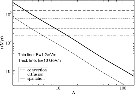
Figure 1: Characteristic times of diffusive/convective escape and spallation as a function of the atomic mass. Typical values $K_{0}=0.0112$ kpc²Myr^-1 and $L_{\rm{halo}}=4$ kpc were considered. The times have been calculated at kinetic energies per nucleon of 1 GeV/n and 10 GeV/n in the two zone diffusion model.

The characteristic times for diffusion, convection and spallation are plotted on Fig. 1 as a function of the atomic mass of the nucleus $A$ at two different kinetic energies per nucleon (1 GeV/n and 10 GeV/n). As we assume $K(E)=K_{0}\beta(\mathcal{R}/1\rm{GeV})^{\delta}$ (where $\mathcal{R}$ is the rigidity), the convection and diffusion times are constant with A. At 1 GeV/n, it appears that spallation is almost always dominant, except for the very light nuclei where both convection and diffusion compete. At 10 GeV/n, spallation is less dominant but remains the major process for the heavier nuclei. A naive (and false) interpretation of these figures is that a heavy nucleus never escapes from the Galaxy. Actually, many paths lead from the source to the halo boundary and these numbers only indicate the typical time a CR reaching our position can have travelled before being destroyed. For convection and diffusion, $\tau_{\rm{diff}}$ and $\tau_{\rm{wind}}$ define an exponential cutoff whereas the cutoff is smoother for spallation (Taillet & Maurin 2003).

Table 1 contains the typical spallation distances for different atomic masses (10, 50, 100 and 200) and a set of three diffusion coefficients (two extreme values and one median) which fit the B/C ratio when combined with the appropriate choice for the other propagation parameters (Maurin et al. 2001, 2002). For A=100 and A=200 and for the median value of the diffusion coefficient, the spallation length scales have the same order of magnitude as the size of the observed local gas sub-density (see Sect. 3). This sub-density precludes the creation of secondary species in the local bubble and the average density crossed by a primary or a secondary nucleus during its journey is smaller than when this sub-density is not taken into account. It is expected that heavier nuclei will be more sensitive than lighter nuclei to this feature.

A	Group		$K_{0}$ (kpc2 Myr-1)
		0.0016	0.0112	0.0765
10	LiBeB/C	210 pc	1.25 kpc	6.38 kpc
50	Sub-Fe/Fe	70 pc	390 kpc	2.01 kpc
100	Z=44-48	40 pc	250 pc	1.27 kpc
200	Actinides	30 pc	150 pc	780 pc

Table 1: Typical length scales of the spallation process for different nuclei and diffusion coefficients at 1 GeV/n.

The smaller the spallation length scale, the greater the effect of the sub-density is expected to be and this suggests that the local bubble must be considered to treat the heavier species. This reasoning is valid only if the cosmic rays undergo the same diffusive process in the LISM than in the rest of the Galaxy. There is at least two indications supporting this assumption:

• The local bubble and the galactic halo share some common properties. Hence, it seems reasonnable that the values of the diffusion coefficient in both regions are not drastically different. As we use only one coefficient for the disk and the halo, the latter can be seen as an effective value that also applies for the local bubble.

• The second clue comes from the analysis of secondary radioactive species which can travel for a few hundreds of pc only before decaying. Ptuskin & Soutoul (1998) were able to derive the corresponding ’local’ diffusion coefficient modelling the LISM as three shells of gas with various densities. They found a larger value at low energy than the standard one found from B/C analysis. This again points towards a diffusive transport of CRs in the local bubble.

3 Two zone model with a hole

Firstly, the local interstellar medium (LISM) is known to be a highly asymmetric low density region, extending between 65 to 250 pc – recent studies have for the first time conducted tomography of the LISM (Lallement et al. 2003) –. As a consequence, the spallation rate is lessened so that the primary fluxes are expected to be enhanced.

Secondly, the history of the origin of the local bubble (see Breitschwerdt & Cox (2004) for a review) is an imprint of the explosive stellar activity in the Solar neighbourhood (Maíz-Apellániz 2001; Berghöfer & Breitschwerdt 2002; Benítez et al. 2002). The spatio-temporal position of these sources is certainly of importance. However, as the steady state is assumed in this paper, only the spatial influence can be inspected. For example, Lezniak & Webber (1979); Webber (1993) have shown that an absence of nearby sources (in a diffusion model) can truncate the path lengths in weighted slab models. This truncation has been recognised to be of great importance in the propagation of heavy nuclei (Clinton & Waddington 1993; Waddington 1996). This effect is realized here as a circular hole of a few hundreds of pc surrounding the Solar area reflecting the fact that no very recent sources have exploded in the Solar neighbourhood. Note that this truncation could also be an effect of the matter traversed during the acceleration and the escape from a source region.

3.1 The model

The effects of a local sub-density on radioactive species have been studied in the context of a diffusion model by Donato et al. (2002). As it is difficult to derive an analytical solution of the diffusion equation using a realistic distribution for the gas, it is assumed that the LISM is a circular cavity of radius $a$ (see below). It appeared that the radioactive flux received on Earth was lessened by $\sim$35% when the decay length of the radioactive species was twice the size of the sub-density compared to the case when a sub-density was not taken into account (cf. Donato et al. (2002), Fig. 4). Furthermore, in order to match measured radioactive abundance ratios (${}^{10}\rm{Be}/^{9}\rm{Be}$, ${}^{26}\rm{Al}/^{27}\rm{Al}$ and ${}^{36}\rm{Cl}/\rm{Cl}$), the size of the local sub-density was constrained to lie within 60 and 100 pc – values consistent with direct observations. This increases confidence in the model. In the latter, the Galaxy is considered as a thin disk where the sources and gas are located (Fig. 2). To be consistent with the results obtained for light stable nuclei (Maurin et al. 2001), for radioactive nuclei (Donato et al. 2002) and also for antiprotons (Donato et al. 2001), the same geometry is used. The width of the disk, $2h$, is 200 pc and the Galactic radius $R$ is 20 kpc. The exact value for $R$ is not important so that one can set the center of the cylindrical geometry at the Earth position (see Donato et al. (2002)), which simplifies the calculations. The diffusive halo, empty of gas and sources, extends to a height $L$ on each side of the disk which can vary from 1 to 10 kpc. The local sub-density is then a hole of radius $a$ in this disk, whereas the source sub-density is a hole of radius $b$. From the disk emerges a galactic wind with a constant velocity $V_{c}$ that adds a convective component to the diffusive propagation of the CRs.

These assumptions (sources and gas in a thin disk, circular hole, halo empty of gas, same diffusion coefficients in the disk and in the halo) are probably too strong. However, they have lead to a successful description of many species in a consistant way, an issue we think to be of great importance. We also believe that the approximations made (some that would need a heavy numerical treatment to be relaxed) would have a minor effect compared to the one induced by the LISM geometry. Despite many weaknesses, the present diffusion model has to be thought as a first step towards a more realistic description.

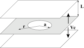
Figure 2: Schematic view of the cylindrical geometry for the model used in this paper: the hole region of radius $a$ is located in a thin disk surrounded by a diffusive halo of size $L$ (a convective wind $V_{c}$ may be present). The exact radius of the Galaxy radius $R$ is not important (see text).

Energy losses are not taken into account meaning that in this cylindrical geometry the diffusion equation reads

$$-K\Delta N+V_{c}\frac{\partial N}{\partial z}+2h\Gamma\delta(z)N=q(r,z)\delta(z)$$ (1)

where $N=N(r,z)$ is the differential density in energy. The Dirac distribution $\delta(z)$ expresses the fact that the sources and the gas are only located in the thin disk. In this work, the results are always normalized to the source spectrum thus the only quantity one must specify is $q(r)$, the radial source distribution (cf. A.1). It is appropriate to use a decomposition in Bessel space to solve this equation and the complete derivation is given in detail in Appendix A (the derivation closely follows that given in Donato et al. (2002)).

The height $L$ of the halo is a free parameter as are the galactic wind velocity $V_{c}$, the spectral index $\delta$, and normalization $K_{0}$ of the diffusion coefficient. Those parameters must be tuned to fit the data. In the following work and when mentioned, the max, median and min set of parameters can be understood as detailed in Table 2. These three sets are the two extreme and median sets (with regard to the value of the diffusion coefficient normalization) shown to be compatible with B/C analysis. Eventually, throughout the paper, the gas sub-density is set to $a=100$ pc whereas the sub-density in sources can be varied.

set	$\delta$	$K_{0}$ (kpc2 Myr-1)	$L$ (kpc)	$V_{c}$ (km s-1)
max	0.46	0.0765	15	5
med	0.7	0.0112	4	12
min	0.85	0.0016	1	13.5

Table 2: Two extreme and one median sets of parameters shown compatible with B/C analysis (Maurin et al. 2001).

In the remainder of this section, we focus on the differences between a model with a hole in the surrounding gas (and/or sources) and the standard diffusion model with no hole. Note that as the propagation parameters used for the standard diffusion model (with no hole) are fitted to B/C, the results obtained in this latter model and those obtained in a LB are similar (see Fig. 8). It is useful to define the “enhancement factor” which is defined as the ratio of a given hole configuration to the standard diffusion model (no hole, hereafter SDM) for a given set of propagation parameters. Such a ratio ensures that the source spectral shape and normalization are factored out for primaries and the production cross section is for secondaries. The discussion of the absolute effects on abundances – including the standard result from the leaky box model – is contained in Sect. 4.

3.2 General behaviour

To separate the effects of the absence of gas and sources in the hole, we study three different configurations: i) in the first case, only the gas is absent from the “hole region” but the sources are still present, ii) the second case is the opposite configuration and the hole is a sub-density of sources but not of gas and iii) finally, we consider the situation where there is both a hole in gas and a hole in sources (possibly having different sizes).

3.2.1 Profiles

Figure 3: Left panels: Fe-group. Right panels: Actinide group. Primaries (upper), secondaries (middle) and sec/prim (lower) enhancement factors are plotted as a function of the distance to the center of the sub-density (the fluxes are normalized relatively to the SDM fluxes). In both models, the hole in gas and the hole in sources are equals $a=b=0.1$ kpc and $E_{k}$/n=1 GeV/n. The set of astrophysical parameters is the median set: $K_{0}=0.0112$ kpc² Myr^-1, $L=4$ kpc, $V_{c}=12$ km s^-1 and $\delta=0.7$.

The enhancement factors for primaries, secondaries and for the ratios Secondary/Primary are plotted on Fig. 3 as a function of the distance to the center $r$ ($r=0$ corresponds to Earth location). The three hole configurations described above have been studied. For these profiles, the size of the hole is 0.1 kpc, and the median set of parameters has been used, namely: $K_{0}=0.0112$ kpc² Myr^-1, $L=4$ kpc, $V_{c}=12$ km s^-1 and $\delta=0.7$. The iron group (left panel) and the actinide group (right panel) are both considered at 1 GeV/n. Firstly, it appears that when the distance from the hole is large enough (typically $3a$), the enhancement factor tends to unity (i.e. there is no difference from the no-hole case) emphasing that, in a first approximation, the hole has only a local effect. An important consequence is that nuclei are not sensitive to other density features of the ISM, which justifies the crude model used here.

When a hole in gas only is considered, more primaries (upper panels) are expected (i.e., enhancement factor $>1$) compared to the SDM as nuclei entering the hole region do not undergo spallation as they would if gas were present. In that case, at the Earth location, there is a 60% increase in primaries of the iron group and a 275% increase in the actinides. In the opposite configuration (sources absent, gas present), no primary nuclei are produced within the sub-density and those which have propagated to the hole undergo spallation. In that case, the primary density is lessened compared to the SDM ($\sim$ 20% for Fe-group nuclei and $\sim$ 40% for actinides).

The third case, where both gas and sources are absent from the hole region is found to give intermediate results. It appears that in this geometry the absence of gas has a larger impact that the absence of sources: for a hole in gas and sources, the enhancement factor is greater than unity. There is a 20% effect for nuclei of the iron group and a 75% effect for actinides. However, the result is quite sensitive to the particular geometry assumed. To obtain a very rough estimate of this sensitivity, the diffusion equation was solved for a spherical geometry where sources and gas holes were taken as shells. In this latter configuration (which is unrealistic, but which may be considered as the extreme opposite geometry to that of the thin disk case) the enhancement and relative importance of a hole in gas or a hole in sources are smaller and the gas-hole enhancement is almost cancelled by a hole in sources.

When looking at the secondary enhancement factor (Fig. 3, middle panels), a sub-density in sources only has almost no consequences ($\sim$ 10% effect) on the secondary flux (enhancement factor $\sim$ 1). This indicates that most of the secondaries found in the solar neighbourhood originate from primaries that were not produced locally. When a gas hole is considered (close sources are present), the secondary enhancement factor is maximal ($\sim 80$% for Fe-group nuclei and $\sim 450$ % for actinides). In this case, the secondaries present at $r=0$ cannot have been produced locally (as there is no gas) and have all been propagated from further regions. Once they reach the gas sub-density, they cannot be destroyed, which explains the enhancement. The enhancement in the case of a hole in gas and sources is explained in the same manner. However, this enhancement is slightly lower ($\sim 60$% for Fe-group nuclei and $\sim 350$% for actinides) than the case in which only gas is excluded: when sources are present in the hole, primaries from the hole can propagate in the disk and produce secondaries that may diffuse back towards the Earth.

3.2.2 Spectra

Enhancement factor spectra for primaries, secondaries (Fe-group nuclei in the left panel and actinides in the right panel) and for the ratio Sec/Prim are plotted in Fig. 4 between 500 MeV/n and 100 GeV/n at $r=0$. At high energy the behaviour of any hole configuration tends, as expected, to the no-hole case at high energies as spallation becomes negligible. In the case of a sub-density in gas, the enhancement factor for the median propagation configuration is quite large (almost a factor of 2), even for the Fe flux. Comparatively, the sub-Fe/Fe ratio is enhanced by a mere 20%.

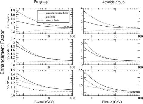
Figure 4: Same as Fig. 3 but for spectra at $r=0$.

Actually, these enhancements, whether for primaries or secondaries, are not very sensitive to the exact value of $L$ and $V_{c}$ (because the enhancements are normalized to the SDM). They mostly depend on the value of the diffusion coefficient. Hence, it implies, for example, that a very precise measurement of the iron abundance spectrum would give some hint as to the value of the diffusion coefficient, by evaluating the deviation from a standard diffusion model. The larger the deviation at low energy, the smaller the diffusion coefficient required to fit the deviation.

3.3 Other dependences

3.3.1 Enhancement factor vs $r_{\rm sp}$

It is useful now to display the enhancement factor as a function of $a/r_{\rm sp}$ ($a$ being the size of the hole and $r_{sp}$ the typical spallation distance, see Sect. 2.1.2). As several combinations of $(K_{0}$, $\delta)$ for a given choice of $A$ yield the same $r_{\rm sp}$ (Taillet & Maurin 2003), the parameter dependence is more economically studied. Indeed, to quickly obtain the enhancement due to a hole in gas – or any combination of holes, compared to the SDM – it is sufficient to take the desired $K_{0}$ and $\delta$, choose a specific $A$ and evaluate $r_{\rm sp}$ for a given energy. The enhancement factor is then directly inferred from Fig. 5. Two cases are displayed to emphasize the effect of the Galactic wind: the first with $V_{c}=0$ km s^-1 and the second with $V_{c}=12$ km s^-1. This is the typical range of the possible values for the wind. It is not a dominant effect.

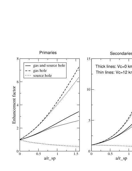
Figure 5: Primary and secondary enhancement factors as a function of the ratio $a/r_{\rm sp}$ for the median set of parameters. The size of the holes are $a=b=0.1$ kpc, and the different values of $r_{\rm sp}$ cover a wide range of energies, $K_{0}$ and destruction cross section values.

The enhancement factor for several nuclei could be obtained from the previous plot, but for simplicity, they have been gathered for light to heavy nuclei for several energies and propagation sets in Table 3. Despite the fact that the three sets of propagation parameters have been shown to be compatible with B/C analysis, the minimal set gives some unrealistic enhancement factors. This allows the exclusion of an unrealistic configuration for which the diffusion slope required to fit the B/C data was 0.85 (Maurin et al. 2002), far away from any theoretical expectations. Actually, in previous papers attempting to obtain some conservative value for the propagation parameters from the sole B/C and sub-Fe/Fe ratios (Maurin et al. 2001, 2002), the hole configuration has not been taken into account. In order to be able to firmly exclude some $K_{0}$ and $\delta$ values, a new detailed analysis is required, which goes beyond the scope of this paper. In conclusion, it seems that very small values of $K_{0}$ have to be excluded because of the too large enhancement they yield when a hole in gas is included.

	Prim	Sec
	min/med/max	min/med/max
LiBeB-CNO
E=1 GeV/n	2.08/1.17/1.03	2.29/1.13/1.02
E=5 GeV/n	1.36/1.07/1.02	1.33/1.05/1.01
E=10 GeV/n	1.21/1.04/1.02	1.19/1.03/1.01
Fe-group
E=1 GeV/n	6.24/1.58/1.11	20.9/1.75/1.11
E=5 GeV/n	2.34/1.23/1.06	3.38/1.26/1.06
E=10 GeV/n	1.71/1.15/1.04	2.03/1.16/1.04
Z=44-48
E=1 GeV/n	8.67/1.80/1.14	43.0/2.14/1.15
E=5 GeV/n	2.95/1.31/1.08	5.06/1.36/1.08
E=10 GeV/n	1.99/1.19/1.06	2.59/1.22/1.06
Actinides
E=1 GeV/n	17.6/2.77/1.26	200/4.45/1.31
E=5 GeV/n	5.73/1.61/1.15	18.2/1.82/1.16
E=10 GeV/n	3.28/1.37/1.11	6.22/1.46/1.12

Table 3: Enhancement factors at the Earth’s location due to the presence of a local sub-density on four groups of nuclei. Different energies (from 500 MeV/n to 10 GeV/n) and three sets of parameters have been considered.

3.3.2 Impact of the hole in sources $b$

A few decades ago, some authors introduced the possibility of a truncation of the path lengths used in the weighted slab formalism. Lezniak & Webber (1979) then showed that a hole in sources in a diffusion model mimics such path-length truncation. This truncation was first introduced to fit best the sub-Fe/Fe ratio, though afterwards, new results on cross section production reduce the need for it. However, truncation was implemented for UHCR propagation and it has a sizeable effect (Clinton & Waddington 1993; Waddington 1996), especially for secondary nucleus production. The truncation uncertainty is here equivalent to the uncertainty in $b$ (see also Fig. 8 in Sec. 4.3).

In this section, the hole in sources varies from $b=0$ to $b=500$ pc. In Fig. 6, the enhancement factors of primaries and secondaries of the iron group and actinide group are plotted as function of the size of the hole in sources. The energy of the nuclei is 1 GeV/n and the size of the gas hole is once again fixed at $a=100$ pc (because this feature is certainly present). Depending on the hole size $b$, one can have an enhancement factor that is greater or lower than unity. Actually, this situation occurs only because the hole in sources is in competition with the hole in gas.

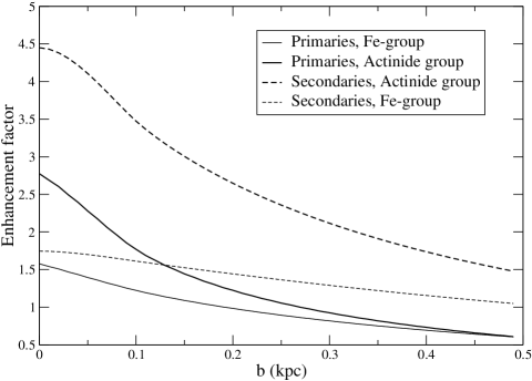
Figure 6: Enhancement factor for primaries and secondaries of the Fe and actinide groups as a function of the size of the hole in sources, $b$. A constant gas hole radius $a=100$ pc was considered and the propagation computed using the median set of parameters.

However, we do not wish to put too much emphasis on this effect. It must be considered as an illustration of the impact on relaxing the condition of continuous distribution of sources. The limits of our model are reached and to go further, one must relax the steady state approximation. In fact, the question of nearby sources cannot be easily disconnected to the question of recent sources (Taillet et al. 2004).

3.4 Preliminary conclusions

Setting holes in a diffusion model affects the abundance spectra, especially at low energies where the importance of spallation is larger. A hole in gas increases the number of primaries, even more the number of secondaries. Conversely, a hole in sources decreases the number of primaries (the secondaries being quite insensitive to it). So there is a balance between the two configurations. Unless a large hole in sources is chosen ($b\gtrsim 300$ pc), because the hole in gas (size $a\sim 100$ pc) is firmly established – from direct observations, and also indirectly because it better fits light radioactive CRs measurements (Donato et al. 2002) –, the final effect is an enhancement of the cosmic ray fluxes.

The dependence of this enhancement to the halo size $L$ and the convective wind $V_{c}$ is minor. The main dependence is through the diffusion coefficient, $K(E)$. The previous sections helped us to establish that very small diffusion coefficients that were found to best fit the B/C ratio in a standard diffusion model (Maurin et al. 2002) must be discarded as they produce a too large enhancement of fluxes when the hole in gas is taken into account. It is reassuring since these small values for $K_{0}$ corresponded to quite large diffusion slopes, unsupported by theoretical considerations (too far from a Kolmogorov or a Kraichnan turbulence spectrum). However, a new study of B/C must be conducted taking into account the hole configuration to provide a quantitative result. Going one step further, one sees that the low energy secondary fluxes can be useful to determine $K_{0}$. The secondaries better suit this estimation than primaries as, unlike the latter, they are not very sensitive to a hole in sources. This could provide another way, apart from using radioactive nuclei (Ptuskin & Soutoul 1998), to extract the diffusion coefficient without too much ambiguity. Note also that the heavier the nucleus, the more local it is, so that looking at different nuclei gives different sampling regions where the diffusion coefficient is averaged. Figure 7 in the next section will provide a better understanding of how the effect of the hole sometimes disconnects from the dependence on $L$ and so in certain configuration why the flux at low energy only depends on $K_{0}$ (if the latter is not too large).

One can now come to the differences in derived source abundances. Cosmic ray fluxes are propagated to source by using a leaky box (or equivalently a standard diffusion model) and hole models applied to real data.

4 Consequences for CRs observations

UHCR abundance spectra have been obtained via spacecraft measurements since the 1970s, most notably by ariel 6 (Fowler et al. 1987), heao-3 (Binns et al. 1989), trek (Westphal et al. 1998) and the Ultra-Heavy Cosmic-Ray Experiment (or uhcre; Donnelly et al., in preparation).

The data are scarce, especially in the actinide region, and only elemental abundances have been obtained. However, several important conclusions have already been drawn. They are related i) to nucleosynthesic aspects (see the introduction), ii) to the possible site of acceleration and iii) to the mechanisms leading to elemental segregation during acceleration.

The recent results of uhcre provide unprecedented statistics and will allow to give firmer conclusions. However, as emphasized throughout this paper, some aspects of the propagation still need to be clarified in order to fully interpret these data. In this last section, some questions and results about UHCRs are first reiterated, before inspecting the propagation effects on these nuclei in different models. In particular, those species suffering from major propagation uncertainties (regardless of cross-sections, which is another issue) are sorted.

4.1 Introduction: UHCR data, their interpretation and general issues

The ultra-heavy ($Z>70$) elemental abundance ratios most pertinent in determining cosmic ray origin are Pb-group/Pt-group, ₉₂U/₉₀Th and Actinides/Pt-group.

The first, Pb/Pt, provides clues as to biases in the CR-source abundances. Elements in the Pt-group are mainly intermediate-FIP, refractory and r-process, while in the Pb-group low-FIP, volatile and primarily s-process elements predominate. Thus an anomalous GCR Pb/Pt ratio (relative to Solar values) would show up any nucleosynthetic (s- or r-process) or atomic (FIP or volatility) bias in the source abundances. This ratio is more enlightening than (for example) the Pt/Fe or Pb/Fe ones, as the ratios of nuclei similar in mass, are supposed to be relatively unaffected by interstellar propagation. This point is discussed in the next section. In common with other space-based measurements, the uhcre results (Donnelly et al., in preparation) demonstrate that the Pb/Pt abundance ratio is decidedly low in the GCRs ($0.24\pm 0.03$) compared to the best estimates from solar and meteoritic material ($1.03\pm 0.12$; Lodders (2003)). Even assuming a very severe propagation effect on this ratio ($\times 2.6$), the GCR value is a mere $0.63\pm 0.09$. This could indicate a volatility-based acceleration bias as Pb elements are relatively volatile (Ellison et al. 1997; Meyer et al. 1998).

The relative abundance of chronometric pairs such as ₉₀Th and ₉₂U can provide an estimate of the time elapsed since their nucleosynthesis. Most models of actinide decay indicate that ₉₂U/₉₀Th drops to unity about 1 Gyr after nucleosynthesis. However, only 44 actinides have been detected so far. 35 of these were detected by the uhcre and this experiment provides the only estimate yet of the ₉₂U/₉₀Th in the CRs. The 1$\sigma$ upper limit is only $\sim 1$, implying that significant ₉₂U decay has occurred and that the time elapsed since nucleosynthesis is relatively large. The transuranics can also be used as excellent cosmic ray ’clocks’ since the relative abundances of ₉₃Np, ₉₄Pu and ₉₆Cm fall drastically 107 yr after nucleosynthesis (Blake & Schramm 1974). Again, the best data available are from the uhcre, which detected one ₉₆Cm event. The longest-lived isotope of Cm has a half-life of only 16 Myr. This fact, combined with the ₉₂U/₉₀Th results from the same experiment suggests that the CR-source material is an admixture of old and freshly-nucleosynthesised matter, such as that found in superbubbles.

Finally, anomalies in the Actinides/Pt ratio could indicate an unusual, possibly freshly-nucleosynthesised component in the cosmic ray source matter. Results from all of the space-based measurements indicate a high value relative to solar system material, though the uncertainties on the latter are large. The uhcre’s Actinide/Pt ratio ($0.028^{+0.006}_{-0.005}$) in broad agreement with other observations, is higher than in the present interstellar medium ($0.014\pm 0.002$) and similar to that of the protosolar medium ($\sim 0.023$) and the interior of superbubbles ($0.029\pm 0.005$). These observational values are unadjusted for propagation and so are therefore best considered as lower-limits.

There are large uncertainties on the effects of propagation on these ratios. For example, estimates of the effects of propagation on Pb/Pt vary from factors as low as $\times 1.3$ to as high as $\times 2.6$. Accurate estimates of propagation effects are therefore crucial to interpret the data.

4.2 UHCR abundances and the correction factor for the propagation

As emphasized above, in the context of UHCRs, one issue is the determination of relative source abundances of, for example, Actinides/Pt and Pb/Pt. To this end, in this subsection, it is verified that the choice of a more refined propagation model leaves the abundance ratio of close heavy nuclei (if considered as being pure primaries) almost unchanged. Figure 7 shows that for any hole configuration and any propagation parameters, the maximum effect on the Actinides/Pt ratio (when both considered as pure primaries) is at most 20% (as obtained in the source hole case). The effect is even smaller for the Pb/Pt ratio (also considered as pure primaries). However, Pt is a mixed species and is responsible for the uncertainties on these two ratios. Considering for example the ratio $\rm{Pt}^{sec}/\rm{Pb}^{prim}$, the difference in Pt production from Pb in the various hole model can be as large as a factor of 2. Hence, this hole must be taken into account using a complete propagation network to derive abundances in a model that is thought to be more realistic than the LB model.

Figure 7 is also useful in understanding the propagation regimes of heavy nuclei. For very small diffusion coefficients (equivalent to low energies), the spallation length is much smaller than the halo size. In that case, the ratio of two close nuclei is independent of $L$ but sensitive to any hole. Conversely, for large diffusion coefficients (equivalent to high energies), the spallation length is much larger than the hole size, thus, the ratio is only sensitive to $L$. Depending on the nucleus and energy under consideration, one can be in an intermediate regime where both the hole and halo influence the ratio.

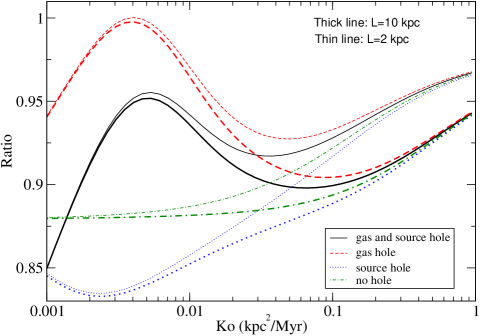
Figure 7: ${\rm\{Actinides/Pt\}}_{\rm propag.}/{\rm\{Actinides/Pt\}}_{\rm source}$ ratio (all species considered as pure primaries). For large diffusion coefficients, the effect of the hole (any configuration) is negligible and only depends on the halo size $L$: the curves with the same $L$ tend to the same values – upper (resp. lower) group of curves: $L=2$ kpc (resp. $L=10$ kpc). On the other hand, for low diffusion coefficients, the ratio is completely insensitive to $L$. See text for details.

4.3 Abundance normalization bias vs A

The ariel 6 experiment (Fowler et al. 1987) measured the abundances of Fe-group elements so that they provided abundances normalized to Fe. One peculiar feature is the overabundance of the $44\leq Z\leq 48$, $62\leq Z\leq 69$ and $70\leq Z\leq 74$ groups which are presumed to be predominantly secondary in origin. Actinides were also found to be overabundant in this experiment. Later, in Binns et al. (1989), CR abundances (from heao 3) were propagated back using a LB model. This study rises the possibility that a bias occurs during the process because the propagation correction factor in a LB may be incorrect.

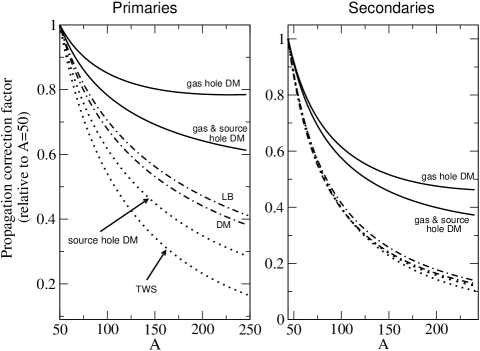
Figure 8: Propagation correction factor for a given $A$ relative to the nucleus $A=50$. From the curves, one directly gets $q_{0}^{\rm Model\leavevmode\nobreak\ 1}/q_{0}^{\rm Model\leavevmode\nobreak\ 2}={\rm Corr.Factor}^{\rm Model\leavevmode\nobreak\ 2}/{\rm Corr.Factor}^{\rm Model\leavevmode\nobreak\ 1}$ which is the relative CR abundances obtained using different propagation models. The standard DM and the LB model (2 dash-dotted lines) are equivalent. The hole source DM and the TWS (2 dotted lines) which predict a smaller primary density than the LB are also equivalent. Left panel is for primaries, right panel for secondaries (it is assumed for simplicity that these secondaries come from the parent $A_{\rm prim}=A_{\rm sec}+6$). See text for discussion.

Figure 8 gives the correction factor according to the propagation scheme used. As before, for primaries, it corresponds to the flux divided by the source term whereas for secondaries, it corresponds to the flux divided by the production cross section. All the results are normalized to the iron group ($A\sim 50$). For the diffusion models (without hole and with different hole configurations), the median set of parameters is used ($K_{0}=0.0112$ kpc² Myr^-1). We also plotted the results of a LB model and for a truncated weighted slab (TWS). The densities in the TWS are calculated using the escape mean free path and path length distribution (PLD) from Clinton & Waddington (1993) – detail can be found in appendix B. The truncation was taken to be 1 g cm^-2: Waddington (1996) showed that such a truncation combined with a pure $r$-source better fitted the UHCR abundances.

There is a general trend showing that the propagation in a LB (or as well as in a standard diffusion model) predicts larger fragmentation of nuclei than a diffusion model with a hole in gas, especially for high A. For a larger diffusion coefficient, this effect would be weaker. Note that the effect is stronger for secondaries (right panel) than for primaries (left panel), as already discussed. Furthermore, it has to be noticed that both the TWS model and the source hole diffusion model give lower primary densities that a LB or a standard DM model. This is pointing towards the study of Lezniak & Webber (1979) who showed that a truncation of the short path lengths was equivalent to the removal of the nearby sources in a DM. As an illustration (not displayed here), we find that to obtain the same curve with the source hole diffusion model or with the WS model truncated at $x_{0}=1$ g cm^-2, the size of the hole has to be set around 180 pc (when using the median diffusion coefficient).

As the energy of the events measured in the detectors are not well known, the propagation correction cannot be easily performed. As explained in the caption of the figure, these curves give rough corrections to transform LB-derived source abundances to the “more realistic” ones in hole models. For illustrative purpose, we apply this correction to the LB abundances obtained by Binns et al. (1989). Figure 9 shows that for the specific CR abundances obtained by these authors, the LB-propagated abundances (open triangles) display a discrepancy compared to the SS ones above $Z=60$, namely that they are twice larger. Previously, a possible enhancement in the r-process contribution in this charge range was suggested. Applying the approximate correction due to a gas sub-density in our diffusion model, a better agreement with SS abundances is obtained (filled triangles) for heavier species while lighter species are less affected. One must bear in mind that this is a very rough estimation.

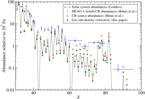
Figure 9: Circles: Solar System abundances (Lodders 2003). Squares: Measured CR abundances combining HEAO and Ariel data (Binns et al. 1989). The open up triangles represent the CR source abundances using a Leaky Box model from the above data. Filled down triangles are these values corrected by the factor between the LB model to a diffusion model with a hole in gas. These factors are taken from Fig. 8, and correspond to the median propagation set. For the ranges $44\leq Z\leq 48$, $62\leq Z\leq 69$, $72\leq Z\leq 74$, the nuclei were considered to be pure secondaries.

5 Conclusion

The propagation of heavy to UHCRs was considered in a two zone diffusion model with various assumptions about the local gas density and source distribution. The propagation parameters used here were previously shown to be compatible with B/C and antiproton data, which allows a coherent treatment of both heavy and lighter species. Moreover, a previous analogous study for radioactive species has validated the relevance of modelling the observed local sub-density as a circular hole of $\sim 100$ pc in the Galactic disk, increasing confidence in the model used here.

It is well known that for light nuclei, Leaky Box and diffusion models are equivalent, which is not the case for the radioactive species. Using propagation parameters matching B/C ratio in a LB and a DM, we explicitly checked that the same equivalence exists for the heavy nuclei. However, this equivalence does not hold when a local sub-density in gas and/or sources is taken into account. These new models can be understood as physical configurations which change the path length distribution. They are equivalent to truncation – whose importance has previously been underlined for the propagation of heavy nuclei – for the case of a hole in sources. To our knowledge, there is no well-know modified PLD corresponding to the case of a hole in gas.

It was found that for nuclei in the same mass range, these models have a weak impact on estimates of CR abundances as long as one deals only with pure primaries and pure secondaries. The determination of mixed species abundances, e.g. Pt, is on the other hand very sensitive to the presence of a local gas sub-density. The strength of this effect depends strongly on the diffusion coefficient value (and hence on the energy of the CRs).

Whereas this effect is small for propagated nuclei of similar masses, it becomes important when considering the whole range of nuclei from iron to the actinides. For a typical diffusion coefficient, it is found that the CR abundances derived in a gas hole model are lessened by a factor of 2 compared to those evaluated in a LB model. In this case, the discrepancy with solar abundances for $Z>60$ nuclei is smaller. This could have important consequences on the of r-process contribution needed to explain the measured data. Note that all these results were derived independently of the value of the production cross sections.

Further work – using a full propagation network for nuclei – is required to obtain more quantitative results. Before this work to be completed, a similar study will first be conducted for nuclei that are unstable to electronic capture: the latter are known to affect source abundances (see e.g., Table I in Letaw et al. (1985)) and the local subdensity is likely to have an effect (slightly different than the one observed for $\beta$-unstable nuclei) on their propagation.

Appendix A Derivation in cylindrical geometry

The calculation leading to the solutions for the two zone model in cylindrical geometry without energy losses is presented and follows Donato et al. (2002). The diffusion equation describing the evolution of the nucleus density $N(r,z)$, including spallation and convection due to the galactic wind reads:

$$-K\Delta N(r,z)+V_{c}\frac{\partial N}{\partial z}+2h\Gamma\delta(z)N(r,z)=q(r,z)$$

where $q(r,z)=q(r)\times 2h\delta(z)$ is the source distribution, $K$ is the diffusion coefficient, $V_{c}$ is the velocity of the galactic convection wind, $h$ is the thickness of the disk, and $\Gamma=n\sigma v$ is the spallation reaction rate. The Dirac distribution is needed as the spallation and sources are only present in the disk. Considering a local density with a radius $a$, the density is then given by $n=n_{ISM}\Theta(r-a)$, where $\Theta(r-a)$ is the Heavyside function. The space of the Bessel functions is well adapted to this geometry and we use the following decompositions, with $\zeta_{i}$, the $i$-th zero of the Bessel function $J_{0}$:

$$N(r,z)=\sum_{i}N_{i}(z)J_{0}\left(\zeta_{i}\frac{r}{R}\right)$$ (2)

$$q(r)=\sum_{i}q_{i}J_{0}\left(\zeta_{i}\frac{r}{R}\right)$$

$$\Theta(r-a)N(r,z)=\sum_{i}\Omega_{i}J_{0}\left(\zeta_{i}\frac{r}{R}\right)$$

with $\Omega_{i}$ following

$$\Omega_{i}=\frac{2}{J_{1}^{2}(\zeta_{i})}\int_{a/R}^{1}\rho N(\rho,0)\Theta(\rho-\frac{a}{R})J_{0}(\zeta_{i}\rho)\rm{d}\rho\;.$$

In the space of Bessel functions, the diffusion equation becomes

$$\frac{\partial^{2}N_{i}}{\partial z^{2}}-\frac{V_{c}}{K}\frac{\partial N_{i}}{\partial z}-\frac{\zeta_{i}^{2}}{R^{2}}N_{i}-\frac{2h\Gamma}{K}\delta(z)\Omega_{i}=-2h\frac{q_{i}}{K}\delta(z)\;.$$ (3)

Using the property of the Bessel functions

$$\int\rho J_{0}(\zeta_{j}\rho)J_{0}(\zeta_{i}\rho)\rm{d}\rho=\left\{\begin{array}[]{ll}\frac{1}{\zeta_{j}^{2}-\zeta_{i}^{2}}[-\zeta_{i}\rho J_{0}(\zeta_{j}\rho)J_{1}(\zeta_{i}\rho)+\\ \zeta_{j}\rho J_{1}(\zeta_{j}\rho)J_{0}(\zeta_{i}\rho)]&\textrm{for $i\neq j$}\\ &\\ \frac{1}{2}\rho^{2}[J_{0}^{2}(\zeta_{i}\rho)+J_{1}^{2}(\zeta_{i}\rho)]&\textrm{for $i=j$}\end{array}\right.$$

$\Omega_{i}$ reads,

$$\Omega_{i}=\left\{\begin{array}[]{ll}\frac{2}{J_{1}^{2}(\zeta_{i})}\frac{a}{R}\sum_{j\neq i}M_{ij}N_{j}&\textrm{for $i\neq j$}\\ &\\ B_{i}N_{i}&\textrm{for $i=j$}\\ \end{array}\right.$$ (4)

with $B_{i}$ and $M_{ij}$ being respectively

$$B_{i}=1-\frac{a^{2}}{R^{2}}\frac{1}{J_{1}^{2}(\zeta_{i})}\left(J_{0}^{2}\left(\zeta_{i}\frac{a}{R}\right)+J_{1}^{2}\left(\zeta_{i}\frac{a}{R}\right)\right)\;,$$

$$M_{ij}=\frac{1}{\zeta_{j}^{2}-\zeta_{i}^{2}}\left[\zeta_{i}J_{0}\left(\zeta_{j}\frac{a}{R}\right)J_{1}\left(\zeta_{i}\frac{a}{R}\right)-\zeta_{j}J_{1}\left(\zeta_{j}\frac{a}{R}\right)J_{0}\left(\zeta_{i}\frac{a}{R}\right)\right]\;.$$

Inserting Eq. (4) in the diffusion equation, Eq. (3) becomes

$$\begin{array}[]{ll}\displaystyle\frac{\partial^{2}N_{i}}{\partial z^{2}}-\frac{V_{c}}{K}\frac{\partial N_{i}}{\partial z}-\frac{\zeta_{i}^{2}}{R^{2}}N_{i}=-2h\frac{q_{i}}{K}\delta(z)&\\ &\\ \displaystyle+\frac{1}{K}\left(2h\Gamma B_{i}N_{i}(0)+4h\Gamma\frac{a}{R}\frac{2}{J_{1}^{2}(\zeta_{i})}\sum_{j\neq i}M_{ij}N_{j}(0)\right)\delta(z)\;.\end{array}$$ (5)

In the halo, the RHS term of Eq. (5) is not present. Considering the boundary condition $N_{i}(z=L)=0$, the solution in the halo is given by

$$N_{i}^{\rm{halo}}(z)=\exp\left(\frac{V_{c}z}{2K}\right)N_{i}(0)\frac{\sinh\left(S_{i}\frac{L-z}{2}\right)}{\sinh\left(\frac{S_{i}L}{2}\right)}\;,$$ (6)

where $S_{i}$ is a constant defined as

$$S_{i}=\left(\frac{V_{c}^{2}}{K^{2}}+4\frac{\zeta_{i}^{2}}{R^{2}}\right)^{\frac{1}{2}}\;.$$

The solution in the thin disk, $N_{i}(0)$, is obtained by integration Eq. (5) across the disk between $z=-h$ and $z=+h$ with $h\rightarrow 0$. Eq. (5) becomes

$$\begin{array}[]{ll}\displaystyle 2N_{i}^{\prime}(0)-2\frac{V_{c}}{K}N_{i}(0)+2h\frac{q_{i}}{K}-\frac{1}{K}2h\Gamma B_{i}N_{i}(0)&\\ &\\ \displaystyle-\frac{1}{K}4h\Gamma\frac{a}{R}\frac{2}{J_{1}^{2}(\zeta_{i})}\sum_{j\neq i}M_{ij}N_{j}(0)=0\;.\end{array}$$ (7)

The continuity between the halo and the disk is established by inserting the halo solution (Eq. (6)) in Eq. (7). Defining $A_{i}$ as

$$A_{i}=V_{c}+KS_{i}\coth\left(\frac{S_{i}L}{2}\right)+2h\Gamma B_{i}$$ (8)

one finds

$$N_{i}(0)=\frac{q_{i}}{A_{i}}2h\left(1-\frac{4\Gamma a}{q_{i}RJ_{1}^{2}(\zeta_{i})}\sum_{j\neq i}M_{ij}N_{j}(0)\right)\;.$$ (9)

It appears that to calculate $N_{i}(0)$, one needs to know the values for all the other orders of the Bessel decomposition. We use a perturbative method to compute these quantities. At the zero-$th$ order, we have $N_{i}^{(0)}(0)=2hq_{i}/A_{i}$, and calculate recursively the $(n+1)$-th order as

$$N_{i}^{(n+1)}(0)=\frac{q_{i}}{A_{i}}2h\left(1-\frac{4\Gamma a}{q_{i}RJ_{1}^{2}(\zeta_{i})}\sum_{j\neq i}M_{ij}N_{j}^{(n)}(0)\right)$$ (10)

until the convergence is reached. In practice, the convergence is reached quite rapidly, after 5 iterations. Using Eq. (2), the density of nuclei in the physical space is then given by

$$N(r,z)=e^{\left(\frac{V_{c}z}{2K}\right)}\sum_{i=0}^{+\infty}N_{i}(0)\frac{\sinh\left(S_{i}\frac{L-z}{2}\right)}{\sinh\left(\frac{S_{i}L}{2}\right)}J_{0}\left(\zeta_{i}\frac{r}{R}\right)\;.$$ (11)

A.1 Primaries and secondaries

The previous derivation is valid for any source term $q(r)$. For the primaries, we consider the two situations where there are sources or not in the hole, but in each case, we assume a constant source distribution $q_{0}$ with $r$. In that case, there are analytical expressions for the components of $q(r)$ in Bessel space, namely

$$q(r)=1\hskip 41.25641pt\rightarrow\;\;\;\;\;q_{i}=\frac{2}{\zeta_{i}J_{1}(\zeta_{i})}$$

$$q(r)=\Theta(r-b)\;\;\;\rightarrow\;\;\;\;\;q_{i}=\frac{2\left(J_{1}(\zeta_{i})-\frac{b}{R}J_{1}(\zeta_{i}\frac{b}{R})\right)}{\zeta_{i}J_{1}^{2}(\zeta_{i})}$$

The secondaries are only produced by spallation of the primary nuclei on the ISM, so their source term is $q(r)=\Gamma_{ps}N^{p}(r)$, where $\Gamma_{ps}$ is the production reaction of the secondaries and $N^{p}(r)$ is the density of primary nuclei. As a consequence, for the secondaries we compute Eq. (9) simply using $q_{i}=\Gamma_{ps}N_{i}^{p}$ where $N_{i}^{p}$, referring to the primaries, have been previously determined.

Appendix B The Truncated Weighted Slab

In this work, we use the truncated weighted slab (TWS) approach as described in Clinton & Waddington (1993). The escape mean free path and path length distribution are defined respectively as,

$$\lambda_{esc}=\left\{\begin{array}[]{ll}5.5\mathrm{\leavevmode\nobreak\ g\leavevmode\nobreak\ cm}^{-2}&\mathrm{for\leavevmode\nobreak\ R}\leq 7.6\mathrm{\leavevmode\nobreak\ GV}\\ &\\ \displaystyle 5.5\times\left(\frac{R}{7.6{\rm GV}}\right)^{-0.4}&\mathrm{for\leavevmode\nobreak\ R\leavevmode\nobreak\ }>7.6\mathrm{\leavevmode\nobreak\ GV}\end{array}\right.$$

and,

$$\mathcal{P}(x)=\left\{\begin{array}[]{ll}\displaystyle\frac{1}{\lambda_{\rm esc}}\exp\left[\frac{x_{0}-x}{x}\right]&\mathrm{for\leavevmode\nobreak\ }x\geq x_{0}\\ &\\ \displaystyle 0&{\rm otherwise}\end{array}\right.$$

where $R$ is the rigidity and $x_{0}$ the truncation of the shortest path lengths ($x_{0}$=1 g cm^-2 in this work). When neglecting the energy losses and assuming only one primary parent $p$ for a secondary $s$, one finds the truncated weighted slab densities of primaries and secondaries to be

$$\begin{array}[]{l}\displaystyle{N_{p}=\frac{\lambda_{p}}{\lambda_{esc}+\lambda_{p}}q_{p}e^{-x_{0}/\lambda_{p}}}\\ \\ \displaystyle N_{s}=\frac{\lambda_{s}\lambda_{p}}{(\lambda_{p}-\lambda_{s})\lambda_{ps}}q_{p}\left[\frac{\lambda_{p}}{(\lambda_{esc}+\lambda_{p})}e^{-x_{0}/\lambda_{p}}-\frac{\lambda_{s}}{(\lambda_{esc}+\lambda_{s})}e^{-x_{0}/\lambda_{s}}\right]\end{array}\;$$

where $\lambda_{p}$ (resp. $\lambda_{s}$) corresponds to the mean free path of a primary (resp. secondary) with respect to its total destruction cross section and where $\lambda_{ps}$ is the mean free path of a primary relatively to the secondary production cross section.

References

- Benítez et al. (2002) Benítez, N., Maíz-Apellániz, J., & Canelles, M. 2002, Physical Review Letters, 88, 081101
- Berghöfer & Breitschwerdt (2002) Berghöfer, T. W. & Breitschwerdt, D. 2002, A&A, 390, 299
- Binns et al. (1981) Binns, W. R., Fickle, R. K., Waddington, C. J., et al. 1981, ApJ, 247, L115
- Binns et al. (1989) Binns, W. R., Garrard, T. L., Gibner, P. S., et al. 1989, ApJ, 346, 997
- Blake & Schramm (1974) Blake, J. B. & Schramm, D. N. 1974, Ap&SS, 30, 275
- Breitschwerdt & Cox (2004) Breitschwerdt, B. & Cox. 2004, astro-ph/0401428, Proceedings of the Conference ”How the Galaxy Works - Galactic Tertulia: A Tribute to Don Cox and Ron Reynolds”, Granada (Spain), 23-27 June 2003, Kluwer (in press), eds. E.J Alfaro, E. Perez, J. Francoastroph
- Brewster et al. (1983) Brewster, N. R., Freier, P.-S., & Waddington, C. J. 1983, ApJ, 264, 324
- Clinton & Waddington (1993) Clinton, R. R. & Waddington, C. J. 1993, ApJ, 403, 644
- Cowan & Sneden (2004) Cowan, J. J. & Sneden, C. 2004, in Origin and Evolution of the Elements, 27–+
- Donato et al. (2001) Donato, F., Maurin, D., Salati, P., et al. 2001, ApJ, 563, 172
- Donato et al. (2002) Donato, F., Maurin, D., & Taillet, R. 2002, A&A, 381, 539
- Ellison et al. (1997) Ellison, D. C., Drury, L. O., & Meyer, J. 1997, ApJ, 487, 197
- Fowler et al. (1987) Fowler, P. H., Walker, R. N. F., Masheder, M. R. W., et al. 1987, ApJ, 314, 739
- Goriely (1999) Goriely, S. 1999, A&A, 342, 881
- Kaiser et al. (1972) Kaiser, T. B., Wayland, J. R., & Gloeckler, G. 1972, Phys. Rev. D, 5, 307
- Lallement et al. (2003) Lallement, R., Welsh, B. Y., Vergely, J. L., Crifo, F., & Sfeir, D. 2003, A&A, 411, 447
- Letaw et al. (1985) Letaw, J. R., Adams, J. H., Silberberg, R., & Tsao, C. H. 1985, Ap&SS, 114, 365
- Letaw et al. (1983) Letaw, J. R., Silberberg, R., & Tsao, C. H. 1983, ApJS, 51, 271
- Letaw et al. (1984) Letaw, J. R., Silberberg, R., & Tsao, C. H. 1984, ApJS, 56, 369
- Lezniak & Webber (1979) Lezniak, J. A. & Webber, W. R. 1979, Ap&SS, 63, 35
- Lodders (2003) Lodders, K. 2003, ApJ, 591, 1220
- Maíz-Apellániz (2001) Maíz-Apellániz, J. 2001, ApJ, 560, L83
- Mannheim & Schlickeiser (1994) Mannheim, K. & Schlickeiser, R. 1994, A&A, 286, 983
- Maurin et al. (2001) Maurin, D., Donato, F., Taillet, R., & Salati, P. 2001, ApJ, 555, 585
- Maurin et al. (2002) Maurin, D., Taillet, R., & Donato, F. 2002, A&A, 394, 1039
- Meyer (1994) Meyer, B. S. 1994, ARA&A, 32, 153
- Meyer et al. (1998) Meyer, J., O’C. Drury, L., & Ellison, D. C. 1998, Space Science Reviews, 86, 179
- Ptuskin & Soutoul (1998) Ptuskin, V. S. & Soutoul, A. 1998, A&A, 337, 859
- Strong & Moskalenko (1998) Strong, A. W. & Moskalenko, I. V. 1998, ApJ, 509, 212
- Taillet & Maurin (2003) Taillet, R. & Maurin, D. 2003, A&A, 402, 971
- Taillet et al. (2004) Taillet, R., Salati, P., Maurin, D., Vangioni-Flam, E., & Cassé, M. 2004, ApJ, 609, 173
- Thielemann et al. (2002) Thielemann, F.-K., Hauser, P., Kolbe, E., et al. 2002, Space Science Reviews, 100, 277
- Waddington (1996) Waddington, C. J. 1996, ApJ, 470, 1218
- Webber (1993) Webber, W. R. 1993, ApJ, 402, 185
- Westphal et al. (1998) Westphal, A. J., Price, P. B., Weaver, B. A., & Afanasiev, V. G. 1998, Nature, 396, 50