Low and intermediate mass star yields: The evolution of carbon abundances

We present a set of low and intermediate mass star yields based on a modeling of the TP–AGB phase which affects the production of nitrogen and carbon. These yields are evaluated by using them in a Galaxy Chemical Evolution model, with which we analyze the evolution of carbon abundances. By comparing the results with those obtained with other yield sets, and with a large amount of observational data, we conclude that the model using these yields combined with those from Woosley & Weaver (1995) for massive stars properly reproduce all the data. The model reproduces well the increase of C/O with increasing O/H abundances. Since these massive star yields do not include winds, it implies that these stellar winds might have a smoother dependence on metallicity than usually assumed and that a significant quantity of carbon proceeds from LIM stars.

1 Introduction

The study of galactic evolution gives important clues about the Universe. The chemical evolution of a galaxy depends mainly on three factors: a) the Initial Mass Function (IMF), b) the Star Formation Rate (SFR), and c) the products ejected to the interstellar medium as a consequence of the stellar evolution. Due to this last ingredient, it is quite important to know the mechanisms of element production in the interior of the stars, where they are produced, in what quantity, and when they are ejected to the interstellar medium. The study of these processes is made through the stellar yields, a concept introduced by Tinsley (1980). Since then, a lot of work has been done in this field to obtain and improve them, first for solar metallicity and then for other stellar metallicities.

Modern studies (Carigi, 2000; Liang, Zhao & Shi, 2001; Chiappini, Romano & Matteucci, 2003, hereinafter CHIA03) have shown that differences in stellar yields reflect appreciable variations in the results obtained with Galaxy Chemical Evolution models. One of the reasons for those differences is our still poor understanding of the evolution of low and intermediate mass (LIM) stars in the post main sequence stages. Another reason is the poor knowledge of the influence of the metallicity on the mass loss by stellar winds. Thus, in spite of the large effort to compute yields, the matter is not clear at all: any improvement in the stellar evolution theory may have an effect on yields, and, therefore, on chemical evolution model results.

For massive stars, one of the most frequently used set of stellar yields has been the one calculated by Woosley & Weaver (1995, hereafter WW). They added to the pre–supernova yields (Woosley & Weaver, 1986) the nucleosynthesis elements produced in supernova type II explosions, for metallicities between $Z=0$ and Z_⊙. Maeder (1992) calculated the yields for stars with mass between 1 M_⊙ and 120 M_⊙, for metallicities in the range from $Z=0.0001$ to Z_⊙, as proceeding from the stellar winds which occur during stellar evolution. Then, Portinari, Chiosi & Bressan (1998, hereafter PCB) obtained massive star yields for the metallicities of the Padova group taking into account all these ingredients: the loss of mass by stellar winds, the influence of the metallicity during stellar evolution and the explosive nucleosynthesis, for computing a complete set of yields. More recently, Limongi, Straniero & Chieffi (2000) and Rauscher et al. (2002) have calculated new massive stars yields, but the mass and/or metallicity range is not so wide as the old yield sets from WW and PCB. As we would like to compare our results with other works we choose only those old yield sets, widely used in the literature.

For the low and intermediate mass star yields, one of the most used sets has been the one obtained by Renzini & Voli (1981) ( hereafter RV), calculated for LIM stars taking into account the effects of convective dredge–up and inner layer burning, the so–called Hot Bottom Burning processes. However, these yields are not successful in predicting the observed abundances C/O and N/O. Some other works such as Marigo, Bressan & Chiosi (1996); Forestini & Charbonnel (1997); Marigo, Bressan & Chiosi (1998) and Van den Hoek & Groenewegen (1997, hereafter VG), or, more recently, Marigo (2001, hereafter MA) have treated the evolution of these last phases in this kind of star. These works compute new sets of stellar yields, which, however, show a very different behavior.

This is the reason why new yields for LIM stars were recalculated (Buell, 1997) using the same basic scheme as RV. Calculations shown and used in this work are based on the study of the transformations that stars with masses between 0.8 and 8 M_⊙ suffer after the Main Sequence, mainly on the thermally pulsing asymptotic giant branch (TP–AGB), when the third dredge—up (TDU) and Hot Bottom Burning (HBB) processes take place. As these processes affect mainly the production of carbon and nitrogen, these yields will have a different behavior in these elements to that found by other authors. We present this new set of yields for metallicities between $log(Z/Z_{\odot})=-0.2$ (or $Z=0.0126$) and $log(Z/Z_{\odot})=+0.2$ ($Z=0.0317$). They are calculated taking into account, as is commonly accepted, that the LIM stars produce primary and secondary components for the CNO elements, and, therefore, these two components are given separately. Besides that, we evaluate these yields by using them as input in a Galactic Chemical Evolution model, and comparing the results with those obtained with other published yield sets, in particular with RV and VK.

There are some recent works (Ventura, D’Antona & Mazzitelli, 2002; Dray et al., 2003) describing detailed evolutionary computations followed from the pre–MS phase up to the very late evolutionary stages for LIM stars, including in particular the AGB phase, and giving the element yields. The problem with using these new sets resides in the incomplete range in mass and Z, necessary for our purposes, due to the large computation time necessary to calculate those models compared with the corresponding one using less exact methods. As we want to compare the results with those obtained by other authors, we prefer to use VG and MA. We check, whenever possible, if differences between our stellar yields and those obtained with more precise methods are significant.

From the observational point of view, there are several open questions about the primary or secondary character of nitrogen and carbon, which have remained unsolved up to now. In particular, for the carbon abundances, the graph of log(C/O) vs O/H shows first a flat line which then increases for oxygen abundances larger than $12+log(O/H)=8$. The flat slope is usually explained as being due to the C mostly being ejected by massive stars with oxygen. However, it is difficult to explain the posterior increase of C/O on the basis of a primary behavior for the two elements. Carigi (2000); Henry, Edmunds & Köppen (2000) and other authors claim that the dependence on metallicity of yields, due mostly to its effect on mass loss by stellar winds in massive stars, is essential for solving this problem, while some others try to explain how a secondary element, proceeding from the carbon ejected by LIM stars, can show this kind of behavior. Here we use new LIM star yields and we will probe their effect on the carbon abundance.

We present the new low and intermediate mass yields in Section 2. Section 3 is devoted to the comparison of the different yield sets used for our purposes, and to explain how to calculate the data sets used as inputs to the chemical evolution model. In Section 4 we summarize the multiphase chemical evolution model and show the resulting calibration for the Milky Way galaxy (MWG). Then the corresponding results for carbon abundances are given. The discussion is given in Section 5 and our conclusions are presented in Section 6.

2 The stellar evolution of LIM along the TP–AGB phase

The evolution after the main sequence (MS) of stars with masses between 0.8 and 8 M_⊙ is determined primarily by the value of their ZAMS mass. The different stages of evolution are described according to the following mass ranges:

• 0.8 M_⊙ – 1.7 M_⊙: During thermal pulses the convective envelope does not penetrate deeply enough to mix processed material into the surface layers, and the composition before and after thermal pulses are the same. The temperature at the base of the envelope between thermal pulses does not get high enough for HBB to occur, therefore there is no change in the composition of these stars during the TP–AGB. They experience a 1^st dredge–up event which modifies the composition of the ejected material. They do not suffer 2^nd or 3^rd dredge–up events.

• 1.7 M_⊙ – 4 M_⊙: Abundances in these stars are dominated by the 3^rd dredge–up, because they undergo many events of this type. The temperature at the base of their envelopes is not high enough to allow HBB, and therefore each dredge–up increases the C and He abundances. The abundance of nitrogen is increased by the first dredge–up.

• 4 M_⊙ – 8 M_⊙: The envelope bases for 4 M_⊙ stars reach a temperature of $\geq 30\times 10^{6}$ K, and then HBB – a CNO cycle at the base of the convective envelope – can take place. The consequence is a decrease of the abundance of carbon and an increase of nitrogen abundance. If there is enough time, it is even possible to convert ${}^{16}O$ to ${}^{14}N$, thus producing a decrease in the oxygen abundance. The ratio N/O will show a severe increase for stars around 4 M_⊙, when the HBB process begins. These stars also typically experience a 2^nd dredge–up which increases their surface helium abundance.

Only a brief summary of the inputs into LIM star models used will be presented here, mostly those details that significantly affect the calculated yields. Additional details can be found in Buell (1997) and Buell, Henry & Baron (2004)

2.1 Luminosity

The luminosity of a TP–AGB star immediately after the first thermal pulse starts at a low value and then grows rapidly during successive pulses until it reaches an asymptotic value. This asymptotic value can be expressed as a function of the core mass and the mass of the star. The asymptotic luminosity of the low–mass stars on the thermally pulsing asymptotic giant branch (TP–AGB) is usually modeled using the core–mass–luminosity relations of Boothroyd & Sackmann (1992).

In recent years, however, it has become apparent that a simple core–mass luminosity relationship (with or without a metallicity dependence) is not appropriate for intermediate mass stars (M$>3.5{{\rm M}_{\odot}}$). The luminosity now appears to depend on the stellar mass as well. Tuchman et al. (1983) showed using semi–analytic arguments that a core–mass luminosity relation holds for AGB stars only when the hydrogen burning shell is separated from the convective envelope. They found that a core–mass luminosity relationship is not appropriate if the convective shell penetrates the hydrogen burning layer. Blöcker and Schönberner (1991) modeled a 7${{\rm M}_{\odot}}$ star and found that it did not follow any kind of core–mass luminosity behavior because the convective envelope penetrated the hydrogen burning layer. This effect has been confirmed by the TP–AGB models of Boothroyd & Sackmann (1992); Lattanzio (1992); Boothroyd, Sackmann & Ahern (1993); Vassiliadis & Wood (1993); Blöcker (1995); Forestini & Charbonnel (1997), and Straniero et.al. (2000).

The asymptotic value of the surface luminosity for stars of all masses is found from:

$$L_{s}=f{\rm L}_{\rm cm}$$ (1)

where

$$f = 1+0.186({\rm M}-2.17),\,\,{\rm M}>2.17{{\rm M}_{\odot}}$$ (2)

$$f = 1,\,\,{\rm M}\leq 2.17{{\rm M}_{\odot}}$$ (3)

M is the total mass of the star ${\rm L}_{\rm cm}$ is the luminosity if a core–mass luminosity relationship were followed, and $f$ is a factor to correct the luminosity for the effects of HBB. This relationship was derived by fitting a function to the AGB models of Boothroyd & Sackmann (1992) and Boothroyd, Sackmann & Ahern (1993). The luminosity depends strongly on mass over 4${{\rm M}_{\odot}}$.

For low–mass stars (${\rm M}<3{\rm M}_{\odot}$) we adopted the relationship from Boothroyd & Sackmann (1988):

$${\rm L}_{\rm cm} = 238000\mu^{3}({\rm Z}_{\rm CNO})^{0.04}({\rm M}_{\rm c}^{2}-0.0305{\rm M}_{\rm c}-0.1802).$$ (4)

where ${\rm Z}_{\rm CNO}$ is the mass fraction of carbon, nitrogen, and oxygen and $\mu$ is the mean molecular weight of the envelope. This relationship approximates the metallicity variations of the luminosity.

For higher mass stars (${\rm M}\geq 3{\rm M}_{\odot}$) we adopted the following relationship for the core–mass luminosity relationship:

$${\rm L}_{\rm cm} = 52000({\rm M}_{\rm c}-0.456).$$ (5)

Core–mass luminosity relations only give the luminosity at the local “asymptotic” limit. It is well known that the luminosity during the first inter–pulse does not correspond to the core–mass luminosity relation, and in general 5–10 pulses are needed to reach it. The first thermal pulses occur when the helium burning shell still produces a significant fraction of the luminosity ($\sim$50%), but after a few pulses the helium burning shell only produces a few percent of the luminosity.

As mentioned earlier, the luminosity at the first pulse is less than the asymptotic value. The value depends on the mass of the core at the onset of the first pulse. There also appears to be an effect due to the metallicity. For M${}_{\rm c}>0.7{{\rm M}_{\odot}}$ we adopt the following relation for the luminosity at the first pulse;

$$\log{\rm L_{s}(0)}=2.07{\rm M}_{\rm c}+2.48-3(.02-Z)$$ (7)

where Z is the metallicity of the model. This relation is a fit to the models of Boothroyd & Sackmann (1992) and Boothroyd, Sackmann & Ahern (1993). For models with M${}_{\rm c}\leq 0.7{{\rm M}_{\odot}}$ the expressions of Lattanzio (1986) are used:

$$L(0)=29000(M_{c}-0.5)+1000 Z=0.001$$ (8)

$$L(0)=27200(M_{c}-0.5)+1300 Z=0.02,$$ (9)

where values at other metallicities are found by linearly extrapolating/interpolating in $\log{\rm Z}$.

The mass dependence of the luminosity is a consequence of hot–bottom burning and determines whether a star yields mainly carbon or nitrogen. Stars of lower mass (M$\leq 4{{\rm M}_{\odot}}$) exhibit little or no hot bottom burning and nearly all of the ${}^{12}{\rm C}$ mixed into the envelope is ejected into the interstellar medium as ${}^{12}{\rm C}$. Stars of higher mass (M$\geq 4{{\rm M}_{\odot}}$) exhibit efficient HBB effectively converting all the ${}^{12}{\rm C}$ in the envelope into ${}^{13}{\rm C}$ and ${}^{14}{\rm N}$ until the envelope mass is reduced to a point where HBB no longer occurs.

2.2 Mass Loss

On the AGB mass–loss rates are large enough to effect the evolution of the star. The mass–loss rates are calculated from the following formulas:

1. The Reimers (1975) mass–loss rate:
   $\dot{\rm M}_{\rm R}=-(4\times 10^{-13})\eta{\rm L}{\rm R}/{\rm M}$.

2. The pulsation period mass loss rate of Vassiliadis & Wood (1993), $\dot{\rm M}_{\rm PP}$, given by:
   

   $\log{\dot{\rm M}}({{\rm M}_{\odot}\leavevmode\nobreak\ {\rm yr}^{-1}})=-11.4+0.0123{\rm P}$
   with:
   

   $\log{P\leavevmode\nobreak\ }(days)=-2.07+1.94\log{R/R_{\odot}}-0.9\log{M/{{\rm M}_{\odot}}}$

   where R is the radius of the star. (Note, their modification for M$>2.5{{\rm M}_{\odot}}$ is not included).

3. A superwind mass–loss rate, ${\dot{\rm M}}_{\rm SW}$, which we take as $5\times 10^{-5}{{\rm M}_{\odot}\leavevmode\nobreak\ {\rm yr}^{-1}}$.

The first relation is followed until ${\dot{\rm M}}_{\rm PP}>{\dot{\rm M}}_{\rm R}$, after which relation 2 is used. Relation 2 is used until ${\dot{\rm M}}_{\rm PP}>{\dot{\rm M}}_{\rm SW}$, after which a constant mass–loss rate of $5\times 10^{-5}{{\rm M}_{\odot}\leavevmode\nobreak\ {\rm yr}^{-1}}$ is used.

This mass–loss prescription is metallicity dependent because the mass–loss rate depends on the radius of the star. Because the radius decreases as metallicity decreases so does the mass–loss rate. This affects the yields by increasing the time a star spends on the TP–AGB allowing for more dredge–up events to occur, increasing the amount of primary production of either carbon or nitrogen in LIM. There is a slight countering effect due to luminosity. Lower metallicity stars usually end up on the TP–AGB with higher core masses than higher metallicity stars and this increases the mass–loss rate. However, the opacity effect appears to be the dominant effect on the mass–loss rate.

2.3 Third Dredge Up

Between thermal pulses the base of the convective envelope and the core of the star move outward in mass by an amount $\Delta{\rm M}_{\rm c}$ and at the end of the thermal pulse which follows the convective envelope can penetrate into this region and mix this modified material into the envelope of the star. The depth to which the convective zone penetrates is represented by the parameter $\lambda$. The mass of material mixed into the envelope, ${\rm M}_{\rm dredge}$, is:

${\rm M}_{\rm dredge}=\lambda\Delta{\rm M}_{\rm c}.$ There have been several recent papers on TDU and the value of lambda but no quantitative agreement. The mass dredged up depends on the assumptions used. Most authors use convective overshooting (Mowlavi, 1999; Karakas et.al., 2003; Herwig et.al., 1997; Herwig, 2000), which seems to indicate rather large amounts of dredge–up. However, dredge–up can be obtained without it (Straniero et.al., 1997).

Figure 1: Plot of the value of the dredge–up parameter $\lambda$ versus the maximum luminosity of the helium shell during a thermal pulse. The data points are taken from Table 1 of Herwig (2000). The straight line is a fit to value of lambda in pulses 4–10

The parameter $\lambda$ is calculated using a formula from Bazan (1991). He showed that for dredge–up to occur the peak luminosity of the helium burning shell during the shell flash, ${\rm L}_{\rm He,max}$, must exceed a certain minimum, ${\rm L}_{\rm He,min}$, which is dependent on stellar mass. Thus, we use his formula for the dredge up parameter:

$$\lambda=0.90(\log{{\rm L}_{\rm He,max}}-\log{{\rm L}_{\rm He,min}})$$ (10)

with the constraint $0\leq\lambda<1$. The formulas for both ${\rm L}_{\rm He,max}$ and ${\rm L}_{\rm He,min}$ can be found in Buell (1997). Bazan derived this from the TP–AGB models without convective overshooting.

Most recent models have used convective overshooting to get TDU, however, a qualitatively similar scheme can be derived for these models. In Figure 1 we have plotted $\lambda$ versus the helium luminosity for the 3M_⊙ model of of Herwig (2000). We then fit the value of lambda for pulses 4–10 with a linear curve. The equation of the fit is:

$$\lambda=0.92887634(\log{{\rm L}_{\rm He,max}}-\log{{\rm L}_{\rm He,min}})$$ (11)

The only significant difference between these equations is the value of $\log{{\rm L}_{\rm He,min}}$ which is not surprising considering one was derived from models without convective overshooting and the other with. The values of $\log{{\rm L}_{\rm He,min}}$ for a 3M_⊙ model with and without overshooting are respectively 6.25 and 7.08. This shows that it is more difficult to get dredge–up without overshooting.

2.4 Abundance calculations

The material mixed into the envelope is composed of about 75% helium, 24% carbon-12, and 1% oxygen-16 by mass. The abundance of this material is calculated from the formulas in Renzini & Voli (1981).

The program to calculate the LIM yields follows the surface abundances of H, He, C, N, and O from the first thermal pulse to planetary nebula ejection. The structure of the envelope during the time between thermal pulses is calculated by solving the equations of stellar structure for the convective envelope. The luminosity is determined as a function of the stellar mass, the mass of the hydrogen–exhausted core and the chemical composition. The effective temperature of the stellar envelope is calculated by iterating this temperature until the base of the convective envelope reaches the top of the hydrogen exhausted core. The changes in abundances of H, He, C, N, and O in the envelope due to nuclear reactions are computed using this structure.

The 1995 updated OPAL opacities ($\kappa_{OPAL}$) which are described in Rogers & Iglesias (1992) were used when T$>$10000 K and the molecular opacities ($\kappa_{\rm mol}$) of Alexander & Ferguson (1994) were used for T$<$6000 K. At intermediate temperatures the opacity was computed by a weighted average of both opacity sets. The abundance at the first thermal pulse, determined by the effects of the first and second dredge–ups, is computed using the formulas found in Gronewegen and deJong (1993) and Becker and Iben (1980), respectively.

2.5 Tuning the models

The models were tuned by varying the mixing length parameter $\alpha$ until they fit a set of galactic planetary nebula abundances. The value of the mixing length controls the radius of the star which in turn controls the mass loss rate.

Figure 2: The circles and squares represent the KB and KH data sets, respectively. Open and closed symbols respectively indicate PNe with N/O$\leq$0.5 and N/O$>$0.5, respectively. The solid, dashed, long–dashed, and dash–dotted lines refer to models calculated respectively with [Fe/H]=0.0, 0.1, 0.2, and -0.5. The mixing length parameter, $\alpha$, of each model was set to 2.3. Only models with M$<$4.6M_⊙ are shown for the [Fe/H]=0.2 and only models with M$<$2M_⊙ are shown for the [Fe/H]= -0.5. The solid diamonds indicate the results of models with [Fe/H]=0.0 and masses of 1.0, 1.6, 2.5, 4.0, 4.1, 6.0, and 8.0 M_⊙. Also the position of the model with [Fe/H]=0.2 and mass of 4.6 M_⊙ is indicated.

For a comparison between the PNe data and our models, we have chosen two data sets because both have carbon abundances determined from IUE data:

1. The set described in Kwitter & Henry (1996, hereinafter KH) and references therein. This set contains objects for which the abundances of helium, nitrogen, oxygen, neon, and especially carbon have been carefully determined.

2. The sample of Kingsburgh and Barlow (1994, hereinafter KB) which contains 80 southern Galactic PNe, for which the abundances of helium, nitrogen, oxygen, neon, sulfur, and argon were determined. For some PNe the abundance of carbon has also been determined.

A full comparison of models to all the data is beyond the scope of this paper but we show the comparison to N/O vs. He/H and C/O vs. He/H. Inspection of Fig. 2 suggests that these models fit most of the data reasonably well. We expect the [Fe/H]=0.0 and 0.1 grids to overlap the majority of the PNe with N/O$>0.5$ since these are the most massive progenitors that experience hot–bottom burning. Objects with lower N/O are fit by low mass models with a large range of [Fe/H]. Figure 3 shows the comparison of models to PNe data on a plot of C/O to He/H. These models also fit the data as expected.

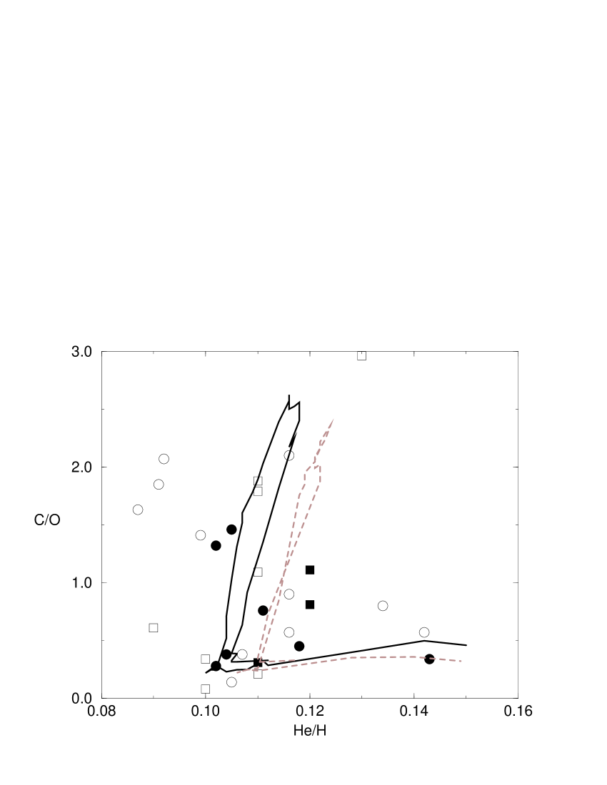
Figure 3: The symbols have the same meaning as figure 2. The dashed line are the [Fe/H]=0.1 models.

2.6 Results

The resulting stellar yields are given in Table 1 for 5 values of metallicities: $\log{(Z/Z_{\odot})}=-0.2$, -0.1, 0.0, +0.1 and +0.2, and for masses from 1 to 8 $M_{\odot}$. We show in Table 1 only the solar metallicity results. The complete table with the other metallicity sets is available in electronic format. These resulting yields for ¹²C, ¹³C, ¹⁴N and ¹⁶O are represented in Fig. 4.

The yield of ${}^{12}{\rm C}$ is shown in panel a of Figure 4. This is approximately zero for the lowest mass stars which exhibit no dredge–up events. As the metallicity is decreased, stars of lower mass will produce carbon because dredge–up events occur in lower mass stars at lower metallicities. The sharp drop–off in the carbon yield occurs when stars get massive enough to exhibit HBB. This produces a negative yield because the carbon in the envelope is converted into nitrogen.

Figure 4: Total yields of ${}^{12}C$, ${}^{13}C$, ${}^{14}N$ and ${}^{16}O$ produced by LIM stars for different metallicities following label in panel d, expressed as $log{(Z/Z_{\odot})}$.

The yield of ${}^{14}{\rm N}$ (Figure 4, panel b has a local maximum at $\sim 3.5--5M_{\odot}$ and then decreases slightly before beginning to increase as a function of stellar mass. Significant amounts of nitrogen are produced solely for intermediate mass stars because HBB and the 2^nd dredge–up occur only in stars with $M>3.5--5M_{\odot}$. The yields at lower masses are due to the 1^st dredge–up.

HBB produces higher luminosities, larger radii and the mass–loss rate increases correspondingly in the stars undergoing this process. As a consequence, stars which experience HBB have shorter TP–AGB lifetimes compared to those that do not experience HBB. This shorter TP–AGB lifetime results in fewer 3^rd dredge–up events and less new carbon mixed into the envelope that can be converted into primary nitrogen. The local maximum between 3.5 and 5 ${{\rm M}_{\odot}}$ is where significant nitrogen production due to HBB begins. Models below the mass of this maximum have lifetimes $\sim 10$ times greater than those above this maximum. The transition occurs at the onset of hot–bottom burning. The amount of material dredged–up decreases by a large factor through this transition zone while the amount of hot–bottom burning increases, producing the local maximum.

The yield of ${}^{13}{\rm C}$ (Figure 4, panel c has a maximum around $\sim 4--5M_{\odot}$, but this element is also produced in a smaller quantity for stars with masses $M>5--6M_{\odot}$. This is mostly a primary component. The yield of oxygen (Figure 4, panel d is negative in all stars.

We will compare these yields with those of other authors in the following section, in particular the proportion of secondary nitrogen produced in each case.

Mass	H	He	C12	N14	O16	C13	C12P	N14P	O16P	C13P
$\rm[Fe/H]=0.0$
1.00	-0.13E-01	0.13E-01	-0.35E-03	0.40E-03	-0.42E-04	0.30E-04	0.00E+00	0.00E+00	0.00E+00	0.00E+00
1.10	-0.14E-01	0.14E-01	-0.42E-03	0.50E-03	-0.51E-04	0.36E-04	0.00E+00	0.00E+00	0.00E+00	0.00E+00
1.20	-0.16E-01	0.16E-01	-0.51E-03	0.59E-03	-0.59E-04	0.42E-04	0.00E+00	0.00E+00	0.00E+00	0.00E+00
1.30	-0.17E-01	0.17E-01	-0.59E-03	0.69E-03	-0.68E-04	0.48E-04	0.00E+00	0.00E+00	0.00E+00	0.00E+00
1.40	-0.17E-01	0.17E-01	-0.67E-03	0.78E-03	-0.76E-04	0.53E-04	0.00E+00	0.00E+00	0.00E+00	0.00E+00
1.50	-0.17E-01	0.17E-01	-0.76E-03	0.89E-03	-0.84E-04	0.58E-04	0.00E+00	0.00E+00	0.00E+00	0.00E+00
1.60	-0.17E-01	0.17E-01	-0.85E-03	0.99E-03	-0.93E-04	0.63E-04	0.00E+00	0.00E+00	0.00E+00	0.00E+00
1.62	-0.17E-01	0.17E-01	-0.87E-03	0.10E-02	-0.94E-04	0.64E-04	0.00E+00	0.00E+00	0.00E+00	0.00E+00
1.64	-0.17E-01	0.17E-01	-0.86E-03	0.10E-02	-0.97E-04	0.65E-04	0.29E-04	0.00E+00	0.14E-06	0.00E+00
1.66	-0.18E-01	0.18E-01	-0.62E-03	0.10E-02	-0.11E-03	0.66E-04	0.29E-03	-0.88E-23	0.14E-05	0.00E+00
1.68	-0.18E-01	0.18E-01	-0.56E-03	0.11E-02	-0.11E-03	0.67E-04	0.36E-03	0.00E+00	0.17E-05	0.00E+00
1.70	-0.19E-01	0.18E-01	-0.21E-03	0.11E-02	-0.13E-03	0.68E-04	0.74E-03	0.29E-21	0.36E-05	0.00E+00
1.80	-0.24E-01	0.22E-01	0.15E-02	0.12E-02	-0.20E-03	0.72E-04	0.26E-02	0.00E+00	0.13E-04	0.00E+00
1.90	-0.32E-01	0.26E-01	0.41E-02	0.13E-02	-0.31E-03	0.76E-04	0.53E-02	0.00E+00	0.27E-04	0.00E+00
2.00	-0.42E-01	0.33E-01	0.79E-02	0.14E-02	-0.46E-03	0.79E-04	0.92E-02	0.00E+00	0.48E-04	0.00E+00
2.10	-0.55E-01	0.41E-01	0.12E-01	0.15E-02	-0.63E-03	0.82E-04	0.14E-01	0.18E-20	0.73E-04	0.00E+00
2.20	-0.69E-01	0.50E-01	0.17E-01	0.15E-02	-0.80E-03	0.84E-04	0.18E-01	-0.81E-18	0.98E-04	0.00E+00
2.30	-0.72E-01	0.52E-01	0.18E-01	0.17E-02	-0.85E-03	0.89E-04	0.19E-01	0.43E-17	0.11E-03	0.00E+00
2.40	-0.81E-01	0.58E-01	0.21E-01	0.18E-02	-0.96E-03	0.92E-04	0.23E-01	0.37E-17	0.13E-03	0.00E+00
2.50	-0.86E-01	0.61E-01	0.22E-01	0.19E-02	-0.10E-02	0.95E-04	0.25E-01	0.90E-18	0.14E-03	0.00E+00
2.60	-0.92E-01	0.65E-01	0.25E-01	0.20E-02	-0.11E-02	0.98E-04	0.27E-01	0.44E-17	0.15E-03	0.00E+00
2.80	-0.97E-01	0.67E-01	0.26E-01	0.23E-02	-0.12E-02	0.11E-03	0.29E-01	-0.70E-17	0.17E-03	0.00E+00
2.90	-0.10E+00	0.69E-01	0.28E-01	0.24E-02	-0.13E-02	0.11E-03	0.30E-01	-0.14E-19	0.18E-03	0.00E+00
3.10	-0.10E+00	0.71E-01	0.30E-01	0.26E-02	-0.14E-02	0.12E-03	0.32E-01	-0.63E-18	0.20E-03	0.00E+00
3.30	-0.11E+00	0.75E-01	0.33E-01	0.28E-02	-0.15E-02	0.12E-03	0.36E-01	0.77E-17	0.23E-03	0.00E+00
3.40	-0.12E+00	0.79E-01	0.35E-01	0.29E-02	-0.15E-02	0.13E-03	0.38E-01	-0.12E-17	0.25E-03	0.00E+00
3.50	-0.12E+00	0.81E-01	0.36E-01	0.30E-02	-0.16E-02	0.13E-03	0.39E-01	0.70E-17	0.26E-03	0.00E+00
3.60	-0.11E+00	0.74E-01	0.33E-01	0.32E-02	-0.15E-02	0.14E-03	0.36E-01	0.28E-17	0.25E-03	0.00E+00
3.70	-0.97E-01	0.64E-01	0.28E-01	0.33E-02	-0.13E-02	0.15E-03	0.31E-01	0.41E-17	0.24E-03	0.00E+00
3.80	-0.89E-01	0.59E-01	0.26E-01	0.34E-02	-0.12E-02	0.15E-03	0.29E-01	0.58E-09	0.25E-03	0.25E-07
3.90	-0.84E-01	0.56E-01	0.24E-01	0.36E-02	-0.12E-02	0.16E-03	0.27E-01	0.12E-06	0.25E-03	0.46E-05
4.00	-0.76E-01	0.51E-01	0.21E-01	0.37E-02	-0.11E-02	0.29E-03	0.25E-01	0.41E-05	0.24E-03	0.10E-03
4.02	-0.70E-01	0.47E-01	0.18E-01	0.40E-02	-0.10E-02	0.15E-02	0.22E-01	0.16E-03	0.22E-03	0.10E-02
4.04	-0.65E-01	0.43E-01	0.12E-01	0.61E-02	-0.97E-03	0.37E-02	0.17E-01	0.18E-02	0.20E-03	0.27E-02
4.06	-0.59E-01	0.39E-01	0.67E-02	0.10E-01	-0.94E-03	0.41E-02	0.13E-01	0.47E-02	0.19E-03	0.27E-02
4.08	-0.54E-01	0.36E-01	0.13E-02	0.16E-01	-0.92E-03	0.31E-02	0.88E-02	0.84E-02	0.17E-03	0.19E-02
4.10	-0.50E-01	0.33E-01	-0.15E-02	0.19E-01	-0.92E-03	0.22E-02	0.67E-02	0.10E-01	0.16E-03	0.12E-02
4.20	-0.37E-01	0.25E-01	-0.69E-02	0.22E-01	-0.13E-02	0.45E-03	0.30E-02	0.11E-01	0.12E-03	0.15E-03
4.30	-0.27E-01	0.18E-01	-0.77E-02	0.20E-01	-0.20E-02	0.32E-03	0.26E-02	0.72E-02	0.94E-04	0.12E-03
4.40	-0.16E-01	0.10E-01	-0.83E-02	0.17E-01	-0.21E-02	0.23E-03	0.22E-02	0.34E-02	0.60E-04	0.85E-04
4.50	-0.30E-01	0.25E-01	-0.85E-02	0.18E-01	-0.26E-02	0.23E-03	0.22E-02	0.32E-02	0.60E-04	0.92E-04
4.60	-0.46E-01	0.41E-01	-0.87E-02	0.19E-01	-0.34E-02	0.24E-03	0.22E-02	0.34E-02	0.63E-04	0.11E-03
4.70	-0.64E-01	0.58E-01	-0.89E-02	0.20E-01	-0.40E-02	0.25E-03	0.22E-02	0.37E-02	0.68E-04	0.12E-03
4.80	-0.81E-01	0.74E-01	-0.91E-02	0.21E-01	-0.46E-02	0.26E-03	0.23E-02	0.40E-02	0.74E-04	0.13E-03
4.90	-0.98E-01	0.91E-01	-0.92E-02	0.22E-01	-0.53E-02	0.27E-03	0.24E-02	0.44E-02	0.80E-04	0.14E-03
5.00	-0.11E+00	0.11E+00	-0.94E-02	0.23E-01	-0.58E-02	0.28E-03	0.24E-02	0.48E-02	0.86E-04	0.15E-03
6.00	-0.28E+00	0.26E+00	-0.11E-01	0.35E-01	-0.13E-01	0.41E-03	0.27E-02	0.87E-02	0.16E-03	0.21E-03
7.00	-0.42E+00	0.41E+00	-0.13E-01	0.42E-01	-0.17E-01	0.48E-03	0.28E-02	0.90E-02	0.19E-03	0.20E-03
8.00	-0.55E+00	0.54E+00	-0.16E-01	0.42E-01	-0.18E-01	0.47E-03	0.24E-02	0.56E-02	0.15E-03	0.14E-03

Table 1: Yields produced in low and intermediate stars for solar metallicity

3 Comparison with other yields

3.1 The set of stellar yields used

Our initial objective is to check the complete set of metallicity-dependent yields for LIM stars (m $<=8\rm M_{\odot}$) obtained as explained in Section 2, using it as the input in a Galactic chemical evolution model. First, we would like to compare the results of the yields presented here with those produced by the use of other standard yields.

To compare our yields, hereafter BU, we have selected VG and MA ones. BU yields are calculated for five metallicities, as described, MA are given for three ($Z=0.004$, 0.008, and 0.02), and the VG yields have the same metallicity values as MA plus $\rm Z=0.001$ and $\rm Z=0.04$. For what refers to RV yields, the most widely used set in this range of mass, since they have been improved by the most recent cited works we will not use them. However we compare in this section our resulting yields with those from RV, too.

Figure 5: Total yields of ${}^{12}C$, ${}^{13}C$, ${}^{14}N$ and ${}^{16}O$ produced by LIM stars of solar composition in this work, called BU, compared with those given by RV, VG, MA, VE and DR marked with different symbols according panel d.

We compare the BU yields corresponding to solar metallicity, with those of other authors in Fig. 5. There we have also included the yields recently computed by Ventura, D’Antona & Mazzitelli (2002), VEN (open dots), and by Dray et al. (2003), DR (stars). Although we will not use these two sets, mostly due to their smaller range of stellar mass and/or Z of the computed models compared with the ours, we want to check that BU yields are not in disagreement with those computed with more precise techniques.

We see in panel a, which refers to ${}^{12}C$, that yields from RV (model with $\alpha=1.50$ and $\eta=0.33$ of their Table 3d) are the largest producer of carbon. Yields from MA (their models for $\alpha=2$) are similar to BU, but, as they are calculated assuming $M_{up}=5M_{\odot}$, that is, only for stellar masses lower than (or equal to) this value, they stop at the mass for which our yields becomes negative. The final effect is a larger total yield for MA compared to BU when the integration is done over the whole LIM stellar range. The values given by VG (their model from Table 17, solar abundance, $\eta_{AGB}=4$ and $m_{HBB}=0.8M_{\odot}$) are lower for stellar masses smaller than 4 $M_{\odot}$, but they remain positive or almost zero after that, while BU yields are negative for the most massive LIM stars. DR also produces a strong maximum around 3 $M_{\odot}$ in ${}^{12}C$, although slightly lower than BU. Unfortunately, VE only give values for stellar masses larger than 3.5$M_{\odot}$ which prevents us from checking if the value of the maximum in BU yields must be decreased, as the DR line seems to suggest. The behavior of VE after 4$M_{\odot}$ is similar to the BU and DR models with negative and decreasing values for increasing stellar masses.

These negative values correspond to the production of nitrogen in the same range of mass, seen in panel b. It is clear that RV yields also produce a larger amount of nitrogen than BU. The differences with RV are due to the time the models undergo HBB. In our models, which achieve higher base temperatures than RV, the HBB epoch lasts approximately one-tenth of their time. Therefore, RV models burn more O into N. On the other hand, MA and VG produce negligible nitrogen yields for solar metallicity in comparison with RV. BU shows an intermediate behavior between these two extremes. The yields from VEN falls on the VG values, while DR has similar yields to both except the last point for 6$M_{\odot}$, which is equal to that of BU. In this case the maximum obtained by BU around 4 $M_{\odot}$ does not appear in any of the two new yields, VEN or DR. We think that it is a problem of sampling, since a smaller step in the computed stellar masses is necessary to see this effect.

For ${}^{13}C$, panel c, differences between authors are small: RV, BU, MA, and even DR show a large maximum around 4-5 $M_{\odot}$, while VG and VEN results are very low without a maximum. Panel d shows yields for oxygen, where it is evident that all of them are negative for $M>4M_{\odot}$, as expected, due to the production of N by the CNO cycle.

We caution about the sampling problem that appears with some yield sets. Due to the wide mass step used in the tables, yields have not always been computed for the mass for which the maximum appears in BU yields. Our models will calculate the corresponding yield by interpolating between these two values but, if a maximum was between them, it would be missed. This implies that the integrated yield along the Initial Mass Function (IMF) might be smaller than the true value. We suggest the use of a smaller step in the range between 3 to 5 $M_{\odot}$ to compute stellar models so as not to lose those phases of the star that are important and in which the largest amounts of elements are ejected.

All these differences will have an effect on the final abundances obtained by the chemical evolution model, as we will see in Section 4. Besides the differences existing between the published stellar yields, we have shown that the BU yields are not in disagreement with more precise techniques used recently. Due to the shorter computation time need to obtain BU yields, these could be calculated for a wide range of stellar masses and Z to see details on the stellar mass dependence, which are not otherwise seen. Therefore, until the new techniques are refined and their corresponding results are available, the BU yields are accredited to be used in chemical evolution models.

3.2 The final input: the ejected masses of elements

We now must add the set of massive stars yields, (m $>8\rm M_{\odot}$) in order to have the whole mass range to include in a chemical evolution galaxy model. We have chosen the yields of WW and PCB for massive stars. The choice of WW is made because it is a well–known set used as a reference by many authors. We have also chosen PCB yields because the treatment they give to the mass loss by winds is accurate and because they use the evolutionary tracks of the Padova Group, that are widely known. We do not need to compute models using more yield sets because they have already been compared in other works. We will refer to these other works in Section 5.

M	Mrem	H	He4	C	13C	N	13Cs	Ns	O
$Z=0.02$
0.80	0.53	1.81E-01	8.30E-02	5.80E-04	0.00E+00	0.00E+00	2.90E-05	4.43E-04	2.04E-03
1.00	0.56	0.30E+00	0.14E+00	0.90E-03	0.00E+00	0.00E+00	0.47E-04	0.77E-03	0.33E-02
1.10	0.57	0.36E+00	0.16E+00	0.11E-02	0.00E+00	0.00E+00	0.56E-04	0.93E-03	0.40E-02
1.20	0.57	0.42E+00	0.19E+00	0.12E-02	0.00E+00	0.00E+00	0.65E-04	0.11E-02	0.47E-02
1.30	0.59	0.49E+00	0.21E+00	0.14E-02	0.00E+00	0.00E+00	0.74E-04	0.13E-02	0.53E-02
1.40	0.60	0.55E+00	0.24E+00	0.16E-02	0.00E+00	0.00E+00	0.82E-04	0.14E-02	0.60E-02
1.50	0.62	0.61E+00	0.26E+00	0.17E-02	0.00E+00	0.00E+00	0.90E-04	0.16E-02	0.66E-02
1.60	0.63	0.67E+00	0.29E+00	0.19E-02	0.00E+00	0.00E+00	0.99E-04	0.18E-02	0.73E-02
1.62	0.63	0.68E+00	0.29E+00	0.19E-02	0.00E+00	0.00E+00	0.10E-03	0.18E-02	0.75E-02
1.64	0.63	0.69E+00	0.29E+00	0.20E-02	0.00E+00	0.00E+00	0.10E-03	0.19E-02	0.76E-02
1.66	0.63	0.71E+00	0.30E+00	0.23E-02	0.00E+00	0.00E-00	0.10E-03	0.19E-02	0.77E-02
1.68	0.63	0.72E+00	0.31E+00	0.24E-02	0.00E+00	0.00E+00	0.11E-03	0.19E-02	0.78E-02
1.70	0.64	0.73E+00	0.31E+00	0.28E-02	0.00E+00	0.29E-21	0.11E-03	0.20E-02	0.79E-02
1.80	0.65	0.79E+00	0.34E+00	0.47E-02	0.00E+00	0.00E+00	0.11E-03	0.21E-02	0.86E-02
1.90	0.65	0.85E+00	0.37E+00	0.76E-02	0.00E+00	0.00E+00	0.12E-03	0.23E-02	0.92E-02
2.00	0.66	0.90E+00	0.40E+00	0.12E-01	0.00E+00	0.00E+00	0.13E-03	0.25E-02	0.97E-02
2.10	0.67	0.96E+00	0.44E+00	0.16E-01	0.00E+00	0.18E-20	0.14E-03	0.26E-02	0.10E-01
2.20	0.68	0.10E+01	0.47E+00	0.21E-01	0.00E+00	0.00E-18	0.14E-03	0.28E-02	0.11E-01
2.30	0.68	0.11E+01	0.50E+00	0.22E-01	0.00E+00	0.43E-17	0.15E-03	0.30E-02	0.11E-01
2.40	0.69	0.11E+01	0.53E+00	0.25E-01	0.00E+00	0.37E-17	0.15E-03	0.32E-02	0.12E-01
2.50	0.70	0.12E+01	0.56E+00	0.28E-01	0.00E+00	0.90E-18	0.16E-03	0.34E-02	0.13E-01
2.60	0.71	0.12E+01	0.58E+00	0.30E-01	0.00E+00	0.44E-17	0.17E-03	0.35E-02	0.13E-01
2.80	0.73	0.14E+01	0.64E+00	0.32E-01	0.00E+00	0.00E-17	0.18E-03	0.40E-02	0.15E-01
2.90	0.73	0.14E+01	0.66E+00	0.34E-01	0.00E+00	0.00E-19	0.19E-03	0.42E-02	0.15E-01
3.10	0.75	0.16E+01	0.72E+00	0.36E-01	0.00E+00	0.00E-18	0.20E-03	0.46E-02	0.16E-01
3.30	0.77	0.17E+01	0.77E+00	0.40E-01	0.00E+00	0.77E-17	0.22E-03	0.49E-02	0.18E-01
3.40	0.78	0.17E+01	0.80E+00	0.42E-01	0.00E+00	0.00E-17	0.22E-03	0.51E-02	0.18E-01
3.50	0.79	0.18E+01	0.83E+00	0.43E-01	0.00E+00	0.70E-17	0.23E-03	0.53E-02	0.19E-01
3.60	0.81	0.19E+01	0.84E+00	0.40E-01	0.00E+00	0.28E-17	0.24E-03	0.55E-02	0.20E-01
3.70	0.82	0.19E+01	0.86E+00	0.36E-01	0.00E+00	0.41E-17	0.25E-03	0.57E-02	0.21E-01
3.80	0.84	0.20E+01	0.87E+00	0.34E-01	0.25E-07	0.58E-09	0.26E-03	0.59E-02	0.21E-01
3.90	0.87	0.21E+01	0.89E+00	0.32E-01	0.46E-05	0.12E-06	0.27E-03	0.60E-02	0.22E-01
4.00	0.89	0.21E+01	0.91E+00	0.30E-01	0.10E-03	0.41E-05	0.30E-03	0.62E-02	0.23E-01
4.02	0.88	0.21E+01	0.91E+00	0.27E-01	0.10E-02	0.16E-03	0.59E-03	0.64E-02	0.23E-01
4.04	0.87	0.22E+01	0.92E+00	0.21E-01	0.27E-02	0.18E-02	0.12E-02	0.70E-02	0.23E-01
4.06	0.86	0.22E+01	0.92E+00	0.16E-01	0.27E-02	0.47E-02	0.14E-02	0.81E-02	0.23E-01
4.08	0.86	0.22E+01	0.92E+00	0.10E-01	0.19E-02	0.84E-02	0.13E-02	0.99E-02	0.24E-01
4.10	0.85	0.22E+01	0.93E+00	0.75E-02	0.12E-02	0.10E-01	0.11E-02	0.11E-01	0.24E-01
4.20	0.86	0.23E+01	0.94E+00	0.25E-02	0.15E-03	0.11E-01	0.42E-03	0.14E-01	0.24E-01
4.30	0.87	0.24E+01	0.96E+00	0.19E-02	0.12E-03	0.72E-02	0.33E-03	0.16E-01	0.24E-01
4.40	0.89	0.25E+01	0.98E+00	0.15E-02	0.85E-04	0.34E-02	0.27E-03	0.16E-01	0.25E-01
4.50	0.90	0.25E+01	0.10E+01	0.16E-02	0.92E-04	0.32E-02	0.27E-03	0.17E-01	0.25E-01
4.60	0.91	0.26E+01	0.11E+01	0.16E-02	0.11E-03	0.34E-02	0.26E-03	0.18E-01	0.25E-01
4.70	0.91	0.26E+01	0.11E+01	0.17E-02	0.12E-03	0.37E-02	0.27E-03	0.19E-01	0.25E-01
4.80	0.92	0.27E+01	0.11E+01	0.18E-02	0.13E-03	0.40E-02	0.27E-03	0.20E-01	0.25E-01
4.90	0.93	0.27E+01	0.12E+01	0.19E-02	0.14E-03	0.44E-02	0.28E-03	0.21E-01	0.25E-01
5.00	0.93	0.28E+01	0.12E+01	0.20E-02	0.15E-03	0.48E-02	0.28E-03	0.22E-01	0.25E-01
6.00	0.99	0.33E+01	0.16E+01	0.28E-02	0.21E-03	0.87E-02	0.39E-03	0.31E-01	0.25E-01
7.00	1.04	0.38E+01	0.20E+01	0.35E-02	0.20E-03	0.90E-02	0.50E-03	0.38E-01	0.29E-01
8.00	1.08	0.43E+01	0.24E+01	0.38E-02	0.14E-03	0.56E-02	0.60E-03	0.42E-01	0.34E-01

Table 2: Ejected mass by the LIM stars during their evolution. We only present results for LIM stars, solar metallicity and elements until oxygen. The complete table with the whole range in mass and metallicity is only available in electronic format.

Thus, for massive stars we will use WW and PCB while we have used three set of yields for LIM stars: those presented here, VG and MA. We have combined them, obtaining 3 models: 1) BU-WW; 2) VG-WW; 3) MA-PCB, which we call BU, VG and MA.

Some authors produce yields while others give their results as ejections, which are not equivalent. The stellar yield of an element is the amount that has been newly created and ejected during the evolution of the star, while the ejection computes not only this new mass of the element but the original one, which corresponds to the initial metallicity of the star, too. The yield can be negative, if the star transforms more of the element than it creates, but the ejection is always positive. The formula to transform one into the other (Tinsley, 1980) is:

$$E_{i}=Y_{i}+(M_{ini}-M_{rem})X_{i}$$ (12)

where $E_{i}$ is the ejected mass of the element i, $Y_{i}$ is the value of the yield for the same element, $M_{ini}$ is the initial mass of the star, $M_{rem}$ is the remnant mass and $X_{i}$ is the original stellar abundance of the i-element.

The different ways of presenting the data should be taken into account when the input values of the model for the whole mass range are constructed. WW and PCB give their results as ejected masses for each element while RV, MA and BU directly produce the stellar yields, so we have to transform all them into the same type of quantity before using them as code inputs. We follow the formalism of PCB for the matrix elements $Q_{i,j}$, as we describe in the next section, so we prefer to work with ejections, in order to directly apply their equations. In the present work, we have included both the stellar yields in Table 1, already described, and the corresponding ejections in Table 2.

Thus, we show in this last table the complete ejected mass set for some metallicities. The mass ejected for each element is given by each stellar mass from $m_{low}=0.8M_{\odot}$ to $m_{sep}=8M_{\odot}$ for solar metallicity. Column (1) is the stellar mass, column (2) is the remnant mass, columns (3) to (10) show the ejected mass of ${}^{12}C$, ${}^{13}C$, ${}^{14}N$, ${}^{16}O$, and ${}^{12}C_{P}$, ${}^{13}C_{P}$, ${}^{14}N_{P}$, ${}^{16}O_{P}$. These values result from the computed yields shown in Table 1. The complete table, given only in electronic format, provides results for metallicities $log(Z/{{\rm Z}_{\odot}})=-0.2$,-0.1,+0.0,+0.1 and +0.2, by including the massive star yields, for masses up to $m_{up}=100M_{\odot}$. This implies that columns (3) to (10) correspond to CNO elements, as explained, but columns from (11) to (16) show the ejected masses for other elements produced only by massive stars: Ne, Mg, Si, S, Ca and Fe. For massive stars these quantities are obtained from the production factors by WW. A similar table has been computed for the two other models, VG and MA.

In all cases we use metallicity–dependent yields. However, the range of metallicity for which the yields are given is different for each set. It has been necessary to transform them into homogeneous and consistent sets for which we have adapted the values of the metallicity of massive and LIM stars to a common set in each model. When the metallicities are not the same for the massive star set as for the LIM star yields, as occurs with models BU and VG with respect to WW, we need to interpolate in Z to obtain a complete table for each Z. In that case, we have preferred to interpolate the massive star yields to compute them at the metallicities given for LIM stars, because they have a more continuous variation in Z for the whole mass range than LIM stars. Thus, for instance, for BU we have the yields for $Z=0.0159$, and we interpolate those from WW between $Z=0.1Z_{\odot}$ and $Z=Z_{\odot}$ at this same abundance value. We use the same technique for the two other sub–solar metallicities (-0.2,-0.5), by interpolating between tables corresponding to $Z=Z_{\odot}$ and Z=0.1Z_⊙. For the over–solar sets, and because that WW do not give yields for metal–rich stars, we have extrapolated their solar yields to use with the yields of $Z=0.025$ and $Z=0.0317$ from BU. For the VG model we also interpolate in the massive stars tables to obtain the complete tables at the abundances given by VG, from $Z=0.001$ to $Z=0.04$.

When we use MA with PCB yields the problem is smaller because both sets are calculated for a similar set of abundances. However, MA do not give results for the lowest abundances in the Padova group, $Z=0.0004$. We have analyzed if the trend in Z is clear and continuous, and as this does not occur for ${}^{14}N$, as we will see later, we have preferred to use the smallest metallicity yields from MA ($Z=0.004$) along with tables for $Z=0.0004$ from PCB.

4 Galactic Chemical Evolution Models

4.1 Summary description of the multiphase chemical evolution model

The model used in this work is the Multiphase Chemical Evolution Model described in Ferrini et al. (1992, 1994), in the version presented in Mollá & Díaz (2004). The Galaxy is considered as a two–zone system: halo and disk, sliced into cylindrical concentric regions. It calculates the time evolution of five different populations or matter phases in the Milky Way: diffuse gas, molecular clouds, low and intermediate stars, massive stars and stellar remnants.

The corresponding yields for type Ia and Ib supernova explosions, included in calculations following Tornambé (1989) and Ferrini & Poggiantti (1993), are taken from Iwamoto et al. (1999) and Branch & Nomoto (1986). The assumed initial mass function is from Ferrini, Penco & Palla (1990), very similar to the one given by Kroupa (2001).

The chemical abundances of 15 elements are computed through the Q–matrix technique. The Q–matrix is based on the Talbot & Arnett (1973) formalism and well described in previous publications of this code. Each element of the matrix, $Q_{i,j}$ is the mass fraction of the star initially in the form of species $j$ that has been transformed to species $i$ and ejected. The original formalism changes for the metallicity–dependent yields. Thus, we have taken the equations given by PCB for all elements except for D and ${}^{3}He$, for which the relations given by Galli et al. (1995) are used. To compute the Q–matrix we use the tables with the ejected masses of elements computed as described in the previous section.

4.2 Calibration: The solar neighborhood

Figure 6: Time evolution in the Solar Vicinity: a) the star formation history and b) the age–metallicity relation. Data are from Twarog (1980) (TWA), Barry (1988) (BA), Edvardsson et al. (1993) (EDV), Carraro, Ng & Portinari (1998) (CAR), Rocha-Pinto et al. (2000a, b) (RO) and Reddy et al. (2003).

We now use the three described sets of yields in the GCE Model. The model was already used in the Solar Vicinity (SV), assumed as the region located at a galactocentric distance of 8 kpc, and in the Galactic disk, (Ferrini et al., 1992, 1994), so we do not need to again compare atomic and molecular gas, or star formation rate radial distributions with data ( but see Mollá & Díaz, 2004, for a revised comparison of these observational constraints with the model).

However, as we are using a new version of the code where metallicity–dependent yields have been implemented, we have to check that model results are still correct. On the other hand, as our objective is to compare the resulting carbon abundances given by different stellar yields, only other relations where these element yields have no influence must be analyzed. Thus, in this section we only use model results independent of the selected yield set. So, we choose the SFR history, the age–metallicity relation and the G–dwarf metallicity distribution, all of them for the Solar Vicinity, a well–known region where the number of observational constraints is high.

In Fig. 6 we have: a) the star formation history and b) the age–metallicity relation for the SV. Our 3 models, BU, VG, and MA, are represented by solid, short–dashed, and dotted lines respectively. The star formation history recently obtained by Rocha-Pinto et al. (2000b) shows a behavior more similar to the one obtained from hydrodynamical simulations of galaxy formation (Sáiz, Domínguez-Tenreiro & Serna, 2003), with strong variations with the time compared to the smoother line from the Twarog (1980) data. Nevertheless, the average star formation history is similar, with a maximum around 3 Gyr and another, more recent, around 10 Gyr.

The age–metallicity relation, which mostly depends on SN–I iron ejection, is almost the same for all models. Some differences are apparent however, because a quantity of iron is also ejected by massive stars. The PCB yields produce more iron t iron than those from WW, and therefore model MA shows a higher metallicity at early times than models BU and VG. In order to better reproduce the present abundance data, the rate of SN–Ia was decreased in model MA, compared to WW. Due to this the iron will appear later in WW models than in the model MA. This will have an effect on our final results.

Figure 7: G–dwarf distribution for our model compared with data from Chang, Hou & Fu (2000); Kotoneva et al. (2002) in a) and with data from Jørgensen (2000) in b).

The G–dwarf metallicity distribution is shown in Fig. 7 for our model BU and compared with data from Jørgensen (2000). We see that the model produces iron with a maximum around -0.10 dex, very similar to the observed average which is $\sim 0.16$ dex. This distribution is much more peaked (or less wide) than those found in others works (Pagel, 1989; Chang, Hou & Fu, 2000; Rocha-Pinto et al., 2000a) and similar to the one from Kotoneva et al. (2002). These last authors confirm that the solar vicinity formed over a long time scale, of the order of 7 Gyr, similar to ours. Taking into account the dispersion of measurements, estimated by the variations shown by these different sets of data, the modeled distribution may be considered acceptable. Since iron comes mostly from SN–Ia, the resulting distribution for the model MA is similar which for the sake of clarity we do not show.

Once a suitable calibration of the model is obtained, we can analyze the differences of carbon abundances resulting from the cited sets of yields.

4.3 The time evolution of CNO abundances

Data used for the comparison in the next figures are taken following Table 3. We start with the time evolution in the Solar Neighborhood.

Fig. 8 shows the evolution of oxygen –panel a– carbon –panel b– and the relative abundance log(C/O) –panel c–. Models are represented by the same symbols as in Fig. 6. There are almost no differences between models for oxygen, all of them being in agreement with the data. Since oxygen proceeds mostly from massive stars, it is obvious than models BU and VG produce equal abundances. Model MA gives a slightly higher abundance (O/H) that corresponds to a larger yield in PCB than in WW.

[Fe/H]	[C/H]	[O/H]	R	Age	Reference
X	X	X	—	—	Akerman et al. (2004)
X	—	X	—	—	Barbuy (1988)
X	—	X	—	—	Barbuy & Erdelyi-Mendes (1989)
X	—	X	—	—	Boesgaard et al. (1999)
X	X	—	—	—	Carbon et al. (1987)
X	X	X	—	—	Carretta, Gratton & Sneden (2000)
X	—	X	—	—	Cavallo, Pilachowski & Rebolo (1997)
X	—	X	—	X	Chen et al. (2000)
X	X	X	—	—	Clegg, Tomkin & Lambert (1981)
X	X	X	—	—	Daflon et al. (2001)
X	X	X	—	—	Depagne et al. (2002)
X	—	X	X	X	Edvardsson et al. (1993)
—	X	—	X	X	Gustafsson et al. (1999)
X	X	—	—	—	Friel & Boesgaard (1990)
X	X	X	—	—	Gratton et al. (2000)
—	X	X	X	—	Gummersbach et al. (1998)
X	—	X	—	—	Israelian, García López & Rebolo (1998)
					Israelian et al. (2001)
X	X	—	—	—	Laird (1985)
X	X	—	—	—	Meléndez & Barbuy (2001)
					Meléndez & Barbuy (2002)
X	—	X	—	—	Mishenina et al. (2000)
X	—	X	—	—	Nissen (2002)
					Nissen et al. (2002)
X	X	—	—	X	Reddy et al. (2003)
X	X	X	X	—	Rolleston et al. (2000)
					Smartt & Rolleston (1997)
					Smartt et al. (2001)
X	X	—	—	—	Shi, Zhao & Chen (2002)
X	—	X	—	—	Smith, Pereira & Cunha (2001)
X	X	X	—	—	Tomkin & Lambert (1984)
					Tomkin, Sneden & Lambert (1986)
					Tomkin (1995)
X	X	X	—	—	Westin et al. (2000)

Table 3: References for CNO stellar abundances used for the comparison with model results.

Figure 8: Time evolution of abundances in the Solar Vicinity: a) oxygen, b) carbon, as $12+log(X/H)$ and c) the ratio C/O. Solar abundances are the filled symbols from Grevesse & Sauval (1998) – circles–, Holweger (2001) –squares– and Allende Prieto, Lambert & Asplund (2001); Allende Prieto et al. (2001); Allende Prieto, Lambert & Asplund (2002), –crosses–, by assuming an age of 4.5 Gyr for the sun. Empty symbols at 13.2 Gyr are the interstellar medium abundances given by Meyer, Cardelli & Sofia (1997); Meyer, Jura & Cardelli (1998), –circles–, Peimbert (1999) –squares–, Sofia et al. (2001), –triangles–, and Moos et al. (2002), –stars. Small open dots are stellar abundances obtained from Table 3, being those located around the Solar Vicinity ($7<R<9$ kpc). Line meanings are given in panel b of Fig. 6.

Differences among models in the carbon abundances are larger than the error bars for the Solar and ISM data: Model BU is located in the lower part of the error bars, while the MA model is above the data. VG shows the lowest values. WW yields do not produce as much carbon as PCB, because the stellar winds, which mostly ejected this element, are not considered in WW. Due to this, MA is the highest in panel b. Models BU and VG are coincident in the first Gyr, when carbon proceeds from the same massive stars. After a time $\sim$ 1.5 Gyr, a difference appears between these two models, indicating a greater carbon production by the BU yields. The final consequence is a better fit of the observations by the model BU.

Similar information can also be extracted from the relative abundances vs time in Fig. 8. The fact that carbon is fit well by the BU–WW yields, without needing massive star yields incorporating mass loss and its dependence on metallicity, probably indicates that the mass loss assumed in massive star yields different to WW is too high.

Several zones are clearly distinguished in panel a as in panel b: first, an abrupt increase which corresponds to the massive star contribution. Afterwards, an almost constant value indicates the region where the bulk of stars between 4 to 8 $M_{\odot}$, which do not eject carbon, are dying. Then, intermediate mass stars ($M\sim 3-5M_{\odot}$) begin to eject carbon, producing an amount sufficient to reach the present value. This can be seen clearly in this figure, because the point where the models begin to separate is where the LIM stars carbon contribution appears. Carigi (2000) points out that the time evolution shown by this graph seems to indicate an increase of the carbon abundance at recent times and that metallicity–dependent yields are necessary to explain this finding. However, we see that the data may be reproduced by an almost constant evolution of C/O after the increase shown between $\sim$1 and 3 Gyr. An increase for the youngest objects ($\rm t>10$ Gyr) is not apparent. The number of observations has increased and we think that probably the difference in conclusions is due to these more recent stellar data.

4.4 Radial gradients of abundances

Up to now we have only analyzed SV data, but we want to extend the results to the entire disk. We plot the radial gradient of oxygen and carbon as can be seen in Fig. 9. The Hii regions data authors are given in the graph while star data are from Table 3.

Figure 9: Radial distributions of elemental abundances, as 12 + log (X/H), in the Galaxy disk for: a) oxygen, b) carbon and the relative abundance log(C/O). Stellar data –filled dots– are taken from authors given in Table 3. Hii regions abundances are also included, taken from Peimbert (1979) –PE–, Shaver et al. (1983) –SHA–, Fich & Silkey (1991) –FS–, Vílchez & Esteban (1996) –VIES–, Afflerbach, Churchwell & Werner (1997)–AFF-, and Esteban et al. (1999); Esteban, Peimbert & Torres-Peimbert (1999b); Esteban et al. (1999c) –EST– as marked in the figure.

These radial distributions show a correct shape in the three panels. This occurs because the shape depends mostly on the infall/SFR ratio along the galactocentric radius, and it is not yield–dependent. The value of the gradient at the center and at the outer regions is currently a matter of discussion (Vílchez & Esteban, 1996).

We see in panel a that average abundances of oxygen are even in the inner disk, where the distribution flattens. The three model radial distributions lie between the error bars defined by the dispersion of data. In panel b, we show the same kind of graph for the carbon abundance, as $\rm 12+log(C/H)$. As we would expect, the MA model presents higher values than two others and does not reproduce the observations. The two other models fit the data reasonably well.

In panel c of the same figure the relative abundance C/O radial distribution is plotted. In agreement with previous comments, the MA model presents a carbon excess, so it is located outside the data region. We note that the observed C/O radial distribution, after including data from Smartt et al. (2001) and Reddy et al. (2003), does not show a negative slope, as Carigi (2000) suggested.

4.5 The relative abundances of carbon

The relative abundance of an element gives important clues about how the evolution is taking place. In this kind of figure, model parameters like infall rate and star formation efficiency have a smaller influence than in others.

Fig. 10 plots the relation between C/O for the SV region compared with stellar and Hii region data. As we are showing the SV results it would be adequate to compare them with data of the same region but unfortunately some data could belong to other radial regions. The ones from Smartt et al. (2001) correspond to the inner disk, and other sets (Edvardsson et al., 1993; Clegg, Tomkin & Lambert, 1981; Gummersbach et al., 1998) may include stars at different galactocentric distances than the assumed one for the SV. This may partially be the reason for the large data dispersion usually seen in this kind of figure. We try to select data for stars or Hii regions located in the Solar Neighborhood, that is 7 kpc $\rm\leq R\leq$ 9 kpc, in order to decrease the dispersion, but the galactocentric distance is not always given in the sets of data.

We are showing the results representing the evolution of the disk, not that of the halo. In our scenario, both regions are followed separately, and, as the halo regions have very low star formation efficiencies, their evolution is not similar to that in the disk regions. In order to compare with observations, we must choose only disk data. Usually, all low metallicity objects are considered halo objects, but this is not always true. To properly select data, some kinematic information for the stars is necessary. We will use all possible stellar data although some may come from halo stars.

Following the same argument, observations from other galaxies are not adequate too, since their evolution may follow other tracks, because the star formation or infall rate histories are not necessarily equal to the SV region (Mollá, Ferrini & Díaz, 1996; Mollá et al., 1999). As differences in this kind of figure are mainly due to yields, not to the model parameters, and due to the paucity of carbon data in the solar neighborhood, we will use data from other parts of the disk, or even from the halo.

Figure 10: The relative abundances of log (C/O) vs the oxygen abundance as $12+log(O/H)$. Stellar data –open circles– are from Table 3. Other data are from Esteban et al. (1999) –EST99–, Tsamis et al. (2003)–TSA–, for galactic Hii regions, from Garnett et al. (1995, 1999) –GR95/99–, for other galaxies Hii regions and from Izotov & Thuan (1999) –IZ– for Blue compact dwarf galaxies. The meaning of symbols is given in the figure.

The initial value of log (C/O) between -0.7 and -0.8 dex is caused by the evolution of massive stars in the first Myr. The flat left part of the graph must be interpreted having in mind that it takes place in a very short time: the time needed for stars with masses between 5 and 8 $M_{\odot}$ to evolve. Stars in this range do not eject carbon, so the carbon abundance level remains at the level due to the massive stars ejection, whose contribution appears before. When stars with masses close to 4 $M_{\odot}$ begin to die, the carbon increases rapidly and finally reaches a plateau, when the smallest stars evolve without ejecting CNO cycle elements.

This interpretation is valid for all models, and to clearly show our argument crosses have been marked on the model lines to indicate the times corresponding to 0.25, 0.50, 0.75, 1.0, 1.5 and 2 Gyr since time zero of the galaxy evolution. The model predicts a continuous star formation history with a maximum at $\sim 1.8$ Gyr. Most of stars create in this period and more massive than 4 $M_{\odot}$) (whose lifetime is $\tau=0.165$ Gyr) no longer exist at $t=2$ Gyr.

The BU model reaches final values closer to the observations. The MA model gives a final log(C/O) slightly higher, due to the large production of carbon in PCB for massive stars. This production is caused by the high mass loss assumed for the stellar winds, and the comparison between model and data may imply that the assumed mass loss is too strong.

Now, we will analyze the abundances vs the iron abundances. Once again we cannot separate disk and halo objects, so we consider that disk objects are those with [Fe/H] greater than -1.5. This method is not as useful for discriminating between halo and disk stars as the use of kinematic information, and some halo stars will be included while some other disk objects of low metal content will be missed.

Figure 11: The relative abundances of C and O as [X/Fe] vs the iron abundance [Fe/H]. Panel a shows the [O/Fe] evolution for the disk. The dot–long– dashed line represents the trend of Boesgaard et al. (1999) data. Panels b and c represent the evolution of [C/Fe] for the disk and the halo, respectively. Models have the same line coding as previous figures. Data are taken from authors from Table 3. Open dots are the available data, while solid dots are stars that have known galactocentric distance in the range $7\leq R\leq 9$ kpc. Triangles are data from Carbon et al. (1987).

The following graph depends not only on the carbon ejection but also on the iron production. The iron appears mostly as consequence of the SN–I explosions, which eject a large quantity of this element in each event. However, massive stars also produce Fe and differences among the various stellar yields for these stars have an effect on the results. PCB produce more Fe than WW, and, correspondingly, [X/Fe] will be smaller for PCB yields when the abundances are low, while Fe proceeds from massive stars, independently of the yields used for LIM stars. When the SN–I start to explode, the iron appears in the ISM and [X/Fe] begins to decrease. In order to obtain the same iron at the present time, the SN–Ia rate for the model MA is smaller than the one from models using WW. But this only will be seen at later times. For the early times, the differences may be as high as +0.3 dex in the abundance of [Fe/H].

The usual correlation between [O/Fe] and [Fe/H] is shown in Fig. 11a. Two different trends are usually obtained depending on the technique used to estimate the stellar abundances. The dot–long–dashed line represents the trend given by Boesgaard et al. (1999), steeper than the second one which shows a flatter shape with metallicity for $\rm[Fe/H]<-1$. Actually, if the complete set of data is plotted, the two trends are indistinguishable, as we can see in panel a, although with a large dispersion. Models BU and VG are in agreement with these observations while model MA shows a flatter behaviour at low metallicity.

We represent the relative abundance [C/Fe] vs [Fe/H] for the disk, panel b, and for the halo, panel c, in the same figure. We have used the classical data for [C/Fe], but we remind the reader of our previous argument about the halo and disk as separate entities with different time evolutions. Some data increase with decreasing metallicity, and others seem located at a lower level, around $\rm[C/Fe]\sim\leavevmode\nobreak\ 0$.

We see in panel b that models BU and VG start with a similar evolution as it corresponds to the same set of massive stars yields used. For the disk, both first decrease when metallicity increases. Then, when the contribution of stars with $M\sim 4M_{\odot}$ begins to appear, the BU model increases and has a bump, like the observed one. In fact, it is difficult to see the model line over the data. Finally, it decreases when the lowest mass stars begin to die without ejecting any elements. This model reproduces well the trend described by open dots at $[Fe/H]\geq-1$ (and also the data from Carbon et al., 1987). Model VG, however, continues to decrease after this metallicity, in disagreement with disk data. Model MA produces more iron than the two other models early on, so the absolute [C/Fe] level is lower, than the two other models, around -0.1 dex, until $\rm[Fe/H]=-1$. However it produces too much carbon for $[Fe/H]>-1$. Due to the large dispersion of data, it is difficult to determine which model (BU or VG) better fits the observations, but we think that the BU model is more adequate to fit the disk observations.

The data at low metallicity seem to show two trends shown by open bullets, and by open triangles, which are the observations by Carbon et al. (1987). We suggest that the sets represent the evolution of the halo and the disk, respectively, which are not equivalent. We show the evolution of the halo in panel c for the three models. In this figure there are no lines above $[Fe/H]>-1$ as expected for the halo. It is clear that MA does not reproduce the low metallicity observations. Models BU and VG give results falling in the regions of these data. In particular, in this low metallicity region, the halo of model BU fits well the open dot data while the disk evolution is closer to the triangles

Therefore, we think that these two different trends correspond to the different star formation histories occurring in the halo and in the disk. The BU models are the only ones able to predict the two observed trends in these data sets.

5 Discussion

We have presented new LIM yields and we have used Galaxy chemical evolution models to compare the results with data and with results obtained with other sets of yields. When carbon abundance data are analyzed in a graph of log(C/O) vs (O/H) an almost flat slope appears and then they show an increase until the solar value. This is usually interpreted as the carbon being ejected mostly by massive stars, thus producing a constant proportion of C/O. However, the final abrupt increase of the carbon abundances with increasing oxygen abundance is unexplained.

Carigi (2000) invokes the metallicity dependent yields, due to its effect on mass loss by stellar winds, as essential for solving this problem of obtaining an increase in the ratio C/O in recent times. The effect of the winds, which change with Z, included in the Maeder yields would be able to produce the recent increase. But the relation (C/O) vs (O/H) is not reproduced by any model (see Carigi (2000) Fig.5), in particular the variable slope of log(C/O) with increasing O/H, because the model produces C/O higher than data for the low metallicity region.

Henry, Edmunds & Köppen (2000) also assume that carbon must proceed mostly from massive stars and use Maeder yields, but however, had to adjust the carbon yields by multiplying them by a factor of 3 in order to achieve a good fit to solar data. This seems to be in contradiction to the hypothesis that stellar winds proceeding from massive stars explain this increase. CHIA03, using yields from Thielemann, Nomoto & Hashimoto (1996), also multiply the carbon yields by a factor of 3 so as to reproduce the present time C abundance. Thus, it seems impossible to reproduce the observed trend only with the contribution of massive stars. Therefore, the best yields to reproduce carbon abundances seem to be those from WW. When those authors used WW yields with those from VG, they obtained a result for the C/O very similar to the one from our VG model.

On the other hand, when the most recent data from carbon abundance are used, the increasing trend in the abundance of carbon at recent times, an important argument in Carigi (2000) conclusions, seems to disappear, showing only a large dispersion around a mean C/O mostly flat for $t>3$ Gyr. So, the increase of carbon with respect to the first base level did not occur in the last 2–3 Gyr but much before.

C/O begins to increase when the oxygen abundance is $12+log(O/H)\sim 8.2$, but this does not necessarily mean that it has occured recently. In our models this value is reached at around 1.2 Gyr or more than 10 Gyr ago. Then, when $12+log(C/H)\sim 7.4$, the stars of $\sim 4M_{\odot}$ begin to contribute to the carbon, which is clear in Fig.8b, when models BU and VG, with the same massive star yields, start to separate. The LIM stars which eject carbon have masses between 3 and 5 M_⊙, and have lifetimes around 0.15–0.4 Gyr, short enough in the evolution of the Galaxy. Therefore, the increase of carbon seen in the relation C/O vs O/H is due to the low mass star ejections. It starts to occur between 1.2 and 3.5 Gyr, or, equivalently, 10 to 12 Gyr ago. CHIA03 claim, on the basis of their model results, that a large amount of carbon must originate in LIM stars. Our results are in agreement with this statement. However, the increase of C/O with metallicity is better reproduced when the new set of yields BU is used in combination with that of WW for massive stars. The yields presented here produce results in excellent agreement with data.

Thus, we agree with the conclusion from CHIA03 that the evolution of LIM stars with massive stars without stellar winds may account for the carbon evolution: the contribution of LIM stars to the final abundance of carbon may be sufficient to reproduce the observations. The C ejected by stars with masses around 4 $M_{\odot}$ produces a strong and steep increase in the high abundance region starting around 12+log(O/H)$\sim 8.2$. The resulting curve reproduces the observed trend, in a way not produced by other models.

[C/Fe], instead of C/O, may be analyzed with chemical evolution models. In Liang, Zhao & Shi (2001), who also compare the effect of using several combinations of yields, all figures refer to Fe and not to O. Our model MA has results similar to those shown by Liang, Zhao & Shi (2001) (model MA + PCB) and also by PCB, although the LIM star yields are slightly different (they use Marigo, Bressan & Chiosi, 1996, instead of MA) in this last model. All of them produce a value of [C/Fe] almost constant up to $\rm[Fe/H]=-0.5$ that then increases reaching values higher than observations at the solar metallicity end.

Similarly, CHIA03 also show their results as [C/Fe] vs [Fe/H]. These authors, like Liang, Zhao & Shi (2001) find a very flat behavior in this graph with a slight increase at the high abundance end, that the authors interpret as caused by a significant amount of carbon being ejected by LIM stars. Both works show that Model VG is the best one at reproducing the data corresponding to carbon. Nevertheless, Liang, Zhao & Shi (2001) explained that it is possible to fit the carbon data only with the LIM stars and with stars of $\rm M<40M_{\odot}$, without needing carbon ejected by Wolf–Rayet stars. Our models BU and VG reproduce a very similar trend although BU better fits the data for the high metallicity region, as we see in Fig. 10 and Fig. 11, due to its larger integrated carbon yield.

Since we do not need to invoke a massive star stellar wind effect to reproduce the observed trend in the C/O or C/Fe data, we think that the mass loss for massive stars assumed in works such as Maeder (1992) or PCB is too strong. We are in agreement with Liang, Zhao & Shi (2001) supporting a mass loss lower than assumed in previous works, in the same line as Crowther (2001) who points out that the recent mass–loss rates for Galactic W–R stars indicate a downward revision of a factor of 2–4 compared with the previous calibrations.

We also support the claim of those authors that the ${}^{12}C(\alpha,\gamma)^{16}O$ rate used by WW seems to be adequate. Hashimoto (1995) use the rate from Caughlan et al. (1985)(CFHZ85), a factor $\sim$ 2.4 higher than the most recent rate from Caughlan & Fowler (1988) (CF88), thus producing less carbon. Hashimoto (1995) gives a discussion about this rate, indicating that the rate of CF88 is clearly too low, and produces too much carbon. He claims that, actually, the rate of CFHZ85, a factor 2.4 larger than that of CF88, is more consistent with observations, although they stated that an intermediate value, such as 1.7 times the value of CF88, the one used by Woosley & Weaver (1995), is probably better for this reaction rate.

Thus, although VG yields produce reasonable results, BU yields, with higher absolute values for carbon yields, and following the same trends as VG, better predicts carbon abundances.

6 Conclusions

1. We can reproduce the carbon abundances and the trend of C/O over O/H, in particular its increase at almost solar oxygen abundances, by the effect of LIM stars, without invoking the metallicity dependence (proceeding the stellar mass loss) of carbon yields. This conclusion is in agreement with Liang, Zhao & Shi (2001); Chiappini, Romano & Matteucci (2003), and Chiappini, Matteucci & Meynet (2003). The difference to these last works is that BU yields shown here, with a larger production of carbon than VG, seem to better fit the data of this element.

2. The previous conclusion implies that the mass loss by stellar winds in massive stars probably needs to be smoother than usually assumed. In this sense, we support to Liang, Zhao & Shi (2001) (Meynet & Maeder, 2002, but see) who also claim that the mass loss must be revised downward.

3. The reaction rate for ${}^{12}C(\alpha,\gamma)^{16}O$ taken as 1.7 times the value of CF88 by WW produces results consistent with the observations.

4. The data [C/Fe] for $\rm[Fe/H]>-1.0$ is well reproduced by the evolution of the disk of the BU model. For low metallicities, the observations may be divided into two trends. One of them is well reproduced by our disk model results, while the second one is well fitted by the same BU model with the halo results. These conclusions are in agreement with recent results from Chiappini, Romano & Matteucci (2003), who also show that the halo and the disk have different evolutions.