ASCA Compilation of X-Ray Properties of Hot Gas in Elliptical Galaxies and Galaxy Clusters: Two Breaks in the Temperature Dependences

Abstract

Utilizing ASCA archival data of about 300 objects of elliptical galaxies, groups, and clusters of galaxies, we performed systematic measurements of the X-ray properties of hot gas in their systems, and compiled them in this paper. The steepness of the luminosity–temperature (LT) relation, $L_{\rm X}\propto(kT)^{\alpha}$, in the range of $kT=$1.5–15 keV is $\alpha=3.17\pm 0.15$, consistent with previous measurements. In the relation, we find two breaks at around ICM temperatures of 1 keV and 4 keV: $\alpha=2.34\pm 0.29$ above 4 keV, $3.74\pm 0.32$ in 1.5–5 keV, and $4.03\pm 1.07$ below 1.5 keV. Such two breaks are also evident in the temperature and size relation. The steepness in the LT relation at $kT>4$ keV is consistent with the scale-relation derived from the CDM model, indicating that the gravitational effect is dominant in richer clusters, while poorer clusters suffer non-gravity effects. The steep LT relation below 1 keV is almost attributed to X-ray faint systems of elliptical galaxies and galaxy groups. We found that the ICM mass within the scaling radius $R_{1500}$ follows the relation of $M_{\rm gas}\propto T^{2.33\pm 0.07}$ from X-ray faint galaxies to rich clusters. Therefore, we speculate that even such X-ray faint systems contain a large-scale hot gas, which is too faint to detect.

1 Introduction

Elliptical galaxies, groups, and clusters of galaxies are known to contain a large amount of gravitationally bound hot gas, which is bright in the X-ray band. Their gravitational mass ranges over 3–4 orders from $10^{12-13}M_{\odot}$ to $10^{16}M_{\odot}$, and the temperature of the hot gas represents the depth of gravitational potential. Therefore, the temperature dependences of the physical values of the hot gas are interesting in terms of hierarchical structure formations of galaxies and clusters and the origin of hot gas.

The relationship between the X-ray luminosity, $L_{\rm X}$, and the temperature, $kT$, of hot gas has been well investigated [e.g., Matsumoto et al. (1997) and O’Sullivan et al. (2001) for elliptical galaxies; Edge, Stewart (1991), David et al. (1993), Ponman et al. (1996), Markevitch (1998), Allen, Fabian (1998), and Xue, Wu (2000) for clusters of galaxies], since X-ray luminosities and temperatures can be easily measured. Another merit of this relation is a weak dependence on the integration radius, and thus it can be well defined.

On the other hand, the X-ray luminosity of hot gas depends on several properties, such as the hot gas temperature, mass, and spatial distribution. Alternatively, the mass, $M_{\rm gas}$, of hot gas is more important and useful information for considering the characteristic of hot gas. Arnaud and Raymond (1992) and David, Jones, and Forman (1995) derived the relation of the ICM mass, $M_{\rm gas}$, and temperature, $kT$, although their sample was small and the error of the ICM mass was large. A detailed relation of $kT$–$M_{\rm gas}$ has recently been obtained by Mohr, Mathiesen, and Evrard (1999), who found a clear correlation of $M_{\rm gas}\propto(kT)^{1.98}$ within the radius $R_{500}$, within which the averaged mass density is 500-times as high as the cosmic critical density. The information is still limited to rich clusters, and a relation for lower temperature systems has not been obtained yet, because of their X-ray faintness. The ICM mass fraction is also an important quantity to constrain the parameters of structure formation theories. However, the correlation of the ICM mass with the cluster temperature is not straightforwardly presented, because there is no clear integration radius that is well justified. Recently, radii within which the average mass density is higher by a certain factor than the cosmic critical density are frequently applied. This has theoretical meaning since structure-formation theories show that clusters of galaxies can form against the cosmic expansion within such defined radii; for example, $R_{180}$ (Navarro et al. 1995). However, the radius $R_{\rm det}$, within which X-ray emission was detected, seems to be much smaller than $R_{180}$ for elliptical galaxies and galaxy groups. Following Navarro, Frenk, and White (1995), $R_{180}$ is $\sim 1$ Mpc for these objects although the radius $R_{\rm det}$ is at most 0.3–0.5 Mpc for galaxy groups (Mulchaey et al. 1996a) and 0.05–0.2 Mpc for elliptical galaxies (Matsushita 2001). Since the radius $R_{\rm det}$ depends on the sensitivity of instruments, systematic studies with the same instrument are necessary to discuss it.

Concerning the origin of hot gas and the formation history of systems, groups and poor clusters of galaxies are especially attractive because they are intermediate systems between individual galaxies and clusters of galaxies, as indicated by the following three phenomena. First, the mass of hot gas in galaxy groups scatters widely regardless of their similar stellar mass, $M_{\rm star}$ (Mulchaey et al. 1996a). The hot-gas-to-stellar mass ratio, $M_{\rm gas}/M_{\rm star}$, ranges from 0.01 to 5, and the lower values are similar to those of elliptical galaxies and the higher values are typical for clusters. Second, non-gravity heating is strongly suggested for these low-temperature systems. Ponman, Cannon, and Navarro (1999) discovered the entropy floor; the ICM entropy at the center of poor clusters exceeds the extrapolation from the relation between the temperature and the entropy of rich clusters, suggesting substantial non-gravitational effects on the ICM in poor clusters. The entropy in the ICM is important to study the thermodynamic history. A preheating model, which considers significant energy input before accreting of gas into the cluster potential, has been suggested to account for this (e.g., Tozzi, Norman 2001), and claimed by some observations (Finoguenov et al. 2001), although it is also inconsistent with the observations (Ponman et al. 2003; Mushotzky et al. 2003; Pratt, Arnaud 2003). The contribution of non-gravity heating is also consistent with the picture suggested by studies of the metal abundances; significant fractions of metals ejected from member galaxies have escaped from groups and poor clusters of galaxies (Renzini et al. 1993; Fukazawa et al. 1996; Fukazawa 1997), indicating that galactic winds in the early galaxy formation epoch give a vast amount of energy to the surrounding hot gas. Third, Matsushita (1997, 2001) found that there are two types of elliptical galaxies: one exhibits a compact X-ray emission where the mass of hot gas is several percent of stellar mass, and the other shows an extended X-ray emission that is represented by the double-$\beta$ model, and the mass of the hot gas is comparable to that of the galaxy groups. The latter type of elliptical galaxies has analogy with cD galaxy in groups, whereas the galaxy concentration around them is ambiguous. It is quite interesting why these two types exist. The above three issues are thought to have some relation with each other, and we can approach the unified picture by investigating the temperature dependence of the hot-gas properties from elliptical galaxies to rich clusters simultaneously.

Here, we performed systematic measurements of the hot-gas properties as a function of the temperature, using ASCA (Tanaka et al. 1994) archival data without any selection criteria. Since observations of most objects were not performed by surveys, but proposed by many persons, the sample was not complete and was not easy to derive the luminosity, temperature, or mass function. The merits to utilize the ASCA data are as follows. The ASCA GIS is the most sensitive to the diffuse faint X-ray emission at the cluster periphery among the previous launched missions, thanks to its stable low background, long exposure, and wide field of view. ASCA can measure a hard X-ray surface brightness that is less contaminated by the central cool component (e.g., Fabian et al. 1994). Moreover, the ASCA capability of resolving the emission lines leads to accurate measurements of emission integral of hot gas. Measurements with the same instrument and analysis procedure are free from systematic calibration uncertainties among different instruments and analyses. This work is an extension of the ASCA results on 40 nearby clusters (Fukazawa 1997; Matsumoto et al. 2000). Throughout this paper, we assume the Hubble constant to be 50$h_{50}$ km s^-1 Mpc^-1 and $q_{0}=0$, and the errors represent the 90% confidence range.

2 Data Sample

We utilized all of the ASCA data of elliptical galaxies and clusters. Several clusters were observed more than once, and we chose the observation with the longest exposure. The total number of objects that we identified as elliptical galaxies and clusters are 313, and are listed in table 5. Some of objects cannot be utilized for deriving various correlations, due to an unknown redshift (17), insignificant detection (13), or contamination of the environmental X-ray emission (such as cluster emission around non-cD elliptical galaxies) (10). In the following, we catalogued the physical properties of hot gas for all of the objects that were significantly detected.

Among 17 objects without an available redshift, the Fe-K line was clearly detected from 3 clusters, and we obtained the redshift by fitting the spectra with the redshift parameter free. For the residual objects, we estimated them from the luminosity–temperature relation of Edge, Stewart (1991), $L_{\rm X}=1.0\times 10^{43}(kT/{\rm keV})^{2.79}$ erg s^-1 (2–10 keV). Here, the utilized temperature and the flux were derived by the following analysis procedure. The redshifts estimated here are summarized in table 3, as indicated by $\dagger$, and were used to derive various physical quantities for these objects. There are 13 objects whose X-ray emission was not significantly detected, and we calculated the upper limits of the 0.5–2 keV flux within 6 arcmin from each cluster center, assuming a power-law spectrum with a photon index of 1.5. In table 2, we summarized them. Among 10 objects that are contaminated by the surrounding extended emission, we excluded NGC 4472, NGC 4406, NGC 4374, NGC 1404, NGC 499, and NGC 6034 in our correlation study, since the ambient cluster emission was too strong to constrain their X-ray surface brightness profiles. NGC 2865 was contaminated by the hard source, whose position was around $9^{\rm h}23^{\rm m}44^{\rm s}$ and $-23^{\circ}08^{\prime}50^{\prime\prime}$ (J2000). This object is extended in the Chandra archival image, and its temperature and flux are 4–5 keV and $1.7\times 10^{-12}$ erg s^-1 cm^-2 (0.5–10 keV), respectively. Considering the luminosity–temperature relation of clusters, it is thought to be an uncatalogued distant cluster whose redshift is 0.2–0.3. NGC 4291, CL 2236–04, and RX J1031.6–2607 are also contaminated by the hard X-ray point source. Therefore, we excluded these four objects in our study. For NGC 1316 and NGC 4649, the surrounding cluster emission is weak, and thus we analyzed them, setting the cut-off radius by eye so that the surrounding emission would not affect the result.

As a result, we analyzed 292 objects, among which $\sim$50 elliptical galaxies and galaxy groups were included. The redshift ranged from 0 to 0.8, mainly 0–0.4, as shown in figure 2. Among them, we utilized 273 objects to derive various correlations. In figure 2, we show a plot of them on the Galactic coordinate. Most objects locate at the high Galactic latitude, and our sample lacks objects behind the Galactic plane. However, we expect that this selection effect did not affect our results.

Figure 1: Redshift distribution of our sample objects.

Figure 2: Distribution of our sample objects on the Galactic coordinate.

ll Lists of clusters with upper limits of flux in the observer frame at the 90% confidence level. Name $F_{\rm X}$ (0.5–2 keV)
(erg s^-1 cm^-2)
NGC 5018 $9.8\times 10^{-14}$
GHO 1322+3114 $1.3\times 10^{-13}$
J 1888.16CL $5.9\times 10^{-14}$
CL 0317+1521 $4.5\times 10^{-14}$
MS 1512.4+3647 $1.0\times 10^{-12}$
PRG 38 $6.9\times 10^{-14}$
SCGG 205 $6.9\times 10^{-14}$
RGH 101 $9.1\times 10^{-14}$
3C 184 $8.5\times 10^{-14}$
RX J1756.5+6512 $1.6\times 10^{-13}$
3C 324 $5.4\times 10^{-14}$
PDCS 01 $2.8\times 10^{-14}$
MS 0147.8–3941 $5.0\times 10^{-14}$

3 Analysis

3.1 Data Reduction

In the ASCA observations of the objects analyzed here, the GIS (Gas Imaging Spectrometer; Ohashi et al. 1996; Makishima et al. 1996) data were all acquired in the normal PH mode, but the SIS (Solid-state Imaging Spectrometer) data were taken in various modes, such as the 4/2/1CCD Faint/Bright; the 4CCD mode was usual at the early ASCA phase, while 2CCD or 1CCD was frequent at the later phase because of CCD radiation degradation. Furthermore, the X-ray emission of objects is often over a small field of view of the SIS. For these reasons, we mainly analyzed the GIS data, and the SIS was utilized only to constrain the spectral parameters of the low-temperature objects, such as elliptical galaxies and groups of galaxies. The GIS data selections were performed on the condition of a minimum cut-off rigidity of 8 GeV c^-1 and a minimum elevation angle of 5^∘ above the earth rim. Flare events have been known to occur a few times per day in the GIS (Ishisaki 1996), and thus we excluded them. For the SIS, we further imposed the condition of an elevation angle larger than 25^∘ above the day earth rim, and used events whose grade was 0, 2, 3, or 4. We used the SIS data of only the FAINT mode after 1995, 1996, and 1997 for the 4, 2, and the 1CCD modes, respectively, and performed the RDD correction (Dotani et al. 1996). In the analysis, we added all of the available data from different sensors, chips, modes, and pointings, separately for the GIS and the SIS after an appropriate gain correction.

At first, we constructed GIS images of each observation in the 0.6–7 keV, smoothed them with a Gaussian of $\sigma=0^{\prime}.5$, and searched for contaminating sources within 25^′ of the detector center as follows. We searched pixels whose count rate was maximal, and marked it. We stamped it as an X-ray source. Next, we did the same thing, but by excluding the regions within 3^′ of the pixels that had already been marked. If the marked pixel, except for the previous one, was not within 4^′ of any marked pixels, we considered it as an additional X-ray source. We iterated the above procedure until the count rate of the newly marked pixel became less than the given value, which was the smaller one of either $2.5\times 10^{-5}$c s^-1 pix^-2 or 3 c pix^-2 ( 1 pix = $0^{\prime}.25$ for thr GIS). We thus typically excluded $2^{\prime}.5$ from X-ray source candidates, or even larger region for more extended or brighter sources for the GIS data. The exclusion of the same region was applied for the SIS data. After exclusion, we analyzed the GIS clean region on the detector coordinate, as defined in Ikebe (1995), which is defined so as to avoid a region where the background level is high or the calibration radio-isotope contaminates significantly.

3.2 Background Subtraction

In order to constrain diffuse X-ray emission, especially at the cluster periphery, we should subtract the GIS background as accurately as possible. The background consists of the cosmic X-ray background (CXB) and the intrinsic detector background (IDB). In practice, for both image and spectral analyses, we produced the background data set in the following way, which is almost the same as that described in Fukazawa et al. (2001), but a little different because the ICM emission is sometimes extended beyond the GIS full field of view.

We first summed data of the ASCA Large Sky Surveys (Ueda et al. 1999), conducted in 1993 December (AO-1 phase) and 1994 June (AO-2 phase) over blank sky fields near the north ecliptic pole. Then, after Ikebe (1995), Ishisaki (1996), and Ueda (1996), we excluded regions in the GIS image where the count rate exceeds that of the surrounding region by $\geq 2.5\sigma$. These regions correspond to faint sources with a 2–10 keV flux of $>8\times 10^{-14}$ erg s^-1 cm^-2. The total exposure time of the GIS background data amounts to 233 ksec, ensuring negligible statistical errors. However, the derived background data cannot be used immediately, since the IDB level of the GIS has been gradually increasing by 2–3% per year, and it exhibits day-by-day fluctuations by 6–8% in the standard deviation (Ishisaki 1996; Ishisaki et al. 1997).

Taking into account these effects, we estimated the IDB level of each pointing data individually, by assuming that the IDB spectrum and its radial profile are both constant. Specifically, we derived four GIS spectra, denoted as $S(E)$, $B(E)$, $N(E)$, and $V(E)$; the former three were obtained from the on-source data, the blank-sky data, and the night-earth data, respectively. The last one is a simulated spectrum of the ICM emission that was estimated by a full XRT+GIS simulation based on the ICM temperature and spatial distribution, both of which are first unknown. For a background estimation, accurate information of the ICM is not necessary. We then obtained it by ignoring the IDB time variation, by utilizing the GIS background data set described above, which is correct in a 0-th order approximation. A detailed description about how to derive the ICM temperature and spatial distribution is given in the next subsection.

These spectra were accumulated over the outer regions of the GIS field in the 6–10 keV energy range, to ensure that the CXB and $V(E)$ are relatively minor compared to the IDB in $S(E)$ and $B(E)$. Note that $N(E)$ consists solely of the IDB. We next fitted $S(E)$ with a linear combination of $B(E)+fN(E)+V(E)$, where $f$ is a free parameter, and $fN(E)$ represents the IDB difference between the two epochs when $S(E)$ and $B(E)$ were acquired. Then, the fraction $f$ turned out to be around 0.00-0.30 for any observations, as shown in figure 3. These values agree with the long-term increase of the GIS IDB (Ishisaki et al. 1997). By analyzing various ASCA data, we also confirmed that this method can reproduce, within 5%, the GIS background spectra and radial profiles acquired at any time over 1993–1999. The background data obtained in this way were utilized in the subsequent image and spectral analyses.

For SIS spectral analyses, we subtracted the background in a conventional way, utilizing the archival SIS background set.

Figure 3: Distribution of the background correction factor, $f$, in the GIS data (see text in detail).

3.3 Analysis Procedure

As described in the previous subsection, the background estimation requires both spectral and imaging informations of objects. Therefore, we first performed analyses by ignoring the gradual IDB increase to set $f=0$, and obtained the spectral and imaging parameters somewhat roughly, but they were sufficiently accurate to constrain the IDB level. After estimating the IDB parameter, $f$, we again reanalyzed to constrain the spectral and imaging parameters more accurately.

In the spectral and imaging analyses, we first determined two radial extents for each object, $R_{\rm 1E6}$ and $R_{\rm 3E6}$, within which the GIS count rate was higher than $1\times 10^{-6}$ and $3\times 10^{-6}$ c s^-1 pix^-2, respectively, in the 0.9–7 keV. The GIS2+3 azimuthally averaged radial count rate profile after the background subtraction was used to determine them.

3.4 Spectral Fittings

We here performed spectral fittings with the IDB factor $f$ free, and obtained the ICM temperature. The choice of integration radius for the spectral analysis followed the rule given in table 5, which was determined so as to avoid the central cool region. For objects whose spectrum is statistically poor, we set the inner radius to be smaller so as to include the bright center region. The ancillary response file (arf file) was calculated by averaging arf files at various positions, prepared by a step of $2^{\prime}.5$ from the XRT optical axis. The spectral model applied here was the MEKAL model (Liedahl et al. 1995) multiplied by the photoelectric absorption. The column density was fixed to the Galactic value (Stark et al. 1992). In measurements of the temperature, the metal abundance was assumed to be 0.25 solar abundance, which refers to the solar photospheric values in Anders and Grevesse (1989), in order to minimize the error, especially for faint objects. Basically, we utilized only the GIS data, since the SIS covers only the inner region of clusters due to its small field of view, or the SIS data at a later period often exhibit a severe RDD that changes a real spectral shape and cannot be completely corrected. On the other hand, for objects with $kT<2$ keV, we performed simultaneous GIS+SIS spectral fittings because the SIS can well constrain the low-temperature component. In addition, we included a bremsstrahlung model for objects with $kT<1.5$ keV, to reproduce the emission from low-mass X-ray binaries in elliptical galaxies (Matsushita et al. 1994), or the unresolved excess hard X-ray emission from groups of galaxies (Fukazawa et al. 2001). Spectral fittings were performed in the 0.85–9.0 keV region for the GIS and 0.5–8.0 keV for the SIS. The thus-obtained results of the spectral fitting after considering the IDB increase are summarized in table 5. Besides 12 distant clusters and 2 poor clusters, the temperatures are well constrained with a $<20$% accuracy. In figure 4, we compare the temperature of our results with that in Sanderson et al. (2003). Our temperatures are systematically lower than those of Sanderson et al. (2003). Since Sanderson et al. (2003) determined the emission-weighted temperature by extrapolating the negative radial gradient of the temperature toward the central cooling region, the temperature is thought to become higher due to large emissivity at the center.

Next, we performed a spectral fitting with the metal abundance free to constrain it. As a result, it was constrained with a $<30$% accuracy for about 27 objects. In figure 5 (left), the obtained metal abundances are plotted against the temperature. Here, we do not plot objects whose error of the metal abundance is $>50$%. Above $kT>2$ keV, the metal abundance seems to negatively correlate with the temperature. This trend can be explained by the effect of the high-metallicity region at the bright cluster core, as claimed by Fukazawa et al. (2000), who showed that the Fe abundance at the outer region is almost constant to be 0.2–0.3 solar for any temperature (Fukazawa et al. 1998). Several reports on the metallicity increment at the center of clusters support this explanation (Ezawa et al. 1997; Fukazawa et al. 2000; De Grandi et al 2001). In the choice of inner radius in this analysis, we make it as small as possible so as to accumulate many photons. In order to look at this effect more effectively, we plot the emission-weighted metal abundance in figure 5 (right), which was obtained from the spectra over the cluster. The negative correlation of the metal abundance with the temperature becomes prominent. The high-redshift clusters exhibit a similar trend, in good agreement with previous studies (Mushotzky, Loewenstein 1997; Matsumoto et al. 2000). Accordingly, when we study the metal abundance of distant clusters that cannot be resolved spatially, we must pay attention to the effect of high metallicity at the center region. Below $kT<1$ keV, the correlation disappears, and many objects exhibit a low metal abundance. This might be due to problems concerning the plasma modeling and multi-temperature effects (Fukazawa et al. 1996; Buote 2000; Matsushita et al. 2003).

Figure 4: Comparison of temperatures between our results and those of Sanderson et al. (2003).

Figure 5: Fe abundance against the object temperature. The left panel plots the results for the spectral fitting in the default analysis region. The right panel plots for the whole cluster region.

ll Definition of radial and energy boundaries for spectral and imaging analyses. Radial boundary for spectral analysis
$R_{\rm 3E6}>10^{\prime}$ $3^{\prime}$–$10^{\prime}$
$6^{\prime}.75<R_{\rm 3E6}<=10^{\prime}$ $3^{\prime}$–$R_{3E6}^{\prime}$
$5^{\prime}<R_{\rm 3E6}<=6^{\prime}.75$ $2^{\prime}$–$R_{3E6}^{\prime}$
$R_{\rm 3E6}<=5^{\prime}$ $1^{\prime}$–$5^{\prime}$
Boundary for imaging analysis
Radius
$R_{\rm 1E6}>=15^{\prime}$ $0^{\prime}$–$22^{\prime}.5$
$10^{\prime}<R_{\rm 1E6}<15^{\prime}$ $0^{\prime}$–$1.5r_{0}^{\prime}$
$R_{\rm 1E6}<=10^{\prime}$ $0^{\prime}$–$10^{\prime}$
Energy (keV)
$kT<=10$(keV) $1.0+0.767\frac{kT({\rm keV})-1}{2}$ (lower energy limit)
$3.54+3.54\frac{kT({\rm keV})-1}{2}$ (higher energy limit)
$kT>10$(keV) 4.45–19.5

3.5 Imaging Analysis

After determining the ICM temperature, the azimuthally averaged radial count rate profile was fitted with the single-$\beta$ model. The column density and metal abundance were fixed to the same value as in the spectral analysis of the temperature. We assumed isothermality, where the ICM temperature is that obtained by spectral fitting, and simulate the incident energy spectra with the plasma emission model by multiplying the photoelectric absorption. Here, we applied the Raymond–Smith plasma model (Raymond, Smith 1977) rather than the MEKAL model in order to save time. The integration radii and energy band for imaging analyses followed the rule in table 2. The azimuthally averaged radial profiles of the X-ray counts were constructed by summing the GIS2 and GIS3 data. The center of the X-ray emission was set to the position where the X-ray brightness became maximal. In order to model an X-ray surface brightness, we made use of a software system, called an ASCA simulator (Ikebe 1995), in which we produced the XRT+GIS angular response by using the Cyg X-1 images actually observed with the GIS at 6 positions in the field of view (Takahashi et al. 1995). The actual radial profiles were compared with the simulated ones through a $\chi^{2}$ evaluation, where we assigned 5% systematic errors to the background and the simulated profile, according to Ikebe (1995).

We represented the ICM density distribution with a standard single-$\beta$ model (Cavaliere, Fusco-Femiano 1976) for all objects. However, an additional emission component is often required for poor clusters in the single $\beta$ model fitting. In such a case, we also applied a double-$\beta$ model that succeeded the representation of the X-ray surface brightness for some groups, rather than the simple-$\beta$ model (Ikebe et al. 1996; Mulchaey, Zabludoff 1998). The double-$\beta$ model consists of a small-scale central component and a large-scale component. The X-ray surface brightness was expressed within a specified radius, $R_{\rm limit}$, outside of which we assumed the ICM density to be zero. We determined $R_{\rm limit}$ by increasing it until the $\chi^{2}$ did not improve significantly. The surface brightness profile was thus calculated as

$$\sum_{i=1}^{k}\int n_{i}(r)^{2}\Lambda\left(T\right)dl$$

, where $r$ is the 3-dimensional radius, $l$ is toward the line-of-sight direction, and $\Lambda\left(T\right)$ is a cooling function calculated with the Raymond–Smith model by assuming 0.25 solar abundance; $k$ is 1 or 2 for a single or double-$\beta$ model, respectively, and $i$ takes a value of 1 or 2 for a large-scale or small-scale component in the double-$\beta$ model. The square average of the electron density distribution, $n_{i}^{2}(r)$, is expressed as

$$n_{i}^{2}(r)=n_{0,i}^{2}\left[1+\left(\frac{r}{a_{i}}\right)^{2}\right]^{-3\beta_{i}}\qquad\mbox{()i=1,2)},$$

where $n_{0,i}^{2}$ is a central value and $a_{i}$ is the core radius. For the double-$\beta$ model, the electron density is expressed as $\sqrt{n_{1}^{2}(r)+n_{2}^{2}(r)}$. Since the spatial resolution of the XRT + GIS is poor to constrain $a_{2}$ and $\beta_{2}$ of the small-scale component in the double-$\beta$ model, we fixed them to be $a_{2}=10h_{50}^{-1}$ kpc and $\beta_{2}=0.7$, which are averaged values of the small-scale components in Mulchaey and Zabludoff (1998). Therefore, the free parameters are $R_{\rm limit}$, $n_{0,1}$, $a_{1}$, and $\beta_{1}$ in the single-$\beta$ model fitting, and $n_{0,2}$ becomes additional in the double-$\beta$ model fitting.

Instead of building an automatic algorithm of $\chi^{2}$ minimization, we generated a model profile at each of the $8\times 8$ grid points in $\beta_{1}$–$a_{1}$ space, and calculated $\chi^{2}$ by adjusting the model normalization so as to archive the best fit between the data and the simulation. After this, we performed the same procedure by narrowing the $\beta_{1}$–$a_{1}$ space around the above best-fit value. From the normalization, we calculated the central value, $n_{0,1}^{2}$, by assuming the ratio of electrons to ions to be 1.18 and the luminosity distance to the object to be

$$D=\frac{zq_{0}+\left(q_{0}-1\right)\left(\sqrt{2zq_{0}+1}-1\right)}{H_{0}q_{0}^{2}}c,$$

where $q_{0}=0.5$ and $H_{0}=50h_{50}$ km s^-1 Mpc^-1. For elliptical galaxies and some galaxy groups, the hard component is significant in the spectra. Although we excluded the hard X-ray band in the image analysis, the contamination to the count rate must be taken into account. For this purpose, we estimated the photon count fraction of the thermal component and considered it in converting the surface brightness into the flux or $n_{0,1}^{2}$.

Examples of the best fittings are shown in figure 6, where the best-fit model is plotted as a solid line, superposed on the actual count-rate profile. The best-fit parameters and the lower limits of $R_{\rm limit}$ are tabulated in table 5. The single-$\beta$ model fitting was successful in most cases with a reduced $\chi^{2}$ of 0.8–1.2. The parameter errors for bright objects correspond to the parameter step, and thus the true errors may be smaller. The radius $R_{\rm limit}$ often corresponds to the radius of the GIS field of view of $\sim 20^{\prime}$. $\beta_{1}$ and $a_{1}$ do not change beyond their parameter search step, as long as $R_{\rm limit}$ is within the confidence range. There are 57 objects whose X-ray surface brightness profile is well represented by the double-$\beta$ model, rather than the single-$\beta$ model. In the following, we adopt the result of the double-$\beta$ model for these 57 objects, which are summarized in table 5.

From the tables, it is found that we can determine the core radius, $a_{1}$, down to even $\sim 1^{\prime}$ with the ASCA data in this method. We compare the best-fit $\beta$ with that in Mohr, Mathiesen, and Evrard (1999) and Sanderson et al. (2003) in figure 7. It can be seen that our results for $\beta$ are in agreement with previous ones obtained in the soft X-ray band. However, our $\beta$ and core radii are systematically smaller than those of previous studies, by 5–10% and 10–50%, respectively. Since these two quantities correlate with each other in the fitting, this could be an instrumental artifact caused by, e.g., uncertainties in the XRT-PSF, differences in the fields of view, and so on. On the other hand, this might indicate that the X-ray surface brightness in the hard X-ray band is different from that in the soft X-ray band. A more detailed discussion on the X-ray surface brightness is beyond the scope of this paper.

Figure 6: Examples of fittings of the radial count rate profile. The solid line represents the best-fit model and the cross points are the GIS data of the NGC 1600 group. (Left) single-$\beta$ model, (right) double-$\beta$ model.

Figure 7: Comparison of $\beta$ of our results with those in Mohr, Mathiesen, and Evrard (1999) and Sanderson et al. (2003).

3.6 Temperature Determination under Full Consideration of the XRT-PSF Effect

After obtaining imaging parameters, we further fitted the ICM temperature by considering the XRT scattering effect, since the temperature obtained by simple spectral fittings might still be affected by XRT-PSF effects for high-temperature clusters (Takahashi et al. 1995) that depend on the X-ray emission distribution. In this study, we excluded elliptical galaxies surrounded by the intracluter medium. Since the vignetting function strongly depends on the photon energy, we must deal with not the emission-weighted single spectrum, but the spectral sets consisting of spectra at several radii for determining the temperature. We obtained two or three spectra at an appropriate annulus for both the data and simulation, and calculated the $\chi^{2}$ value of the difference between the data and the simulated spectral set by adjusting the normalization. In preparing the simulated data, we modeled the ICM density distribution by the isothermal single-$\beta$ model with the obtained single-$\beta$ model parameters. We scanned the temperature from $0.4T_{\rm s}$ to $1.6T_{\rm s}$ by steps of $0.2T_{\rm s}$, where $T_{\rm s}$ is the temperature obtained in the simple spectral fitting, and calculated the chi-square value $\chi^{2}$ for each temperature. Then, the best-fit temperature, $T_{i}$, was determined by fitting the $T$–$\chi^{2}$ curve with the 2nd polynomial function, as shown in figure 9. We compared the results with the temperature obtained by the simple spectral fitting, in figure 9. The temperature differs by at most 10% between the two estimations; hereafter, we thus adopt the temperature obtained by simple spectral fittings.

Figure 8: Example of a $\chi^{2}$ scan in the spectral fitting, considering the XRT-PSF effect for MKW 4. The vertical axis represents the $\chi^{2}$ value.

Figure 9: Comparison of the temperature obtained here $T_{\rm im}$ with that obtained in a simple spectral fitting ($T_{\rm sp}$).

3.7 Flux, Luminosity, and ICM Mass

We derived an observed X-ray flux, $F_{\rm X}$, and luminosity, $L_{\rm X}=4\pi D^{2}F_{\rm X}$, in the 0.5–10 keV energy range in the rest frame, by integrating the simulated emission spectra of the best-fit model within the best-fit $R_{\rm limit}$. In order to consider the emission out of the GIS field of view for objects with $R_{\rm limit}>18^{\prime}$, we integrated the flux up to the $R_{\rm limit}^{\rm av}(kT)$, which is an average detection radius for the specific temperature (figure 15): $0.2(kT/{\rm 1keV})^{1.70}$ Mpc for $kT<3$ keV and $1.3(kT/{\rm 3keV})^{0.823}$ Mpc for $kT>3$ keV. This correction is typically at most 1.0–1.2, but $\sim$2.0 for several nearby bright clusters, such as Centaurus, Perseus, and Virgo. We also calculated the bolometric luminosity by using the emissivity of the plasma model in the 0.001–200 keV band in the rest frame. For the double-$\beta$ model, we derived it separately for the small and large-scale components. In order to estimate the error range of each quantity, we fitted the radial count rate profile by the $\beta$ model for all of the imaging parameter sets within the 90% confidence range. We then calculated the flux and luminosity for each parameter set, and obtained the permitted range of each quantity. The obtained results of flux and luminosity, together with the central X-ray surface brightness, are given in table 5. The errors are typically less than 15%, which are primarily attributed to the uncertainties of $\beta$, the core radii ($a_{1}$, $a_{2}$), and $R_{\rm limit}$. In figure 11, we compare the bolometric luminosity obtained here with that in Xue and Wu (2000), who collected the available results of various authors. Both correlate well, but our results are systematically lower by $\sim$20%. One reason is that Xue and Wu (2000) corrected the observed luminosity by taking into account the undetected emission at the periphery, while our results were calculated within the detection-limited radius. This effect explains the difference of 10–15%.

We checked the consistency for the ICM mass between ours and the previous results of Mohr, Mathiesen, and Evrard (1999) and Sanderson et al. (2003). The integration radius was chosen from this literature for the same objects analyzed here. Since the ICM mass, itself, is not available in Sanderson et al. (2003), we calculated it from the $\beta$-model parameter in their paper. The ICM mass density was calculated from $\rho_{\rm gas}(r)=\mu_{\rm e}m_{\rm p}n_{\rm e}(r)$, where we assumed $\mu_{\rm e}=1.167$, based on the single-$\beta$ model fitting. In figure 11, we compare our results with those of two references. The systematic difference is seen against both references, although our results are in the middle of the difference between the two papers.

The derivation of the ICM mass is not simple, because it strongly depends on the integration radius. The well-defined radius (Evrard 1997) $r_{500}$, within which the average mass density is 500-times as high as the critical density of $\frac{3H_{0}^{2}}{8\pi G}=1.56\times 10^{-29}h_{50}^{2}$ g cm^-3, has often been used to integrate the ICM mass. However, the X-ray emission is not always confirmed up to $r_{500}$, furthermore, no information has been obtained about the ICM temperature up to $r_{500}$. These results do not ensure us to derive the ICM mass. Therefore, in addition, we introduced an alternative radius, $r_{1500}$, within which the averaged mass density is 1500-times as high as the critical density. As shown in 4.4, this radius is as large as $0.3r_{200}$, used in Sanderson et al. (2003). We obtained the relation ${\bar{r}_{1500}}=0.291\left(\frac{kT}{\rm 1keV}\right)^{0.657}h_{50}^{-1}$ Mpc from our sample clusters for $kT>1$ keV, and then calculated $M_{\rm gas}({\bar{r}_{1500}})$ as

$$M_{\rm gas}({\bar{r}_{1500}})=\int 4\pi r^{2}\rho_{0}dr=\int 4\pi r^{2}\mu_{\rm e}m_{\rm p}\sqrt{\sum_{i=1}^{k}n_{i}^{2}}dr\qquad\qquad\mbox{(}k=1,2)$$

for each of our sample clusters.

Figure 10: Comparison of the bolometric X-ray luminosity of our results with those in Xue and Wu (2000).

Figure 11: Comparison of the gas mass of our results with those in Mohr, Mathiesen, and Evrard (1999) and Sanderson et al. (2003), for the solid square and open triangle, respectively. The integration radius was chosen to be the value in these two references.

4 Correlation Studies

4.1 LT Relation

First, we consider the temperature and X-ray luminosity relation, which is a basic relation on clusters. In figure 12 (left), we plot the bolometric luminosity against the gas temperature. Since bright distant clusters were preferably proposed to be observed, luminous clusters are dominant in number. Nevertheless, there are enough samples of low-temperature objects continuously down to $kT=$0.4 keV. We can find no clear difference in the LT relation between nearby (redshift $z$ is $<0.2$) and distant ($z>0.2$) clusters, as claimed by Mushotzky and Scharf (1997), who analyzed the ASCA data. In the following, we consider the LT relation by excluding objects whose accuracy of temperature is $>30$% and redshift is $>0.5$. When there are objects whose luminosity is by a factor of $<0.2$ or $>5$ higher than the obtained relation, we exclude them and again obtain the relation.

First, in order to obtain the overall LT relation of galaxy clusters and comapre it with the past results, we fit the data at temperatures of 1.5–15 keV, by the WLS method (Akritas, Bershady 1996). As a result, we obtained the relation $L_{\rm X}=5.80_{-1.26}^{+1.61}\times 10^{42}(kT)^{3.17\pm 0.15}$ erg s^-1, where the temperature, $kT$, is in units of keV. This is somewhat steeper than the index of $2.72\pm 0.05$ reported by Wu, Xue, and Fang (1999), and near to $3.03\pm 0.06$ in Xue and Wu (2000), who include both rich clusters and galaxy groups. When we chose only objects, whose luminosity is in a similar range of Wu, Xue, and Fang (1999), $>10^{44}$ erg s^-1, the index becomes $2.61\pm 0.20$, close to the value of Wu, Xue, and Fang (1999). In our plots, the index below 1.5 keV becomes $4.03\pm 1.07$, consistent with $5.30\pm 1.79$ in Xue and Wu (2000) and $4.9\pm 0.8$ in Helsdon and Ponman (2000). Therefore, the overall relation of our results follows the previous results, in terms of the steepness of the relation and one break point around $kT\sim 1$ keV. Note that X-ray faint objects around $10^{40-41.5}$ erg s^-1 and $kT\sim$0.4–0.8 keV are mainly elliptical galaxies in our sample, while they are galaxy groups in the previous studies. This indicates that elliptical galaxies and galaxy groups have the same LT relation.

There are, however, several clusters whose luminosities are significantly below the typical relation around $kT\sim$2–3 keV (NGC 4756, NGC 3258, RXJ 1833.6+652), 6–7 keV (A 2556B), and 10–13 keV (A 2556A); their luminosities are 5–10 times lower than the typical relation. The X-ray emission of A 2556 is doubly peaked, and the merging is now progressing, indicating that the temperature becomes higher by shock. The reason for the low luminosity of poor clusters NGC 4756 and NGC 3258 is not obvious; they might belong to the class objects on the extraporation of X-ray faint galaxy groups. The results of RXJ 1833.6+652 might be contaminated by the background distant cluster associated 3C 383 (z=0.161; NED). On the contrary, one cluster, A 1885 ($kT=$2.3 keV), is especially highly luminous for its temperature by a factor of 5–10.

On the other hand, when looking at the plot in detail, we can see a hint of another break point of the LT relation around 4 keV. Such a break can be seen more clearly in figure 12 (right), where we plot the luminosity ratio against the best-fit single power-law relation. When we obtained the steepness index separately above and below 4.5 keV, it became 2.34$\pm$0.29 for $4<kT<15$ keV and 3.74$\pm$0.32 for $1.5<kT<5$ keV. Considering this large difference of steepness, and especially a large scatter of luminosity around $kT\sim$3–4 keV, it is suggested that two distinct classes of objects exist; one belongs to the same class as richer clusters, and the other to poorer clusters; two classes coexist around $kT=$3–4 keV where higher luminosity clusters are at the cooler end of rich clusters and lower ones are at the hotter end of poor clusters. Such a break-like feature can be seen in the LT relation of Xue and Wu (2000).

Figure 12: Left panel is a plot of the X-ray bolometric luminosity against the gas temperature. The three solid lines represent the best-fit relations in the energy range of 0.3–1.5, 1.5–5, and 4–15 keV, and the dashed line is that in 0.3–15 keV. See the text for the equations. The right panel is the luminosity ratio against the best-fit single power-law relation ($L=5.8\times 10^{42}T^{3.17}$).

4.2 X-ray Distribution and Temperature

The temperature dependence of the X-ray distribution of hot gas is an important property to consider the evolution of clusters and galaxies, since lower temperature systems exhibit a variety of characteristics, and it seems that they cannot be explained by a simple picture. We could derive a key issue when we understand how they connect to rich clusters concerning the X-ray properties. It has been reported that the lower temperature systems exhibit a smaller value of $\beta$ and core radius in the $\beta$-model fitting (Mohr, Mathiesen, and Evrard 1999; Sanderson et al. 2003); this leads to the claim of an entropy floor (Ponman et al. 1999). Matsushita (1997, 2001), Beuing et al. (1999), Brown and Bregman (2000) indicated two different classes of elliptical galaxies in terms of the X-ray size. The ICM-to-stellar mass ratio is reported to be smaller for these systems than rich clusters. In order to understand these properties in a unified picture, we investigated the temperature dependence of the X-ray distribution from elliptical galaxies to rich clusters simultaneously.

In figure 13 (left), we plot the results of a single $\beta$-model fitting against the gas temperature. It can be seen that the $\beta$ and core radius strongly correlate with the temperature. This is in good agreement with the result of Horner, Mushotzky, and Scharf (1999) and Sanderson et al. (2003). On the contrary, the correlation between the central electron density and temperature is not clear. Probably results of single-$\beta$ model fittings could be affected by the double structure of the X-ray surface brightness profile which is frequently seen for galaxy groups (Ikebe et al. 1996; Mulchaey, Zabludoff 1998); when the surface brightness of the double-$\beta$ structure is fitted with the single-$\beta$ model, the parameters $\beta$ and core radius becomes smaller. In fact, as show in figure 6, some poor clusters apparently exhibit a double-$\beta$ model structure. The double-$\beta$ model is physically reasonable, since the depth of the gravitational potential of the central galaxy is comparable to that of poor clusters, and thus the hot gas bound by the central galaxy becomes relatively dominant at the cluster center. In figure 13 (right), we show plots in which we replace the results of a single-$\beta$ model fitting by those of outer component in the double-$\beta$ model fitting for the clusters listed in table 5. Compared with figure 13 (left), the correlation between $\beta$ and the core radius with the temperaure becomes somewhat small, but still remains. This trend is also reported by Helsdon and Ponman (2000), who used the double-$\beta$ model to fit the surface brightness. The most remarkable difference is for the central electron density; the correlation with the temperature becomes clearer in figure 13 (right), in such a way that the correlation coefficient is 0.077 and 0.431 for plots of the single and double-$\beta$ model fits, respectively. In other words, the lower is the temperature, the lower is the central electron density. At the lowest temperature, some objects do not show the double-$\beta$ structure. The $\beta$ value is almost the same as that of groups and clusters, while the core radius is by an order of magnitude smaller. The central electron density is significantly higher than that of galaxy groups. These objects are X-ray faint elliptical galaxies. The difference of the X-ray surface profile between galaxies and clusters is also indicated by Sanderson et al. (2003). These results indicate that we see two distinct types of hot gas, galaxy and cluster components. The cluster component is dominant in rich clusters, and not seen in X-ray faint elliptical galaxies. The galaxy component is seen in elliptical galaxies and poor clusters, and not seen in rich clusters. In addition, a weak correlation between the core radii and the temperature shown in figure 13 (left) may be possibly due to the hot gas in the central elliptical galaxy.

In summary, the X-ray distribution of hot gas depends on the temperature; the $\beta$ and core radius are smaller for lower temperature clusters, even when considering the double-$\beta$ model structure. This trend agrees with the previous studies, based on the ROSAT data. On the other hand, in considering the central electron density, we must take into account the gas component, which is bound by the central galaxy. When looking at only the cluster component, the central electron density is smaller for lower temperature clusters.

Figures are shown at the end of this text.

Figure 13: Gas-temperature dependence of the $\beta$-model parameters. The top, middle, and bottom panels show $\beta$, the core radius, and the central electron density, respectively. The left panels plot the results of single-$\beta$ model fittings. The right panels plot the results of double-$\beta$ model fittings for the objects listed in table 5 (open circle), together with those of single-$\beta$ model fittings for other objects (filled square).

4.3 The Maximum Detection Radius of X-ray Emission

So far, the X-ray size and temperature (ST) relation has been reported by Mohr and Evrard (1997); the maximum X-ray size is proportional to the temperature. This study was mainly performed for higher temperature clusters. On the other hand, Matsushita (1997, 2001) claimed a large difference of X-ray size between X-ray bright and faint elliptical galaxies. In addition, Ponman et al. (1996), Helsdon and Ponman (2000), and Mulchaey (2000) insisted on the necessity of considering the undetected X-ray emission for X-ray faint galaxy groups. We thus have great interest in the connection between these classes of objects. The maximum radius is, of course, dependent on the sensitivity of the detectors, but our systematic study on the X-ray size of hot gas with the same instrument therefore has a great advantage of avoiding this effect. Strictly speaking, the estimation of the maximum radius is also dependent on the exposure time. The exposure time is typically in the range of 15–60 ks, and such a difference introduces an error difference by a factor of $\sim$2, and thus the difference of the maximum radius by a factor of $\sim 1.4$ for the $\beta$-model profile with $\beta=0.5$, when ignoring the background error. Therefore, considering the background error, the difference is smaller than 1.4. As can be seen from the later, such a difference is not significant in our studies. What we have to pay attention to is an observed energy band, because of a wide range of object temperature.

The maximum radius of X-ray size corresponds to $R_{\rm limit}$, as treated in subsection 3.5. In figure 15, we plot them against the temperature. Since the X-ray emission of nearby objects is often larger than the GIS field of view, we denote such objects by circle symbols as a lower limit. For rich clusters, the size is as large as 3–5$h_{50}^{-1}$ Mpc, while low-temperature objects have a size of only 50–300$h_{50}^{-1}$ Mpc. On the whole, the X-ray size, $R_{\rm limit}$, correlates with the temperature, as reported by Mohr and Evrard (1997). In addition, we can clearly see a novel feature: two breaks at around $kT=$1 and $kT\sim$3–4 keV. Such breaks are similar to those seen in the LT relation, and $R_{\rm limit}$ scatters largely below 2 keV, in contrast with high-temperature objects. Therefore, the LT relation is thought to greatly concern the maximum X-ray size.

The size of galaxy clusters is often defined as the radius, $r_{500}$, although the X-ray emission has not been confirmed up to this radius for low-temperature objects. Then, we compare the X-ray maximum radius $R_{\rm limit}$ with $r_{1500}$ which is introduced in subsection 3.7. As can be seen in figure 15, the relative size of $R_{\rm limit}$ against $r_{1500}$ is quite different for various temperature. For high-temperature objects whose $r_{1500}$ is larger, $R_{\rm limit}$ is $\sim 3$ times larger than $r_{1500}$. On the other hand, $R_{\rm limit}$ is comparable to, or much smaller than, $r_{1500}$ for lower-temperature objects. These trends are in good agreement with the comparison between $r_{500}$ and ROSAT $R_{\rm limit}$ (Mulchaey 2000). The small $R_{\rm limit}$ of low-temperature objects is not due to the low detection efficiency of the GIS for the soft X-ray emission; the GIS count rate for the same emission measure is smaller by a factor of at most 2 for $kT=$0.5 keV, compared to $kT=$1 keV, and it corresponds to a reduction by 1.4 for the detection radius for the count rate radial profile of $r^{-2}$, assuming $\beta=0.5$. Since $r_{1500}$ correlates well with the temperature (subsection 3.7), this trend can be indicated from figure 15. This is strong evidence that the X-ray properties of galaxy clusters do not simply follow the scaling law, and the X-ray size of low-temperature objects is much smaller than the theoretical prediction. We note that X-ray faint elliptical galaxies smoothly connect with galaxy clusters without a significant transition, indicating the possibility that the X-ray properties of X-ray faint ellipitcal galaxies and rich clusters can be explained within the same framework by a unified picture.

Figure 14: Maximum detection radius, $R_{\rm limit}$, against the gas temperature. The triangles represent the lower limit for objects whose emission is extended beyond the GIS field of view.

Figure 15: Comparison of $R_{\rm limit}$ and $r_{1500}$. The triangles represent the lower limit of $R_{\rm limit}$ for objects whose emission is extended beyond the GIS field of view.

4.4 The Gas Mass and Temperature Relation

In treating the gas mass, we must define the integration radius, which should depend on the system temperature. Since we have no obvious definition of the integration radius, as described in the previous section, we investigated the gas mass within the two radii, $R_{\rm limit}$ and $r_{1500}$. For $r_{1500}$, we did not apply a measured value of each object, but a calculated value from the observed relation of $r_{1500}=0.358\left(kT/{\rm 1keV}\right)^{0.554}$ Mpc, so as to avoid any error concerned with the observed $r_{1500}$. This integration radius is as large as that used by Sanderson et al. (2003), $0.3r_{200}=0.29\left(kT/{\rm 1keV}\right)^{0.5}$ Mpc.

First, figure 16 (left) is a plot of the gas mass, $M_{\rm gas}(r_{1500})$, against the temperature. The $M_{\rm gas}(r_{1500})$ correlates well with the temperature, and smoothly connects as a line from rich clusters to galaxy groups. X-ray faint elliptical galaxies seem to locate slightly below this relation by a factor of 2–3, but it is ambiguous. Above $kT>1$ keV, the relation is represented by $M_{\rm gas}(r_{1500})=(1.0\pm 0.1)\times 10^{12}\left(kT/{\rm 1keV}\right)^{2.33\pm 0.07}$. This indicates that one parameter, such as the temperature, determines the gas mass from rich clusters to elliptical galaxies. The slope of 2.33 is almost similar to the value 1.98$\pm$0.18 for the gas mass within $r_{500}$ (Mohr et al. 1999).

However, we should not accept the above relation straightforwardly, since we cannot confirm that the X-ray hot gas is extended up to $r_{1500}$ in groups and galaxies, as shown in the previous section. When we replace $M_{\rm gas}(r_{1500})$ by $M_{\rm gas}(R_{\rm limit})$ for objects whose $R_{\rm limit}$ is smaller than $r_{1500}$, the relation becomes as figure 16 (right). The gas mass of low-temperature objects dramatically decreases, and thus the relation has a break at around 1 keV. Another break at around 3–4 keV is seen as the LT relation, although this also appears in figure 16 (left). Considering figure 16, it is claimed that the gas content within the viriral radius is well scaled by the system temperature, while there is a difference in the gas distribution between lower and higher temperature objects.

We are also interested in the scatter of the gas mass fraction. In figure 17, we plot the gas mass fraction against the temperature. For a higher temperature of $kT>4$ keV, the fraction narrowly distributes in the range of 0.1–0.2$h_{50}^{-1.5}$. As claimed by Loewenstein and Mushotzky (1996), a significant scatter of the gas mass fraction within a specific radius indicates that the evolution of galaxy clusters is governed by not only gravity, but also other mechanisms. The fraction slightly, but significantly, decreases toward the lower temperature, and it has a break at around $kT\sim 1$ keV. This sharp break is enhanced evidence of non-gravity effects on the evolution.

Last, let us look into the relation between the central gas density and the overall gas mass. The central gas density is an indicator of “cooling flow rate”, and is thought to be related to the cluster evolution history. Here, we took the gas mass within 120$h_{50}^{-1}$ kpc of the cluster center instead of the central gas density, because of large uncertainties for the central electron densities. This is why we chose a radius of 120$h_{50}^{-1}$ kpc; this value is a median of the core radius in rich cluster with $kT>4$ keV [figure 13 (left middle)]. In figure 18 (left), the gas mass within 120$h_{50}^{-1}$ kpc is plotted. The gas mass is not constant, but widely distributed by an order of magnitude. There is a systematic difference between lower and higher temperatures; this feature should be related to that in the LT relation. We classify our sample by this central gas mass, below and above $5\times 10^{11}M_{\odot}$, and show the ratio of the gas mass within $r_{1500}$ to the cluster-averaged one calculated from the relation of $1.0\times 10^{12}\left(kT/{\rm 1keV}\right)^{2.33}$”, in figure 18 (right). Most of low-temperature objects belong to the low-central-density class. Interestingly, objects with a lower central gas mass exhibit a lower gas mass within the virial radius at $kT\sim$3–5 keV, indicating that the gas density of a lower-central-mass object is lower at all radii than a higher-central-mass object. On the other hand, no difference is seen above $kT>5$ keV between both types of objects. In analogy with the case of the LT relation, two classes of hot gas systems appear; the low-central-mass object corresponds to the class below 3–4 keV with a steep LT relation, while the high-central-mass one cprresponds to rich clusters with a flatter LT relation.

Figure 16: Gas mass against the gas temperature. Left plots the mass within $r_{1500}$, and right plots one within $R_{\rm limit}$ for objects whose $R_{\rm limit}$ is smaller than $r_{1500}$, together with the mass within $r_{1500}$ for other objects. The symbols are the same as those in figure 12.

Figure 17: Gas mass fraction against the gas temperature within $r_{1500}$. For objects whose $R_{\rm limit}$ is less than $r_{1500}$, the fraction within $R_{\rm limit}$ is plotted.

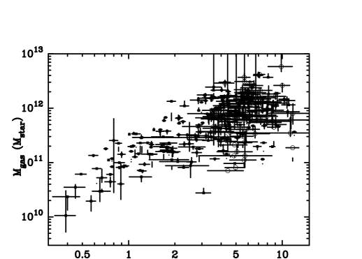
Figure 18: Gas mass against the gas temperature. The left panel plots the gas mass within 120$h_{50}^{-1}$ kpc. The symbols are the same as those in figure 12. The right panel plots the ratio of the gas mass of individual objects within $r_{1500}$ to the cluster-averaged one calculated from the relation of $1.0\times 10^{12}\left(kT/{\rm 1keV}\right)^{2.33}$, by denoting objects whose gas mass within 120$h_{50}^{-1}$ kpc is less than $5\times 10^{11}M_{\odot}$ as open circles.

5 Discussion

We analyzed about 300 objects of galaxy clusters, galaxy groups, and elliptical galaxies systematically with the ASCA data, especially the GIS data. Our results are free from systematic uncertainties, such as differences between instruments and analysis procedures. In addition, our sample includes a wide range of system temperatures from 0.4 keV to $\sim 12$ keV. Utilizing this sample, we performed correlation studies, and found several interesting phenomena. Here, we discuss them from the view point of evolution, hierarchical structure, and so on.

5.1 Two Breaks in the LT Relation

We found that the LT relation exhibits two breaks at around 1 keV and 3–4 keV. These two breaks are also indicated by the temperature dependence of other properties, such as the hot-gas mass, size, and gas fraction. Here, we discuss the origin and implication of the two breaks in the temperature dependences.

The break at around $kT\sim 1$ keV was already reported by Ponman et al. (1996), and so on, as well as the steep LT relation below $kT=1$ keV. Ponman et al. (1996) and Helsdon and Ponman (2000) suggested that this steep relation is due to galaxy feedback; lower-temperature systems were more strongly affected by non-gravity heating, and the gas has escaped or become thinner. Balogh, Babul, and Patton (1999) reproduced this steep relation in semi-analytical models. Alternatively, as described in the previous subsection, it is suggested that the X-ray emission of low-temperature objects is around the detection threshold, and is possibly lost at the outermost region for low-surface-brightness objects, and thus the X-ray luminosity may be underestimated (Mulchaey et al. 2000). Accordingly, the slope of the LT relation in lower temperature objects may possibly become as small as that of galaxy clusters. In fact, if we estimate the X-ray luminosity within the radius $r_{1500}$, rather than the detection radius, $R_{\rm limit}$, the luminosity of low-temperature objects significantly increases, while the luminosity of high-temperature objects slightly decreases. This behavior can be understood from figure 15. The slope of the LT relation becomes $2.56\pm 0.33$, $3.68\pm 0.37$, and $3.40\pm 0.59$, for ICM temperatures of $>4$ keV, 1.5–5 keV, and $<1.5$ keV, respectively. Thus, the break at $kT\sim$1 keV disappears. If this is true, the existence of undetected group-scale X-ray emission is necessary around X-ray faint elliptical galaxies; we discuss this possibility in the next subsection. We infer that the hot gas escaped from low-temperature objects and some fractions remain, but cannot be easily detected.

The second break at around $kT\sim$3–4 keV is inferred from the other ICM features. The entropy and temperature relation shown by Ponman, Cannon, and Navarro (1999) exhibits an excess entropy below 3–4 keV. The Si-to-Fe abundance ratio of the ICM is constant above 4 keV, while it decreases toward the lower temperature below 4 keV (Fukazawa et al. 1998). The iron-to-stellar mass ratio also follows the same trend (Fukazawa 1997; Finoguenov et al. 2000, 2001), reflecting the trend of the gas mass fraction that we present in this paper (figure 17). These three issues can be explained by the scenario that a significant amount of ICM was pushed out by the galactic wind at the early galaxy formation epoch, driven by the burst of a type-II supernovae. Accordingly, it is reasonable that the break point around $kT=$3–4 keV is seen in the LT relation. The slope of the LT relation above $kT>4$ keV is 2.34$\pm$0.29, close to 2.0 predicted by the theoretical scaling law, while that for objects with $1.5<kT<4$ keV is 3.74$\pm$0.10, significantly steep. Furthermore, a large scatter around $kT\sim$3–4 keV implies the coexistence of objects belonging to the higher-temperature classes in the flat LT relation and to the lower temperature in the steep LT relation. Considering these features, it is suggested that higher temperature objects are well-relaxed systems, and their non-gravity effect becomes negligible due to the large amount of gravitational energy. As a result, they follow a scaling law in the LT relation. On the other hand, lower-temperature objects have significantly sufferred non-gravity heating, such as galactic winds, and thus do not follow the scaling law. This scenario also explains the fact that there is a correlation of the gas mass between the center and outer regions (figure 16). The non-gravity effect prevented the gas from condensing in the potential, and, as a result, the gas density is lower over the cluster-scale.

In the bottom-up scenario, rich clusters with higher temperature are formed through mergers of poorer clusters. Such poorer objects are thought to belong to the lower-temperature classes with excess entropy. After merging, the excess entropy may be removed in the release of extra-gravitational energy by radiation and so on to achieve virial equilibrium. Cavaliere, Menci, and Tozzi (1997, 1999) presented the simulation and analytic calculation of the cluster evolution, where they considered the preheating, subsequent hierarchical merging, shock heating/compression, and a new hydrostatic equilibrium. They found that the slope of the LT relation is 5 for galaxy groups, 3 for rich clusters, and saturates toward 2 for the highest-temperature clusters. This trend is in good agreement with our results, and indicates that smaller systems suffer the merger effect, while larger systems do not, because of few merger events where comparable subclusters mix with eath other.

It has been said that the LT relation of clusters of galaxies is steeper than that predicted by the scaling theory, and thus several alternative scenarios are proposed, which take into account gravitational heating, radiative cooling, and so on (Muanwong et al. 2002; Tornatore et al. 2003). Most of these scenarios predict a steep LT relation over any cluster temperature. However, our results show that rich clusters with $kT>4$ keV at least satisfy the scaling relation. As shown in subsection 4.2, the hot-gas distribution of cluster-scale components is less concentrated for lower-temperature objects. Heating or cooling is a possible effect to explain this trend. Since not all of the rich clusters exhibit evidence of radiative cooling, we think that the heating effect is preferable. In order to reproduce our results, heating effects should not be so large as to have influence on the LT relation above $kT>4$ keV.

5.2 Gas Distribution and Two Component Models

Concerning the X-ray surface brightness, we found that many objects exhibit a double-$\beta$ model structure, especially for lower-temperature objects, while rich clusters and X-ray faint elliptical galaxies do not. Such a double-$\beta$ structure has already been found by Ikebe et el. (1996) and Mulchaey and Zabludoff (1998) for galaxy groups, and by Matsushita et al. (1998) for the X-ray bright elliptical galaxy NGC 4636. Even for rich clusters, Ikebe et al. (1997) and Xu et al. (1998) have suggested a double-$\beta$ structure, although the poor angular resolution of ASCA cannot distinguish between a double-$\beta$ model and a NFW-like cusp model. Following the suggestion of Ikebe et al. (1996) and Matsushita et al. (1998) together, it can be said that X-ray bright galaxy groups and X-ray bright elliptical galaxies consist of the same class of objects, which exhibit a double-$\beta$ model structure.

In figure 20, we plot the luminosity of the inner $\beta$-model component against the temperature, together with the total luminosity. It can be seen that the inner components and X-ray faint elliptical galaxies connect smoothly with each other, indicating that we might see the same type of X-ray hot gas. Accordingly, as described in subsection 4.4, two types of X-ray hot gas come out; two components of the double-$\beta$ model are associated with the potentials of the galaxy and cluster. The cluster component is dominant in rich clusters, and not seen in X-ray faint elliptical galaxies. The galaxy component is seen in elliptical galaxies and poor clusters, and not seen in rich clusters. The reason for this phenomenon might be due to the temperature dependence of the X-ray distribution of the cluster component. We have already showed that the central electron density of the outer component in the double-$\beta$ model is lower for lower-temperature objects. In other words, the X-ray surface brightness of the outer component becomes fainter for lower-temperature objects. Therefore, in lower-temperature objects, the cluster component cannot be detected and we can only observe the galaxy component, while in rich clusters, where hot gas of the cluster component is bright and the gravitational potential of the galaxy is relatively negligible, the hot gas of the galaxy component cannot be resolved. Sanderson et al. (2003) claimed that the properties of the X-ray halo of elliptical galaxies in their sample are different from those of galaxy clusters, and we also confirmed this trend for a larger sample. They attributed this difference to the earlier formation epoch than that of rich clusters. However, we suggest that the X-ray size of galaxy-scale hot gas is intrinsically compact due to the smaller scale of galaxy potential than that of the cluster-scale one.

Therefore, it is speculated that, even in X-ray faint elliptical galaxies, the group-scale hot gas exists, but it is too faint to detect. If this hypothesis is correct, we can claim the general view of elliptical galaxies; most elliptical galaxies associate the group-scale gravitational potential and thus hot gas, but the density of hot gas scatters widely. Figure 20 supports the above suggestion, indicating that, for objects with $kT<$1 keV, the hot-gas density at the maximum detection radius in the GIS data is higher than $10^{-4}$ cm^-3, and different by only several times from the central hot-gas density (figure 13). In other words, the X-ray surface brightness of extended group-scale hot gas for lower-temperature objects is around the detection threshold, and sometimes cannot be detected even if it exists. In this case, we cannot distinguish whether the extended group-scale hot gas exists or not by the present data, and Astro-E2 XIS with large effective area and low background level will provide an opportunity to do it.

Our sample lacks X-ray faint galaxy groups, and HCG 68 is the only object. The X-ray surface brightness of HCG 68 is centered on the elliptical galaxy NGC 5353, and can be fitted by a single-$\beta$ model. The maximam radius is at most 70$h_{50}^{-1}$ kpc, similar to that of X-ray faint elliptical galaxies. Therefore, at least the X-ray emission is not due to the group scale, but due to the galaxy scale for HCG 68. In ROSAT PSPC observations, the extent was reported to be $\sim 130h_{50}^{-1}$ kpc (Pildis et al. 1995), and thus group-scale X-ray hot gas is indicated. In any case, the X-ray emission of HCG 68 seems to be dominated by the galaxy component. Mulchaey (2000) indicated that, for the lower temperature galaxy groups, the X-ray emission becomes irregular and is dominated by individual member galaxies. The opposite cases are spiral-dominant galaxy groups, such as HCG 92 (Stephan’s Quintet) (Sulentic et al. 1995; Awaki et al. 1997), HCG 57 (Fukazawa et al. 2002), and HCG 16 (Besole et al. 2003). Since these systems do not contain a dominant elliptical galaxy, the X-ray hot gas of the galaxy-scale component is not bright. Alternatively, the X-ray emission is dominated by the faint diffuse component with a size of 100–200$h_{50}^{-1}$ kpc. This is naturally considered to be the group-scale hot gas. In summary, there are two types of X-ray faint objects. One is dominated by the elliptical galaxy in the X-ray emission, and the group-scale hot gas is hardly, or barely, confirmed. The other is a spiral-dominated system, where we can observe only the group-scale hot gas with very faint diffuse X-ray emission.

Figure 19: Bolometric luminosity against the gas temperature. The filled squares are the same as in figure 12, and the open circles represent the luminosity of the inner component in the double-$\beta$ model fitting.

Figure 20: Electron density at the maximum detection radius, $R_{\rm limit}$. The open circles represent the case where the emission is beyond the GIS field of view.

We suggest that X-ray faint galaxy groups and elliptical galaxies may contain an amount of hot gas that is as large as X-ray bright ones, and there would be a non-detected hot gas around them. How can we observe them? This depends on the temperature of the hot gas. In our scenario, such hot gas would be heated up by gravity as well as hot gas at the inner region; therefore, the temperature is thought to be 0.5–1 keV. In this case, the detection of thermal X-ray emission is the most possible case, but is quite difficult. In the ASCA data, the systematic uncertainty of the CXB intensity rather than the detector intrinsic background limits the sensitivity. Both a wide field of view and good imaging quality to resolve CXB into point sources are necessary, and such detectors are not presently being proposed for the future mission. The other situation is that the hidden hot-gas component is not virialized well, and the temperature is around $10^{4-6}K$. The detection of such a thermal emission is difficult, and absorption lines in the spectra of background objects are expected. This indication is claimed by Mulchaey et al. (1996b), and so on. However, we must explain why the hot gas in the outer region is not thermalized. As described in subsection 5.1, we showed that the small detection radius and low luminosity of X-ray faint systems are not due to the compactness of the hot-gas extent, but due to the detection sensitivity. Several numerical simulations show that the ICM is heated up by shock waves within a radius of $r_{500}$ (Evrard et al. 1996; Takizawa, Mineshige 1998). Therefore, it is reasonable to think that the hot-gas temperature is not so different from the inner region as objects whose detection radius is large.

5.3 Scatter of X-ray Luminosity of Galaxy Groups and Elliptical Galaxies

Ao far we suggested, two hot-gas components exist in lower temperature systems: a galaxy component and a group component. Considering these components, we discuss the scatter of the X-ray properties for elliptical galaxies and galaxy groups. As mentioned in subsection 5.1, we imply that these two systems are basically the same class of objects for hot gas and dark matter, and only the stellar distribution is different; stars in elliptical galaxies concentrate in one galaxy, while stars in galaxy groups separately locate in several galaxies. This difference may be due to whether the galaxies in the systems have merged or not. The scatter of the X-ray luminosity is mainly caused by the scatter of the hot-gas density for the group components and the brightness of the galaxy components. The origin of the former is related to the degree of heating, dark-matter concentration, system age, and so on, and may be explained in formation theories. On the other hand, the scatter of the X-ray brightness of the galaxy components is not simply understood. Matsushita (1997, 2001) showed that the hot-gas mass within the 4-times effective radius is systematically different between X-ray bright ones and X-ray faint ones. Therefore, the difference at such a small scale is thought to be attributed not to the group component, but to the cD elliptical galaxies. The compression of the galaxy hot-gas component by the high pressure of the group hot-gas component in X-ray bright ones, the escape of hot gas from X-ray faint ones, and so on, are considered, although we cannot investigate this issue with the ASCA data. High-resolution imaging with Chandra data will give an answer.

The authors thank an anonymous referee for a careful reading and many helpful comments. The authors acknowledge T. Takahashi and the ASCA image analysis working group (Takahashi et al. 1995). The authors are also grateful to the ASCA team for their help in the spacecraft operation and calibration. YF thanks Prof. T. Ohsugi for encouraging and supporting this study.

Figure 13: Gas-temperature dependence of the $\beta$-model parameters. The top, middle, and bottom panels show $\beta$, the core radius, and the central electron density, respectively. The left panels plot the results of single-$\beta$ model fittings. The right panels plot the results of double-$\beta$ model fittings for the objects listed in table 5 (open circle), together with those of single-$\beta$ model fittings for other objects (filled square).

Table 1: Sample list of clusters of galaxies.

Table 2: Results of spectral fittings.

Table 3: Results of radial profile fittings.

Table 4: Flux, central surface brightness, and luminosity.

Table 5: Results of radial profile fittings with double-$\beta$ model.

References

- [] Akritas, M. G., Bershady, M. A. 1996, ApJ, 470, 706
- [] Allen, S. W., & Fabian, A. C. 1998, MNRAS, 297, L57
- [] Anders, E., & Grevesse, N. 1989, Geochim. Cosmochim. Acta., 53, 197
- [] Arnaud, M., & Raymond, J. 1992, ApJ, 398, 394
- [] Awaki, H., Koyama, K., Matsumoto, H., Tomida, H., Tsuru,T., & Ueno, S. 1997, PASJ, 49, 445
- [] Balogh, M. L., Babul, A., & Patton, D. R. 1999, MNRAS, 307, 463
- [] Belsole, E., Sauvageot, J.-L., Ponman, T.J., & Bourdin, H. 2003, A&A, 398, 1
- [] Beuing, J., Döbereiner, S., Böhringer, H., & Bender, R. 1999, MNRAS, 302, 209
- [] Brown, B. A., & Bregman, J. N. 2000, ApJ, 539, 592
- [] Buote, D. A. 2000, MNRAS, 311, 176
- [] Cavaliere, A., & Fusco-Femiano, R. 1976, A&A, 49, 137
- [] Cavaliere, A., Menci, N., & Tozzi, P. 1997, ApJ, 484, L21
- [] Cavaliere, A., Menci, N., & Tozzi, P. 1999, MNRAS, 308, 599
- [] David, L. P., Jones, C., & Forman, W. 1995, ApJ, 445, 578
- [] David, L. P., Slyz, A., Jones, C., Forman, W., Vrtilek, S. D., & Arnaud, K. A. 1993, ApJ, 412, 479
- [] De Grandi, S., & Molendi, S. 2001, ApJ, 551, 153
- [] Dotani, T., et al. 1996, ASCA News, No.4, 3
- [] Edge, A. C., & Stewart, G. 1991, MNRAS, 252, 414
- [] Evrard, A. E. 1997, MNRAS, 292, 289
- [] Evrard, A. E., Metzler, C. A., & Navarro, J. F. 1996, ApJ, 469, 494
- [] Ezawa, H., Fukazawa, Y., Makishima, K., Ohashi, T., Takahara, F., Xu, H., & Yamasaki, N. Y. 1997, ApJ, 490, L33
- [] Fabian, A. C., Arnaud, K. A., Bautz, M. W., & Tawara, Y. 1994, ApJ, 436, L63
- [] Finoguenov, A., Arnaud, M., & David, L. P. 2001, ApJ, 555, 191
- [] Finoguenov, A., David, L. P., & Ponman, T. J. 2000, ApJ, 544, 188
- [] Fukazawa, Y. 1997, Ph D Thesis, The University of Tokyo
- [] Fukazawa, Y., et al. 1996, PASJ, 48, 395
- [] Fukazawa, Y., Kawano, N., Ohta, A., & Mizusawa, H. 2002, PASJ, 54, 527
- [] Fukazawa Y., Makishima, K., Tamura, T., Ezawa, H., Xu, H., Ikebe, Y., Kikuchi, K., & Ohashi, T. 1998 PASJ, 50, 187
- [] Fukazawa, Y., Makishima, K., Tamura, T., Nakazawa, K., Ezawa, H., Ikebe, Y., Kikuchi, K., & Ohashi, T. 2000 MNRAS, 313, 21
- [] Fukazawa, Y., Nakazawa, K., Isobe, N., Makishima, K., Matsushita, K., Ohashi, T., & Kamae, T. 2001, ApJ, 546, L87
- [] Helsdon, S. F., & Ponman, T. J. 2000, MNRAS, 319, 933
- [] Horner, D. J., Mushotzky, R. F., & Scharf, C. A. 1999, ApJ, 520, 78
- [] Ikebe, Y. 1995, Ph D Thesis, The University of Tokyo
- [] Ikebe, Y., et al. 1996, Nature, 379, 427
- [] Ikebe, Y., et al. 1997, ApJ, 481, 660
- [] Ishisaki, Y. 1996, Ph D Thesis, The University of Tokyo
- [] Ishisaki, Y., Ueda, Y., Kubo, H., Ikebe, Y., Makishima, K., and the GIS team 1997, ASCA News, No.5, 25
- [] Liedahl, D. A., Osterheld, A. L., & Goldstein, W. H. 1995, ApJ, 438, L115
- [] Loewenstein, M., & Mushotzky, R. F. 1996, ApJ, 471, L83
- [] Makishima, K., et al. 1996, PASJ, 48, 171
- [] Markevitch, M. 1998, ApJ, 504, 27
- [] Matsumoto, H., Koyama, K., Awaki, H., Tsuru, T., Loewenstein, M., & Matsushita, K. 1997 ApJ, 482, 133
- [] Matsumoto, H., Tsuru, T. G., Fukazawa, Y., Hattori, M., & Davis, D. S. 2000, PASJ, 52, 153
- [] Matsushita, K. 1997, Ph D Thesis, The University of Tokyo
- [] Matsushita, K. 2001, ApJ, 547, 693
- [] Matsushita, K., et al. 1994, PASJ, 52, 685
- [] Matsushita, K., Finoguenov, A., & Böhringer, H. 2003, A&A, 401, 443
- [] Matsushita, K., Makishima, K., Rokutanda, E., Yamasaki, N. Y., & Ohashi, T. 1997, ApJ, 488, L125
- [] Matsushita, K., Makishima, K., Ikebe, Y., Rokutanda, E., Yamasaki, N., & Ohashi, T. 1998, ApJ, 499, L13
- [] Mohr, J. J. & Evrard, A. E. 1997, ApJ, 491, 38
- [] Mohr, J. J., Mathiesen, B., & Evrard, A. E. 1999, ApJ, 517, 627
- [] Muanwong, O., Thomas, P. A., Kay, S. T., & Pearce, F. R. 2002, MNRAS, 336, 527
- [] Mulchaey, J. S. 2000, ARA&A, 38, 289
- [] Mulchaey, J. S., Davis, D. S., Mushotzky, R. F., & Burstein, D. 1996b, ApJ, 456, 80
- [] Mulchaey, J. S., Mushotzky, R. F., Burstein, D., & Davis, D. S. 1996a, ApJ, 456, L5
- [] Mulchaey, J. S., & Zabludoff, A. I. 1998, ApJ, 496, 73
- [] Mushotzky, R. F., Figueroa-Feliciano, E., Loewenstein, M., & Snowden S. L. 2003, astro-ph/0302267
- [] Mushotzky, R. F., & Loewenstein, M. 1997, ApJ, 481, L63
- [] Mushotzky, R. F., & Scharf, C. A. 1997, ApJ, 482, L13
- [] Navarro, J. F., Frenk, C. S., & White, S. D. M. 1995, MNRAS, 275, 720
- [] Ohashi, T., et al. 1996, PASJ, 48, 157
- [] O’Sullivan, E., Forbes, D. A., & Ponman, T. J. 2001, MNRAS, 328, 461
- [] Pildis, R. A., Bregman, J. N., & Evrard, A. E. 1995, ApJ, 443 514
- [] Ponman, T. J., Bourner, P. D. J., Ebeling, H., & Böhringer, H. 1996, MNRAS, 283, 690
- [] Ponman, T. J., Cannon, D. B., & Navarro, J. F. 1999, Nature, 397, 135
- [] Ponman, T. J., Sanderson, A. J. R., & Finoguenov, A. 2003, MNRAS, 343, 331
- [] Pratt, G. W., & Arnaud, M. 2003, A&A, 408, 1
- [] Raymond, J. C., & Smith, B. W. 1977, ApJS, 35, 419
- [] Renzini, A., Ciotti, L., D’Ercole, A., & Pellegrini, S. 1993, ApJ, 419, 52
- [] Sanderson, A. J. R., Ponman, T. J., Finoguenov, A., Lloyd-Davies, E. J., & Markevitch, M. 2003, MNRAS, 340, 989
- [] Stark, A. A., Gammie, C. F., Wilson, R. W., Bally, J., Linke, R. A., Heiles, C., & Hurwitz, M. 1992, ApJS, 79, 77
- [] Sulentic, J. W., Pietsch, W., & Arp, H. 1995, A&A, 298, 420
- [] Takahashi, T., Markevitch, M., Fukazawa, Y., Ikebe, Y., Ishisaki, Y., Kikuchi, K., Makishima, K., Tawara, Y., & ASCA Image analysis working group 1995, ASCA News, No.3, 34
- [] Takizawa, M., & Mineshige, S. 1998, ApJ, 499, 82
- [] Tanaka, Y., Inoue, H., & Holt, S. S. 1994, PASJ, 46, L37
- [] Tornatore, L., Borgani, S., Springel, V., Matteucci, F., Menci, N., & Murante, G. 2003, MNRAS, 342, 1025
- [] Tozzi, P., & Norman, C. 2001, ApJ, 546, 63
- [] Ueda, Y. 1996, Ph D Thesis, The University of Tokyo
- [] Ueda, Y., et al. 1999, ApJ, 518, 656
- [] Wu, X.-P., Xue, Y.-J., & Fang, L.-Z. 1999, ApJ, 524, 22
- [] Xu, H., Makishima, K., Fukazawa, Y., Ikebe, Y., Kikuchi, K., Ohashi, T., & Tamura, T. 1998, ApJ, 500, 738
- [] Xue, Y.-J., & Wu, X.-P. 2000, ApJ, 538, 65