Introduction to galactic dynamos

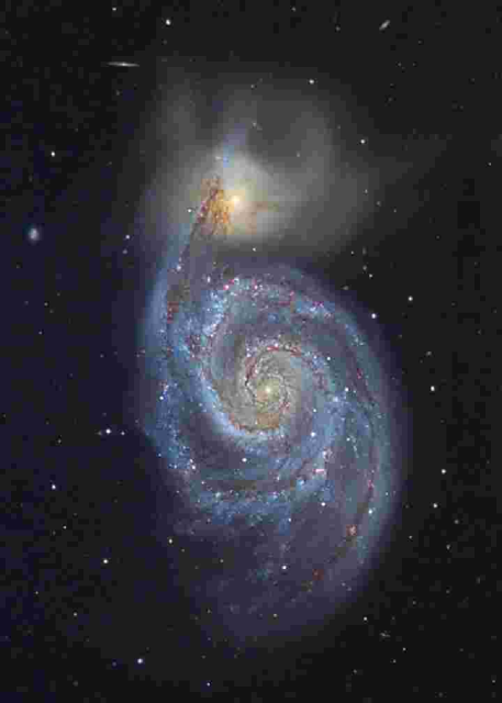
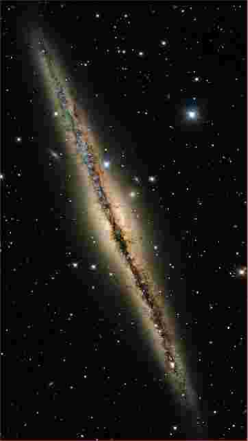
Figure 1: Optical images of two nearby spiral galaxies. Left: M51, the Whirlpool galaxy (with a satellite galaxy at the top). Right: NGC 891 (Courtesy of the Canada–France–Hawaii Telescope/J.-C. Cuillandre/Coelum). M51 is one of nearby galaxies (distance 9.6 Mpc) notable for its prominent spiral pattern. M51 is the first galaxy where a well ordered, large-scale magnetic field was detected (Segalovitz et al., 1976) and studied in fine detail. NGC 891 is at about the same distance as M51, but seen nearly edge-on, so the thinness of the galactic disc is evident. The dark strip along the galactic disc and filaments extended away from the galactic plane are due to obscuration by interstellar dust. The filaments trace gas outflow from the disc into the halo.

1 Introduction

Galaxies are attractive objects to study. The magnetism of their natural beauty adds to the fascinating diversity of physical processes that occur over an enormous range of scales from the global dimension of order 10 kpc down to the viscous turbulent scales of 1000 km and less. The visual image of a galaxy (see Fig. 1) is dominated by the optical light mostly produced by stars that contribute most of the visible galactic mass ($2\times 10^{11}M_{\odot}$ for the Milky Way, where $M_{\odot}=2\times 10^{30}\,{\rm kg}$ is the mass of the Sun). A few percent of the galactic mass is due to the interstellar gas that resides in the gravitational field produced by stars and dark matter. Spiral galaxies are flat (Fig. 1) because the stars and gas rapidly rotate. The gas is ionized by the UV and X-ray radiation and by cosmic rays; the degree of ionization of diffuse gas ranges from 30% to 100% in various phases — see Sect. 2.1). Interstellar gas is involved in turbulent motions that can be detected because the associated Doppler shifts broaden spectral lines emitted by the gas beyond their width expected from thermal motions alone. The effective mean free path of interstellar gas particles is small enough to justify a fluid description under a broad range of conditions. Altogether, interstellar gas can be reasonably described as an electrically conducting, rotating, stratified turbulent fluid — and thus a site of MHD processes discussed elsewhere in this volume, including various types of dynamo action.

The energy density of interstellar magnetic fields is observed to be comparable to the kinetic energy density of interstellar turbulence and cosmic ray energy density, and apparently exceeds the thermal energy density of interstellar gas (Cox, 1990). Therefore, interstellar gas, magnetic field and cosmic rays form a complex, nonlinear physical systems whose behaviour is equally affected by each of the three components. The system is so complex that magnetic fields and cosmic rays — the components that are more difficult to observe and model — are often neglected. Such a simplification is perhaps justifiable at very large scales of order 10 kpc, where the motions of interstellar gas (mainly the overall rotation) are governed by gravity: systematic motions at a speed in excess of 10–$30\,{\rm km\,s^{-1}}$ are too strong to be affected by interstellar magnetic fields. However, motions at smaller scales (comparable to and less than the turbulent scale, $\ell\approx 0.1\,{\rm kpc}$) are strongly influenced by magnetic fields. In particular, interstellar turbulence is in fact an MHD turbulence. In this respect, the interstellar environment does not differ much from stellar and planetary interiors.

Until recently, interstellar magnetic fields had been a rather isolated area of galactic astrophysics. The reason for that was twofold. Firstly, magnetic fields are difficult to observe and model. Secondly, they were understood too poorly to provide useful insight into the physics of interstellar gas and galaxies in general. The widespread attitude of galactic astrophysicists to interstellar magnetic fields was succinctly described by Woltjer (1967):

The argument in the past has frequently been a process of elimination: one observed certain phenomena, and one investigated what part of the phenomena could be explained; then the unexplained part was taken to show the effects of the magnetic field. It is clear in this case that, the larger one’s ignorance, the stronger the magnetic field.

The attitude hardly changed in 20 subsequent years, when Cox (1990) observed that

As usual in astrophysics, the way out of a difficulty is to invoke the poorly understood magnetic field. …One tends to ignore the field so long as one can get away with it.

The situation has changed dramatically over the last 10–15 years. Theory and observations of galactic magnetic fields are now advanced enough to provide useful constraints on the kinematics and dynamics of interstellar gas, and the importance and rôle of galactic magnetic fields are better appreciated.

In this chapter, we review in Sect. 2 those aspects of galactic astrophysics that are relevant to magnetic fields, and briefly summarize in Sect. 3 our observational knowledge of magnetic fields in spiral galaxies. Section 4 is an exposition of the current ideas on the origin of galactic magnetic fields, including the dynamo theory. The confrontation of theory with observations is the subject of Sect. 5 where we summarize the advantages and difficulties of various theories and argue that the mean-field dynamo theory remains the best contender. Magnetic fields in elliptical galaxies are briefly discussed in Sect. 6.

2 Interstellar medium in spiral galaxies

2.1 Turbulence and multi-phase structure

The interstellar medium (ISM) is much more inhomogeneous and active than stellar and planetary interiors. The reason for that is ongoing star formation where massive young stars evolve rapidly (in about $10^{6}\,{\rm yr}$) and then explode as supernova stars (SN) releasing large amounts of energy ($E_{\mathrm{SN}}\sim 10^{51}\,{\rm erg}$ per event). These explosions control the structure of the ISM.

SN remnants are filled with hot, overpressured gas and first expand supersonically; at this stage the gas surrounding the blast wave is not perturbed. However, a pressure disturbance starts propagating faster than the SN shell as soon as the expansion velocity becomes comparable to or lower than the speed of sound in the surrounding gas — at this stage the expanding SN remnant drives motions in the surrounding gas, and its energy is partially converted into the kinetic energy of the ISM. When pressure inside an SN remnant reduces to values comparable to that in the surrounding gas, the remnant disintegrates and merges with the ISM. Since SN occur at (almost) random times and positions, the result is a random force that drives random motions in the ISM that eventually become turbulent. The size of an SN remnant when it has reached pressure balance determines the energy-range turbulent scale,

$$\ell\approx 0.05\mbox{--}0.1\,{\rm kpc}.$$

A useful review of supernova dynamics can be found, e.g., in Lozinskaya (1992), and the spectral properties of interstellar turbulence are discussed by Armstrong et al. (1995). Among numerous reviews of the multi-phase ISM we mention that of Cox (1990) and a recent text of Dopita & Sutherland (2003).

About $f=0.07$ of the SN energy is converted into the ISM’s kinetic energy. With the SN frequency of $\nu_{\mathrm{SN}}\sim(30\,{\rm yr})^{-1}$ in the Milky Way (i.e., one SN per $30\,{\rm yr}$), the kinetic energy supply rate per unit mass is $\dot{e}_{\mathrm{SN}}=f\nu_{\mathrm{SM}}E_{\mathrm{SN}}M_{\mathrm{gas}}^{-1}\sim 10^{-2}\,{\rm erg}\,{\rm g}^{-1}\,{\rm s}^{-1}$, where $M_{\mathrm{gas}}=4\times 10^{9}\,M_{\odot}$ is the total mass of gas in the galaxy. This energy supply can drive turbulent motions at a speed $u_{0}$ such that $2u_{0}^{3}/\ell=\dot{e}_{\mathrm{SN}}$ (where the factor 2 allows for equal contributions of kinetic and magnetic turbulent energies), which yields

$$u_{0}\sim 10\mbox{--}30\,{\rm km\,s^{-1}},$$

a value similar to the speed of sound at a temperature $T=10^{4}\,{\rm K}$ or higher. The corresponding turbulent diffusivity follows as

$$\eta_{\rm T}\sim{\textstyle{\frac{1}{3}}}\ell u_{0}\approx(0.5\mbox{--}3)\times 10^{26}\,{\rm cm}^{2}\,{\rm s}^{-1}\;.$$ (1)

Supernovae are the main source of turbulence in the ISM. Stellar winds is another significant source, contributing about 25% of the total energy supply (e.g., §VI.3 in Ruzmaikin et al., 1988).

The time interval between supernova shocks passing through a given point is about (McKee & Ostriker, 1977; Cox, 1990)

$$\tau=(0.5\mbox{--}5)\times 10^{6}\,{\rm yr}.$$

After this period of time, the velocity field at a given position completely renovates to become independent of its previous form. Therefore, this time can be identified with the correlation time of interstellar turbulence. The renovation time is 2–20 times shorter than the ‘eddy turnover’ time $\ell/u_{0}\sim 10^{7}\,{\rm yr}$. This means that the short-correlated (or $\delta$-correlated) approximation, so important in turbulence and dynamo theory (e.g., Zeldovich et al., 1990; Brandenburg & Subramanian, 2004), can be quite accurate in application to the ISM — this is a unique feature of interstellar turbulence. Note that the standard estimate (1) is valid if the correlation time is $\ell/u_{0}$. If the renovation time was used instead, the result would be $\eta_{\rm T}\sim\ell^{2}/\tau\sim 10^{27}\,{\rm cm}^{2}\,{\rm s}^{-1}$, a value an order of magnitude larger than the standard estimate.

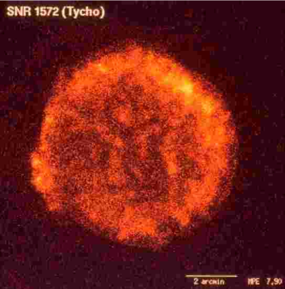
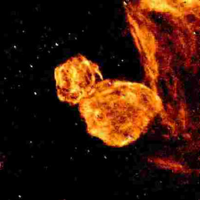
Figure 2: SN remnants are expanding bubbles of hot gas that emits thermal X-rays. This is illustrated by the X-ray image of Tycho’s supernova remnant (left panel; courtesy of the ROSAT Mission and the Max-Planck-Institut für extraterrestrische Physik) whose parent star’s explosion in 1572 was recorded by the famous Danish astronomer Tycho Brahe. The hot gas cools only slowly, and SN remnants often merge. The right panel shows a false-colour optical (H$\alpha$) image of two SN remnants DEM L316 in the Large Magellanic Cloud which appear to be colliding (Williams et al., 1997; image produced by the Magellanic Cloud Emission-Line Survey, reprinted with permission).

Table 1: The multi-phase ISM. The origin and parameters of the most important phases of interstellar gas: $n$, the mid-plane number density in hydrogen atoms per cm³; $T$, the temperature in K; $c_{\mathrm{s}}$, the speed of sound in km s^-1; $h$, the scale height in kpc; and $f_{V}$, the volume filling factor in the disc of the Milky Way, in per cent.

Phase	Origin	$n$	$T$	$c_{\mathrm{s}}$	$h$	$f_{V}$
Warm		0.1	$10^{4}$	10	0.5	60–80
Hot	Supernovae	$10^{-3}$	$10^{6}$	100	3	20–40
Hydrogen clouds	Compression	20	$10^{2}$	1	0.1	2
Molecular clouds	Self-gravity,	$10^{3}$	10	0.3	0.075	0.1
	thermal instability

Another important result of supernova activity is a large amount of gas heated to $t=10^{6}\,{\rm K}$ (Fig. 2). The gas is so tenuous that the collision rate of the gas particles is low, and so its radiative cooling time is very long and exceeds $\tau$: the hot bubbles produced by supernovae can merge before they cool (Fig. 2). A result is a network of hot tunnels that form the hot component of the ISM. Altogether, the interstellar gas is found in several distinct states, known as ‘phases’ (this usage may be misleading as most of them are not proper thermodynamic phases) whose parameters are presented in Table 1. Some of the parameters (especially the volume filling factors) are not known confidently, so estimates of Table 1 should be approached with healthy skepticism. The warm diffuse gas can be considered as a background against which the ISM dynamics evolves; this is the primary phase that occupies a connected (percolating) region in the disc, whereas the hot gas may or may not fill a connected region. The warm gas is ionized by the stellar ultraviolet radiation and cosmic rays; its degree of ionization is about 30% at the Galactic midplane. The hot gas is so hot that it is fully ionized by gas particle collisions.

The locations of SN stars are not entirely random: 70% of them cluster in regions of intense star formation (known as OB associations as they contain large numbers of young, bright stars of spectral classes O and B) where gas density is larger than on average in the galaxy. Collective energy input from a few tens (typically, 50) SN within a region about 0.5–1 kpc in size produces a superbubble that can break through the galactic disc (Tenorio-Tagle & Bodenheimer, 1988). This removes the hot gas into the galactic halo and significantly reduces its filling factor in the disc (from about 70% to 10–20%). This also gives rise to a systematic outflow of the hot gas to large heights where the gas eventually cools, condenses and returns to the disc after about $10^{9}\,{\rm yr}$ in the form of cold, dense clouds of neutral hydrogen (Wakker & van Woerden, 1997). This convection-type flow is known as the galactic fountain (Shapiro & Field, 1976), and it can plausibly support a mean-field dynamo of its own (Sokoloff & Shukurov, 1990). Another aspect of its rôle in galactic dynamos is discussed in Sect. 4.3. The vertical velocity of the hot gas at the base of the fountain flow is 100–$200\,{\rm km\,s^{-1}}$ (e.g., Kahn & Brett, 1993; Korpi et al., 1999a,b).

2.2 Galactic rotation

Spiral galaxies have conspicuous flat components because they rotate rapidly enough. The Sun moves in the Milky Way at a velocity of about $u_{\odot}=s_{\odot}\Omega_{\odot}=220\,{\rm km\,s^{-1}}$, to complete one orbit of a radius $s_{\odot}\approx 8.5\,{\rm kpc}$ in $2\pi/\Omega_{\odot}=2.4\times 10^{8}\,{\rm yr}$. These values are representative for spiral galaxies in general. The Rossby number is estimated as

$$\mbox{Ro}=\frac{u_{0}}{\ell\Omega_{\odot}}\sim 4\;.$$

The vertical distribution of the gas is controlled, to the first approximation, by hydrostatic equilibrium in the gravity field produced by stars and dark matter, with pressure comprising thermal, turbulent, magnetic and cosmic ray components in roughly equal proportion (e.g., Boulares & Cox, 1990; Fletcher & Shukurov, 2001). The semi-thickness of the warm gas layer is about $h=0.5\,{\rm kpc}$, i.e., the aspect ratio of the gas disc is

$$\mbox{$\varepsilon$}=\frac{h}{s_{\odot}}\sim 0.06\;.$$ (2)

Since the gravity force decreases with radius $s$ together with the stellar mass density, $h$ grows with $s$ at $s\;\raise 1.29167pt\hbox{$>$\kern-7.5pt\raise-4.73611pt\hbox{$\sim$}}\;\hskip-2.0pt10\,{\rm kpc}$ (see §VI.2 in Ruzmaikin et al., 1988, for a review).

However, the hot gas has larger speed of sound and turbulent velocity, and its Rossby number can be as large as 10 given that its turbulent scale is about $0.3\,{\rm kpc}$ (see Poezd et al., 1993). Hence, the hot gas fills a quasi-spherical volume, where its pressure scale height of order $5\,{\rm kpc}$ is comparable to the disc radius.

$\mbox{Ro}=1$ at a scale $0.4\,{\rm kpc}$ in the warm gas, which is similar to the scale height of the gas layer. This implies that rotation significantly affects turbulent gas motions, making them helical on average. A convenient estimate of the associated $\alpha$-effect can be obtained from Krause’s formula,

$$\alpha_{0}\sim\frac{\ell^{2}\Omega}{h}\approx 0.5\,{\rm km\,s^{-1}}\;,$$ (3)

where $\Omega$ is the angular velocity, and the numerical estimate refers to the Solar neighbourhood of the Milky Way. Thus, $\alpha_{0}\sim 0.05u_{0}$ near the Sun and increases in the inner Galaxy together with $\Omega$.

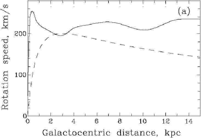
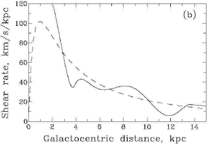
Figure 3: (a): The rotation speed $s\Omega(s)$ in the galactic midplane versus galactocentric radius $s$ in the Milky Way (solid) (Clemens, 1985), and the generic Schmidt’s rotation curve with $U_{0}=200\,{\rm km\,s^{-1}}$, $s_{0}=3\,{\rm kpc}$ and $n=1$ (dashed). (b): The corresponding rotation shear rates (taken with minus sign), $-s\partial\Omega/\partial s$.

The spatial distribution of galactic rotation is known for thousands galaxies (Sofue & Rubin, 2001) from systematic Doppler shifts of various spectral lines emitted by stars and gas. In this respect, galaxies are much better explored than any star or planet (including the Sun and the Earth) where reliable data on the angular velocity in the interior are much less detailed and reliable or even unavailable. The radial profile of the galactic rotational velocity is called the rotation curve. Rotation curves of most galaxies are flat beyond a certain distance from the axis, so $\Omega\propto s^{-1}$ is a good approximation for $s\;\raise 1.29167pt\hbox{$>$\kern-7.5pt\raise-4.73611pt\hbox{$\sim$}}\;\hskip-2.0pt5\,{\rm kpc}$. The rotation curve of a generic galaxy, known as the Schmidt rotation curve and shown in Fig. 3, has the form

$$s\Omega(s)=U_{0}\frac{s}{s_{0}}\left[{\textstyle{\frac{1}{3}}}+{\textstyle{\frac{2}{3}}}\left(\frac{s}{s_{0}}\right)^{n}\right]^{-3/2n}\;,$$

where the parameters vary between various galaxies in the range $s_{0}\sim 5$–$20\,{\rm kpc}$, $U_{0}\sim 200\,{\rm km\,s^{-1}}$ and $n\sim 0.7$–1. This rotation curve is not flat at large radii, but it provides an acceptable approximation at moderate distances from galactic centre where magnetic field generation is most intense. Some galaxies have more complicated rotation curves. Notably, the Milky Way and M31 are among them — see Figs 3 and 5. The complexity of the rotation curves is explained by a complicated distribution of the gravitating (stellar and dark) mass in those galaxies. It is evident from Fig. 3b that the rotation shear is strong at all radii even for the Schmidt rotation curve, and so the rotation in the inner part of a spiral galaxy cannot be approximated by the solid-body law, even if the shape of some rotating curves tempts to do so.

The vertical variation of the rotation velocity is only poorly known. In a uniform gravitating disc of infinite radial extent the angular velocity of rotation would be constant in $z$. Then it is natural to expect that $\Omega$ should decrease along $z$ at a scale comparable to the radial scale length of the gravitating mass in the disc, typically $s_{*}=3$–$5\,{\rm kpc}$. Recent observations of gas motions in galactic halos have confirmed such a decrease (Fraternali et al., 2003). In the absence of detailed models, an approximation $\Omega\propto\mathrm{exp}\,(-z/s_{*})$ seems to be appropriate.

3 Magnetic fields observed in galaxies

Estimates of magnetic field strength in the diffuse interstellar medium of the Milky Way and other galaxies are most efficiently obtained from the intensity and Faraday rotation of synchrotron emission. Other methods are only sensitive to relatively strong magnetic fields that occur in dense clouds (Zeeman splitting) or are difficult to quantify (optical polarization of star light by dust grains). The total $I$ and polarized $P$ synchrotron intensities and the Faraday rotation measure ${\rm RM}$ are weighted integrals of magnetic field over the path length $L$ from the source to the observer, so they provide a measure of the average magnetic field in the emitting or magneto-active volume:

$$I = K\int_{L}n_{\rm cr}B_{\perp}^{2}\,ds\;,$$

$$P = K\int_{L}n_{\rm cr}\overline{B}_{\perp}^{2}\,ds\;,$$ (4)

$${\rm RM} = K_{1}\int_{L}n_{\rm e}B_{\parallel}\,ds\;,$$

where $n_{\rm cr}$ and $n_{\rm e}$ are the number densities of relativistic and thermal electrons, ${\bf B}$ is the total magnetic field comprising a regular $\overline{{\bf B}}$ and random ${\bf b}$ parts, ${\bf B}=\overline{{\bf B}}+{\bf b}$ with $\langle{\bf B}\rangle=\overline{{\bf B}},\ \langle{\bf b}\rangle=0$ and $\langle{B^{2}}\rangle=B^{2}+\langle b^{2}\rangle$, angular brackets denote averaging, subscripts $\perp$ and $\parallel$ refer to magnetic field components perpendicular and parallel to the line of sight, and $K$ and $K_{1}=e^{3}/(2\pi\,{\rm m}_{\mathrm{e}}^{2}c^{4})=0.81\,{\rm rad\,m^{-2}}\,{\rm cm}^{3}\,\mu{\rm G}^{-1}\,{\rm pc}^{-1}$ are certain dimensional constants (with $e$ amd $m_{\mathrm{e}}$ the electron charge and mass and $c$ the speed of light). The degree of polarization $p$ is related to the ratio $\langle b^{2}\rangle/\overline{B}^{2}$,

$$p\equiv\frac{P}{I}\approx p_{0}\frac{\overline{B}_{\perp}^{2}}{B_{\perp}^{2}}=p_{0}\frac{\overline{B}_{\perp}^{2}}{\overline{B}_{\perp}^{2}+{\textstyle{\frac{2}{3}}}\langle b^{2}\rangle}\;,$$ (5)

where the random field ${\bf b}$ has been assumed to be isotropic in the last equality, $n_{\rm cr}$ is assumed to be a constant, and $p_{0}\approx 0.75$ weakly depends on the spectral index of the emission. This widely used relation is only approximate. In particular, it does not allow for any anisotropy of the random magnetic field, for the dependence of $n_{\mathrm{cr}}$ on $B$, and for depolarization effects; some generalizations are discussed by Sokoloff et al. (1998).

The orientation of the apparent large-scale magnetic field in the sky plane is given by the observed $B$-vector of the polarized synchrotron emission. Due to Faraday rotation, the true orientation can differ by an angle of ${\rm RM}\lambda^{2}$, which amounts to $10^{\circ}$–$20^{\circ}$ at a wavelength $\lambda=6\,{\rm cm}$. The special importance of the Faraday rotation measure, ${\rm RM}$, is that this observable is sensitive to the direction of ${\bf B}$ (the sign of $\overline{B}_{\parallel}$) and this allows one to determine not only the orientation of $\overline{{\bf B}}$ but also its direction. Thus, analysis of Faraday rotation measures can reveal the three-dimensional structure of the magnetic vector field (Berkhuijsen et al., 1997; Beck et al., 1996).

Since $n_{\rm cr}$ is difficult to measure, it is often assumed that magnetic field and cosmic rays are in pressure equilibrium or energy equipartition; this allows to express $n_{\rm cr}$ in terms of $B$. The physical basis of this assumption is the fact that cosmic rays (charged particles of relativistic energies) are confined by magnetic fields. An additional assumption involved is that the energy density of relativistic electrons responsible for synchrotron emission (energy of several GeV per particle) is one percent of the proton energy density in the same energy interval, as measured near the Earth.

The cosmic ray number density$n_{\rm cr}$ in the Milky Way can be determined independently from $\gamma$-ray emission produced when cosmic ray particles interact with the interstellar gas. Then magnetic field strength can be obtained without assuming equipartition (Strong et al., 2000); the results are generally consistent with the equipartition values. However, Eq. (5) is not consistent with the equipartition or pressure balance between cosmic rays and magnetic fields as it assumes that $n_{\rm cr}=\mbox{const}$. Therefore, $\overline{B}$ obtained from Eq. (5) can be inaccurate (Beck et al., 2003).

The mean thermal electron density $n_{\rm e}$ in the ISM can be obtained from the emission measure of the interstellar gas, an observable defined as ${\rm EM}\propto\int_{L}n_{\rm e}^{2}\,ds$, but this involves the poorly known filling factor of interstellar clouds. In the Milky Way, the dispersion measures of pulsars, ${\rm DM}=\int_{L}n_{\rm e}\,ds$ provide information about the mean thermal electron density, but the accuracy is limited by our uncertain knowledge of distances to pulsars. Estimates of the strength of the regular magnetic field in the Milky Way are often obtained from the Faraday rotation measures of pulsars simply as

$$B_{\parallel}=\frac{{\rm RM}}{K_{1}\,\rm DM}\;.$$ (6)

This estimate is meaningful if magnetic field and thermal electron density are statistically uncorrelated. If the fluctuations in magnetic field and thermal electron density are correlated with each other, they will contribute positively to ${\rm RM}$ and Eq. (6) will yield overestimated $\overline{B}_{\parallel}$. In the case of anticorrelated fluctuations, their contribution is negative and Eq. (6) is an underestimate. As shown by Beck et al. (2003), physically reasonable assumptions about the statistical relation between magnetic field strength and electron density can lead to Eq. (6) being in error by a factor of 2–3.

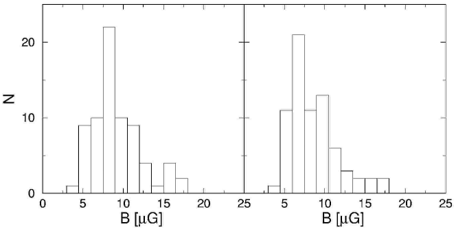
Figure 4: The distributions of the strength of the total magnetic field in a sample of spiral galaxies obtained from the observed synchrotron intensity $I$ using energy equipartition between magnetic fields and cosmic rays (p. 109 in Niklas, 1995) under slightly different assumptions. The estimates of the left-hand panel were derived from integrating the observed synchrotron intensity in the range corresponding to the relativistic electron energies from 300 MeV to infinity, and in the right-hand panel the integration was over a frequency range 10 MHz–10 GHz. Results presented in the left-hand panel are better justified physically (§2.1 in Beck et al., 1996; §III.A.1 in Widrow, 2002).

The observable quantities (4) have provided extensive data on magnetic field strengths in both the Milky Way and external galaxies (Ruzmaikin et al.., 1988; Beck et al., 1996; Beck, 2000, 2001). The average total field strengths in nearby spiral galaxies obtained from total synchrotron intensity $I$ range from $B\approx 4\,\mu{\rm G}$ in the galaxy M31 to about $15\,\mu{\rm G}$ in M51, with the mean for the sample of 74 galaxies of $B=9\,\mu{\rm G}$ (Beck, 2000). Figure 4 shows the distribution of magnetic field strength in a sample of spiral galaxies. The typical degree of polarization of synchrotron emission from galaxies at short radio wavelengths is $p=10$–$20\%$, so Eq. (5) gives $\overline{B}/B=0.4$–0.5; these are always lower limits due to the limited resolution of the observations, and $\overline{B}/B=0.6$–0.7 is a more plausible estimate. Most existing polarization surveys of synchrotron emission from the Milky Way, having much better spatial resolution, suffer from Faraday depolarization effects and missing large-scale emission and cannot provide reliable values for $p$. The total equipartition magnetic field in the Solar neighbourhood is estimated as $B=6\pm 2\,\mu{\rm G}$ from the synchrotron intensity of the diffuse Galactic radio background (E. M. Berkhuijsen, in Beck, 2001). Combined with $\overline{B}/B=0.65$, this yields a strength of the local regular field of $\overline{B}=4\pm 1\,\mu{\rm G}$. Hence, the typical strength of the local Galactic random magnetic fields, $b=(B^{2}-\overline{B}^{2})^{1/2}=5\pm 2\,\mu{\rm G}$, exceeds that of the regular field by a factor $b/\overline{B}=1.3\pm 0.6$. ${\rm RM}$ data yield similar values for this ratio (§IV.4 in Ruzmaikin et al., 1988).

Meanwhile, the values of $\overline{B}$ in the Milky Way obtained from Faraday rotation measures seem to be systematically lower than the above values (see Beck et al., 2003, and references therein). ${\rm RM}$ of pulsars and extragalactic radio sources yield $\overline{B}=1$–$2\,\mu{\rm G}$ in the Solar vicinity, a value about twice smaller than that inferred from the synchrotron intensity and polarization. There can be several reasons for the discrepancy between the estimates of the regular magnetic field strength from Faraday rotation and synchrotron intensity. Both methods suffer from systematic errors due to our uncertain knowledge of thermal and relativistic electron densities, so one cannot be sure if the difference is significant. Nevertheless, the discrepancy seems to be worrying enough to consider carefully its possible reasons.

The discrepancy can be explained, at least in part, if the methods described above sample different volumes. The observation depth of total synchrotron emission, starlight polarization and of Faraday rotation measures are all of the order of a few kpc. Polarized emission, however, may emerge from more nearby regions. However, a more fundamental reason for the discrepancy can be partial correlation between fluctuations in magnetic field and electron density. Such a correlation can arise from statistical pressure balance where regions with larger gas density have weaker magnetic field, and vice versa. As discussed by Beck et al. (2003), the term $\langle b_{\parallel}n_{\rm e}\rangle$ then differs from zero and contributes to the observed ${\rm RM}$ leading to underestimated $\overline{B}$. In a similar manner, correlation between $B$ and the cosmic ray number density biases the estimates of magnetic field from synchrotron intensity and polarization (see also Sokoloff et al., 1998). Altogether, $\overline{B}=4\,\mu{\rm G}$ and $b=5\,\mu{\rm G}$ seem to be acceptable estimates of magnetic field strengths near the Sun. The geometry and three-dimensional structure of the magnetic fields observed in spiral galaxies are further discussed in Sect. 5.

4 The origin of galactic magnetic fields

There are two basic approaches to the origin of global magnetic structures in spiral galaxies — one of them asserts that the observed structures represent a primordial magnetic field twisted by differential rotation, and the other that they are due to ongoing dynamo action within the galaxy. The simplicity of the former theory is appealing, but it fails to explain the strength, geometry and apparent lifetime of galactic magnetic fields (Ruzmaikin et al., 1988; Beck et al., 1996; Kulsrud, 1999; Widrow, 2002; see Sect. 5 below). Furthermore, there are no mechanisms known to produce cosmological magnetic fields of required strength and scale (Beck et al., 1996), although Kulsrud et al. (1997) argue that suitable magnetic field can be produced in protogalaxies. Dynamo models appear to be much better consistent with the observational and theoretical knowledge of interstellar gas, and all models of magnetic fields in specific galaxies, known to the author, have been formulated in terms of dynamo theory. It seems to be very plausible that galactic magnetic fields are generated by some kind of dynamo action, i.e., that they are produced in situ. The most promising is the mean-field turbulent dynamo.

4.1 Mean-field models of the galactic dynamo

As discussed in Sect. 2.2, the discs of spiral galaxies are thin. This provides a natural small parameter, the disc aspect ratio, Eq. (2). This greatly facilitates modelling of many global phenomena in galaxies, including large-scale magnetic fields. Parker (1971) and Vainshtein & Ruzmaikin (1971, 1972) were the first to suggest mean-field dynamo models for spiral galaxies. These were local models discussed in Sect. 4.1.2, where only derivatives across the disc (in $z$) are retained. The theory has been extended to two and more dimensions and applied to specific galaxies (see Ruzmaikin et al., 1988, Beck et al., 1996, and Widrow, 2002, and references therein). Rigorous asymptotic solutions for the $\alpha\omega$-dynamo in a thin disc were developed by Soward (1978, 1992a,b) and further discussed by Priklonsky et al. (2000) and Willis et al. (2003). Reviews of these results can be found in Ruzmaikin et al. (1988), Beck et al. (1996), Kulsrud (1999) and Soward (2003).

In this section we present asymptotic solutions of the mean-field dynamo equations in a thin disc surrounded by vacuum. We first consider axially symmetric solutions of the kinematic problem, and then discuss generalizations to non-axisymmetric modes and to nonlinear regimes. Cylindrical coordinates $(s,\phi,z)$ with the origin the galactic centre and the $z$-axis parallel to the galactic angular velocity are used throughout this chapter. In this section we use dimensionless variables, with $s$ and $z$ measured in the units of the characteristic disc radius and disc half-thickness (e.g., $s_{0}=s_{\odot}\approx 8.5\,{\rm kpc}$ and $h_{0}=0.5\,{\rm kpc}$), respectively. Then the dimensionless radial and axial distances are both of order unity within the disc as they are measured in different units in order to make the disc thinness explicit. The corresponding time unit is the turbulent magnetic diffusion time across the disc, $h_{0}^{2}/\eta_{\rm T}\approx 7.5\times 10^{8}\,{\rm yr}$.

It is convenient to introduce a unit rotational shear rate $G_{0}$,

$$G=s\frac{\partial\Omega}{\partial s}\equiv G_{0}g(s,z)\;,$$

with $g(s,z)$ its dimensionless value and $G_{0}=-\Omega_{\odot}$ for a flat rotation curve, $\Omega\propto s^{-1}$, and adopt the characteristic magnitude of the $\alpha$-coefficient near the Sun as given by Eq. (3).

4.1.1 Kinematic, axially symmetric solutions

The three components of an axially symmetric magnetic field can be expressed in terms of the azimuthal components of the large-scale magnetic field $\overline{B}_{\phi}$ and vector potential $\overline{A}_{\phi}$,

$$\overline{{\mbox{\bf B}}}=\left(-\frac{\partial\overline{A}_{\phi}}{\partial z},\ \overline{B}_{\phi},\ \frac{1}{s}\,\frac{\partial}{\partial s}(s\overline{A}_{\phi})\right).$$

The dimensionless governing equations, resulting from standard mean-field dynamo equations have the form

$$\frac{\partial\overline{B}_{\phi}}{\partial t} = -R_{\omega}g\frac{\partial\overline{A}_{\phi}}{\partial z}+\frac{\partial^{2}\overline{B}_{\phi}}{\partial z^{2}}+\mbox{$\varepsilon$}^{2}\frac{\partial}{\partial s}\left[\frac{1}{s}\frac{\partial}{\partial s}(s\overline{B}_{\phi})\right],$$ (7)

$$\frac{\partial\overline{A}_{\phi}}{\partial t} = R_{\alpha}\alpha\overline{B}_{\phi}+\frac{\partial^{2}\overline{A}_{\phi}}{\partial z^{2}}+\mbox{$\varepsilon$}^{2}\frac{\partial}{\partial s}\left[\frac{1}{s}\frac{\partial}{\partial s}(s\overline{A}_{\phi})\right],$$ (8)

where

$$R_{\omega}=\frac{G_{0}h_{0}^{2}}{\eta_{\rm T}}\;,\qquad R_{\alpha}=\frac{\alpha_{0}h_{0}}{\eta_{\rm T}}\;,$$ (9)

are the turbulent magnetic Reynolds numbers that characterize the intensity of induction effects due to differential rotation and the mean helicity of turbulence, respectively. We have neglected the vertical shear $\partial\Omega/\partial z$ which can easily be restored, and assumed for simplicity that $\eta_{\rm T}=\mbox{const}$. A term containing $\alpha$ has been neglected in Eq. (7) for the sake of simplicity (but can easily be restored), so the equations are written in the $\alpha\omega$-approximation.

The kinematic, axially symmetric asymptotic solution in a thin disc has the form

$$\left(\begin{array}[]{c}\overline{B}_{\phi}\\ \overline{A}_{\phi}\end{array}\right)={\rm e}^{\Gamma t}\left[Q(\mbox{$\varepsilon$}^{-1/3}s)\left(\begin{array}[]{c}{\cal B}(z;s)\\ {\cal A}(z;s)\end{array}\right)+\ldots\right],$$

where $\Gamma$ is the growth rate, $({\cal B},{\cal A})$ represent the suitably normalized local solution (obtained for fixed $s$), and $Q$ is the amplitude of the solution which can be identified with the field strength at a given radius.

4.1.2 The local solution

The local solution (with $s$ fixed) arises in the lowest order in $\varepsilon$. Its governing equations, obtained from Eqs (7) and (8) by putting $\mbox{$\varepsilon$}=0$, contain only derivatives with respect to $z$, with coefficients depend on $s$ as a parameter (hence, the notation of the arguments of $b$ and $a$ with semicolon separating $z$ and $s$):

$$\gamma(s){\cal B} = -R_{\omega}g(s)\frac{\partial{\cal A}}{\partial z}+\frac{\partial^{2}{\cal B}}{\partial z^{2}}\;.$$ (10)

$$\gamma(s){\cal A} = R_{\alpha}\alpha(s,z){\cal B}+\frac{\partial^{2}{\cal A}}{\partial z^{2}}\;,$$ (11)

were $\gamma(s)$ is the local growth rate. The boundary conditions often applied at the disc surface $z=\pm h(s)$ correspond to vacuum outside the disc. For axisymmetric fields and to the lowest order in $\varepsilon$ they are (see below)

$${\cal B}=0\quad\mbox{and}\quad\frac{\partial{\cal A}}{\partial z}=0\quad\mbox{at }z=\pm h(s)\;.$$ (12)

Since $\alpha$ is an odd function of $z$, kinematic modes have either even (quadrupole) or odd (dipole) parity, with the following symmetry conditions at the disc midplane (see, e.g., Ruzmaikin et al., 1988):

$$\frac{\partial{\cal B}}{\partial z}=0\quad\mbox{and}\quad{\cal A}=0\quad\mbox{at }z=0\quad\mbox{(quadrupole)}\;,$$ (13)

or

$${\cal B}=0\quad\mbox{and}\quad\frac{\partial{\cal A}}{\partial z}=0\quad\mbox{at }z=0\quad\mbox{(dipole)}\;.$$ (14)

In order to clarify the nature of the dynamo modes in a thin disc, here we consider an approximate solution of Eqs (10) and (11) in the form of expansion in free-decay modes ${\cal B}_{n}(z)$ and ${\cal A}_{n}(z)$ obtained for $R_{\alpha}=R_{\omega}=0$:

$$\gamma_{n}{\cal B}_{n}=\frac{\partial^{2}{\cal B}_{n}}{\partial z^{2}}\;,\qquad\gamma_{n}{\cal A}_{n}=\frac{\partial^{2}{\cal A}_{n}}{\partial z^{2}}\;,$$

where $\gamma_{n}\ (<0)$ is the decay rate of the $n$th mode. For the boundary conditions (12) and (13) that select quadrupolar modes, the resulting orthonormal set of basis functions is given by

$$\left(\begin{array}[]{c}{\cal B}_{2n}\\ {\cal A}_{2n}\end{array}\right) = \left(\begin{array}[]{c}\sqrt{2}\cos{\left[\pi(n+{\textstyle{\frac{1}{2}}}){z}/{h}\right]}\\ 0\end{array}\right),$$

$$\left(\begin{array}[]{c}{\cal B}_{2n+1}\\ {\cal A}_{2n+1}\end{array}\right) = \left(\begin{array}[]{c}0\\ \sqrt{2}\sin{\left[\pi(n+{\textstyle{\frac{1}{2}}}){z}/{h}\right]}\end{array}\right),$$

$$\gamma_{2n}=\gamma_{2n+1} = -\pi^{2}(n+{\textstyle{\frac{1}{2}}})^{2}\;,\qquad n=0,1,\ldots\;.$$

The free-decay eigenvalues are all doubly degenerate, and two vector eigenfunctions, one with odd index and the other with even one, correspond to each eigenvalue, one with $b_{2n+1}=0$, and the other with $a_{2n}=0$. The eigenfunctions are normalized to have $\int_{0}^{h}({\cal B}_{n}^{2}+{\cal A}_{n}^{2})\,dz=1$.

The solution of Eqs (10) and (11) is represented as

$$\left(\begin{array}[]{c}{\cal B}\\ {\cal A}\end{array}\right)\approx{\rm e}^{\gamma t}\sum_{n=0}^{\infty}c_{n}\left(\begin{array}[]{c}{\cal B}_{n}\\ {\cal A}_{n}\end{array}\right),$$

where $c_{n}$ are constants. We substitute this series into Eqs (10) and (11), multiply by $(b_{k},\ a_{k})$ and integrate over $z$ from 0 to $h$ to obtain an algebraic system of homogeneous equations for $c_{k}$ whose solvability condition yields an algebraic equation for $\gamma$. For our current purposes, it is sufficient to retain the smallest possible number of modes, which results in a system of two equations for $c_{0}$ and $c_{1}$ and a quadratic equation for $\gamma$ whose positive solution is given by

$$\gamma\approx-{\textstyle{\frac{1}{4}}}\pi^{2}+\sqrt{W_{01}W_{10}}\;,$$ (17)

where

$$W_{01} = -\int_{0}^{h}\alpha b_{0}a_{1}\,dz=-{\textstyle{\frac{1}{2}}}\quad\mbox{for }\alpha=\sin\pi z/h\;,$$

$$W_{10} = D\int_{0}^{h}b_{0}a_{1}\,dz=\frac{2}{\pi}D\;.$$

To assess the accuracy of Eq. (17), we note that it yields $\gamma=0$ for $D=D_{\mathrm{cr}}=-\pi^{5}/16\approx-19$, as compared with the accurate value of $D_{\mathrm{cr}}=-8$ (Ruzmaikin et al., 1988). This solution indicates that the dominant mode is non-oscillatory ($\mathrm{Im}\,\gamma=0$); this is confirmed by other analytical and numerical solutions of the dynamo equations in thin discs.

A similar solution can be obtained for dipolar modes. The free decay modes of dipolar symmetry have $\gamma_{n}=-n^{2}\pi^{2},\ n=1,2,\ldots$, so that the lowest dipolar mode decays four times faster than the lowest quadrupolar mode. The reason for that is that the azimuthal field of dipolar parity has zero not only at $|z|=h$ but also at $z=0$ and so a smaller scale than the quadrupolar solution. This immediately implies that quadrupolar modes, with $\overline{B}_{\phi}(z)=\overline{B}_{\phi}(-z),\ \overline{B}_{s}(z)=-\overline{B}_{s}(-z),\ \overline{B}_{z}(z)=\overline{B}_{z}(-z)$, should be dominant in galactic discs. The dominant symmetry of galactic magnetic fields is thus expected to be different from that in stars and planets, where dipolar fields are preferred. This prediction is confirmed by observations (see Sect. 5.2).

4.1.3 The global solution

The vacuum boundary conditions are often used in analytical and semi-analytical studies of disc dynamos because of their (relative) simplicity. Most importantly, they have a local form in the lowest order in $\varepsilon$ — see Eq. (12). However, this advantage is lost as soon as the next order in $\varepsilon$ is considered, which is needed in order to obtain a governing equation for the field distribution along radius, $Q$. To this order, non-local magnetic connection between different radii has to be included, i.e., the fact that magnetic lines leave the disc at some radius, pass through the surrounding vacuum and return to the disc at another radius. In this section we discuss the radial dynamo equation, and for this purpose we have to consider vacuum boundary conditions to the first order in $\varepsilon$.

If the disc is surrounded by vacuum, there are no electric currents outside the disc, i.e., $\mbox{\boldmath$\nabla$}\times{\overline{{\mbox{\bf B}}}}={\mbox{\bf 0}}$, so that the outer magnetic field is potential, $\overline{{\mbox{\bf B}}}=-\mbox{\boldmath$\nabla$}{\Phi}$. Then axial symmetry implies that the azimuthal field vanishes outside the disc. Since magnetic field must be continuous on the disc boundary, this yields the following boundary condition at the disc surface $z=\pm h(s)$:

$$\overline{B}_{\phi}|_{z=\pm h}=0\;.$$ (18)

The vacuum boundary condition for the poloidal field (determined by $\overline{A}_{\phi}$) was derived in local Cartesian coordinates by Soward (1978). Priklonsky et al. (2000) rederived it in cylindrical geometry in the form

$$\frac{\partial\overline{A}_{\phi}}{\partial z}-\frac{\mbox{$\varepsilon$}}{s}{\cal L}\left({\overline{A}_{\phi}}\right)=0\quad\mbox{at }z=\pm h(s)\;,$$ (19)

where the integral operator ${\cal L}(\overline{A}_{\phi})$ is defined as

$${\cal L}\left(\overline{A}_{\phi}\right)=\int_{0}^{\infty}W(s,s,^{\prime})\frac{\partial}{\partial s^{\prime}}\left(\frac{1}{s^{\prime}}\,\frac{\partial}{\partial s^{\prime}}s^{\prime}\overline{A}_{\phi}\right)\,ds^{\prime}$$

with the kernel

$$W(s,s^{\prime})=ss^{\prime}\int_{0}^{\infty}J_{1}(ks)J_{1}(ks^{\prime})\,dk\;,$$

where $J_{1}(x)$ is the Bessel function. Willis et al. (2003) obtained another, equivalent form of the integral operator involving Green’s function of the Neumann problem for the Laplace equation.

The integral part of the boundary condition (19)can be transferred into a non-local term in the equation for $Q$ which then becomes an integro-differential equation of the form (Priklonsky et al., 2000)

$$[\Gamma-\gamma(s)]\,q(s)=\mbox{$\varepsilon$}p(s){\cal L}\left\{q(s)\right\}\;,$$ (20)

where

$$q(s)=Q(s){\cal A}(h;s)\;,\qquad p(s)=\frac{{\cal A}(h,s){\cal A}_{*}(h,s)}{\langle{\bf X,X_{*}}\rangle}\;,\qquad{\bf X}=\left(\begin{array}[]{l}{\cal B}(z;s)\\ {\cal A}(z;s)\end{array}\right).$$

Here $\bf X$ is the eigenvector of the lowest-order boundary value problem discussed in Sect. 4.1.2, the asterisk denotes the eigenvector of its adjoint problem, and

$$\langle{\bf X,X_{*}}\rangle=\int_{0}^{h}{\bf X}\cdot{\bf X_{*}}\,dz\;.$$

The solution of Eq. (20) subject to the boundary conditions

$$q(0)=0\,\qquad\mbox{and}\qquad q\to 0\quad\mbox{as}\quad s\to\infty$$

provides yet another eigenvalue problem, for which the eigenvalue is the global growth rate $\Gamma$ and the eigenfunction is $q(s)$ which determines the radial profile of the global eigenfunction $Q$. As shown by Willis et al. (2003), the effect of the integral term in Eq. (20) can be described as enhanced radial diffusion.

Equation (20) is complicated enough as to provoke an irresistible desire to simplify it. Such a simplification, employed by Baryshnikova et al. (1987) (see also Ruzmaikin et al., 1988) consists of neglecting the term containing $\varepsilon$ in the boundary condition (19). This makes the boundary condition local and leads to the following equation for $Q(s)$:

$$[\Gamma-\gamma(s)]Q=\mbox{$\varepsilon$}^{2}\frac{\partial}{\partial s}{}\left(\frac{1}{s}\frac{\partial}{\partial s}{}sQ\right),$$ (21)

similar to Eq. (20), but with the integral term replaced by the diffusion operator. Formally, Eq. (21) can be obtained from Eq. (20) by replacing the integral kernel by the delta-function, $W(s,s^{\prime})\to\delta(s-s^{\prime})$. In other words, this simplification neglects any nonlocal coupling between different parts of the disc via the halo, but includes the local diffusive coupling within the disc. We note in this connection that the kernel $W(s,s^{\prime})$ is indeed singular, although the singularity is only logarithmic in reality, $W(s,s^{\prime})\sim\ln|s-s^{\prime}|$.

The above simplification greatly facilitates the analysis of the global dynamo solutions and all applications of the thin-disc asymptotics to galaxies and accretion discs neglect the nonlocal effects. Equation (21) can be readily solved using a variety of analytical and numerical techniques (Ruzmaikin et al., 1988), but some features of the solution are lost together with nonlocal effects. The most important failure is that the asymptotic scaling of the solution with $\varepsilon$ is affected, with the radial scale becoming $\mbox{$\varepsilon$}^{-1/2}h_{0}$ instead of the correct value $\mbox{$\varepsilon$}^{-1/3}h_{0}$. However, the difference is hardly significant numerically for the realistic values $\mbox{$\varepsilon$}\sim 10^{-1}$–$10^{-2}$. We note that the thin-disc asymptotics are reasonably accurate for $\mbox{$\varepsilon$}\;\raise 1.29167pt\hbox{$<$\kern-7.5pt\raise-4.73611pt\hbox{$\sim$}}\;\hskip-2.0pt10^{-1}$ (Baryshnikova et al., 1987; Willis et al., 2003).

Another effect of the nonlocal effects is that solutions of Eq. (20) possess algebraic tails far away from the dynamo active region, $q\sim s^{-4}$, whereas solutions of Eq. (21) have exponential tails typical of the diffusion equation. This affects the speed of propagation of magnetic fronts during the kinematic growth of the magnetic field: with the nonlocal effects, the fronts propagate exponentially, whereas the local radial diffusion alone results in a linear propagation.

These topics are discussed in detail by Willis et al. (2003) who compare numerical solutions of Eqs (20) and (21). Whether or not the nonlocal effects can be neglected depends on the goals of the analysis. There are several reasons why this simplification appears to be justified. The neglect of nonlocal effects does not seem to affect significantly any observable quantities, whereas the parameters of spiral galaxies and of their magnetic fields are known with a rather limited accuracy anyway. Moreover, the halos of spiral galaxies can be described as vacuum only in a very approximate sense, and the finite conductivity of the halo will weaken the nonlocal effects.

4.1.4 Non-axisymmetric, nonlinear and numerical solutions

The above asymptotic theory can readily be extended to non-axisymmetric solutions. This generalization is discussed by Krasheninnikova et al. (1989) and Ruzmaikin et al. (1988). Starchenko & Shukurov (1989) developed WKB asymptotic solutions of the mean-field galactic dynamo equations valid for $|D|\gg 1$. A similar asymptotic regime for one-dimensional dynamo equations (10) and (11) is discussed in §9.IV of Zeldovich et al. (1983).

Another useful approximate approach, known as the ‘no-$z$’ approximation, was suggested by Subramanian & Mestel (1993). In this approximation, derivatives across the disc in Eqs. (7) and (8) or their three-dimensional analogues are replaced by division by the disc semi-thickness, $\partial/\partial z\to 1/h$, and the resulting equations in $s$ and $\phi$ are solved, e.g., by the WKB method or numerically. This approach appears to be rather crude at first sight, but it is quite efficient because the structure of the magnetic field across a thin disc is quite simple, at least for the lowest mode. A refinement of the approximation to improve its accuracy is discussed by Phillips (2001). Mestel and Subramanian (1991) and Subramanian & Mestel (1993) apply these solutions to study the effects of spiral arms on galactic magnetic fields. This approximation was also extensively used in numerical simulations of galactic dynamos (Moss 1995; see Moss et al., 2001 for an example).

Nonlinear asymptotics of Eqs (10) and (11) for $|D|\gg 1$ are discussed by Kvasz et al. (1992), where it is supposed that the nonlinearity affects significantly magnetic field distribution across the disc, and to the lowest approximation the steady state of the dynamo is established locally. This, however, may not be the case. The radial coupling is significant already at the kinematic stage where it results in the establishment of a global eigenfunction as described by Eq. (20) or Eq. (21). Nonlinear effects are more likely to affect the global eigenfunction, and so have to affect the radial equation. Poezd et al. (1993) have derived a nonlinear version of Eq. (21) assuming the standard form of $\alpha$-quenching with the $\alpha$-coefficient modified by magnetic field as

$$\widetilde{\alpha}=\frac{\alpha}{1+\overline{B}^{2}/B_{0}^{2}}\;,$$ (22)

where $B_{0}$ is a suitably chosen saturation level most often identified with a state where magnetic and turbulent kinetic energy densities are of the same order of magnitude. As a result, the magnetic field can grow when $\overline{B}\ll B_{0}$, but then the growth slows down as the quenched dynamo number obtained with $\widetilde{\alpha}$ approaches its critical value $D_{\mathrm{cr}}$, and the field growth saturates at $\overline{B}\approx B_{0}$. In terms of the thin-disc asymptotic model, this implies that $\gamma(s)$ in Eqs (20) and (21) ought to be replaced by $\gamma(s)(1-Q^{2}/B_{0}^{2})$, so that the nonlinear version of Eq. (21) with the nonlinearity (22) has been derived in the form

$$\frac{\partial Q}{\partial t}=\gamma(s)\left(1-\frac{Q^{2}}{B_{0}^{2}}\right)Q+\mbox{$\varepsilon$}^{2}\frac{\partial}{\partial s}{}\left[\frac{1}{s}\frac{\partial}{\partial s}{}sQ(s)\right],$$ (23)

provided the local solution has been normalized in such a way that $Q$ is a field strength averaged across the disc at a given radius. The derivation of this equation by averaging the governing equations across the disc can be found in Poezd et al. (1993). This equation and its nonaxisymmetric version have been extensively applied to galactic dynamos (see Beck et al., 1996, and references therein).

The detailed physical mechanism of the saturation of the dynamo action is still unclear. Cattaneo et al. (1996) suggest that the saturation is associated with the suppression of the Lagrangian chaos of the gas flow by the magnetic field. This mechanism, attractive in the context of convective systems (where the flow becomes random due to intrinsic reasons, e.g., instabilities), can hardly be effective in galaxies where the flow is random because of the randomness of its driving force (the supernova explosions).

Most numerical solutions of galactic dynamo equations that extend beyond the thin-disc approximation rely on the ‘embedded disc’ approach (Stepinski & Levy, 1988; Elstner et al., 1990). Instead of using complicated boundary conditions at the disc surface, this approach considers a disc embedded into a halo whose size is large enough as to make unimportant boundary conditions posed at the remote halo boundary. Since turbulent magnetic diffusivity in galactic halos is larger than in the disc (Sokoloff & Shukurov, 1990; Poezd et al., 1993), meaningful embedded disc models are compatible with thin-disc asymptotic solutions obtained with vacuum boundary conditions and confirm the asymptotic results. The embedded disc approach was also used to study dynamo-active galactic halos (Brandenburg et al., 1992, 1993, 1995; Elstner et al., 1995). Further extensions of disc dynamo models include the effects of magnetic buoyancy (Moss et al., 1999), accretion flows (Moss et al., 2000) and external magnetic fields (Moss & Shukurov, 2001, 2004).

An implication of the nonlinear model for the thin-disc dynamo is that the local solution is unaffected by nonlinear effects whose main rôle is to modify the radial field structure. An important consequence of this is that it can be reasonably expected that the pitch angle of magnetic lines, $p=\arctan{\overline{B}_{s}/\overline{B}_{\phi}}$, is weakly affected by nonlinear effects, and so represents an important feature of the solution that can be directly compared with observations (Baryshnikova et al., 1987). This expectation seems to be confirmed by observations (Sect. 5.1). Nevertheless, the modification of the magnetic pitch angle by nonlinear effects has never been studied in detail, which seems to be a regrettable omission.

4.1.5 Dynamo control parameters in spiral galaxies

A remarkable feature of spiral galaxies is that they are (almost) transparent to electromagnetic waves over a broad range of frequencies, so the kinematics of the ISM is rather well understood, and therefore all parameters essential for dynamo action are well restricted by observations. This leaves less room for doubt and less freedom for speculation than in the case of other natural dynamos. Another advantage is that observations of polarized radio emission at a linear resolution of 1–3 kpc (typical of the modern observation of nearby galaxies) reveal exactly that field which is modelled by the mean-field dynamo theory (given volume and ensemble averages are identical).

The mean-field dynamo is controlled by two dimensionless parameters quantifying the differential rotation and the so-called $\alpha$-effect, as defined in Eq. (9). Using Eqs. (1) and (3) and assuming a flat rotation curve, $\Omega=U_{0}/s$, we obtain the following estimates for the Solar vicinity of the Milky Way:

$$R_{\omega}\approx-3\frac{U_{0}}{u_{0}}\,\frac{h_{0}^{2}}{\ell s}\approx-20\;,\qquad R_{\alpha}\approx 3\frac{U_{0}}{u_{0}}\,\frac{\ell}{s}\approx 1\;,$$

where $U_{0}=s_{0}\Omega_{0}$ is the typical rotational velocity. Since $|R_{\omega}|\gg R_{\alpha}$, differential rotation dominates in the production of the azimuthal magnetic field (i.e., the $\alpha\omega$-dynamo approximation is well applicable), and the dynamo action is essentially controlled by a single parameter, the dynamo number

$$D=R_{\alpha}R_{\omega}\sim 10\frac{h_{0}^{2}}{u_{0}^{2}}\,s\Omega\,\frac{\partial\Omega}{\partial s}\approx-10\left(\frac{U_{0}h_{0}}{u_{0}s}\right)^{2}\approx-20\;,$$ (24)

where the numerical estimate refers to the Solar vicinity. Thus, $|D|$ does exceed the critical value for the lowest, non-oscillatory quadrupole dynamo mode, which then can be expected to dominate in the main parts of spiral galaxies. It is often useful to consider the local dynamo number $D(s)$, a function of galactocentric radius $s$, obtained when the $s$-dependent, local values of the relevant parameters are used in Eq. 9 instead of the characteristic ones.

The local regeneration (e-folding) rate of the regular magnetic field $\gamma$ is related to the magnetic diffusion time along the smallest dimension of the gas layer and to the dynamo number (if $|R_{\omega}|\gg R_{\alpha}$). Using the perturbation solution of Sect. 4.1.2, the following expression (written in dimensional form) can be used as a rough estimate:

$$\gamma\sim\frac{\eta_{\rm T}}{h^{2}}\left(\sqrt{|D|}-\sqrt{|D_{\mathrm{cr}}|}\right),\quad\mbox{for }|D|\;\raise 1.29167pt\hbox{$>$\kern-7.5pt\raise-4.73611pt\hbox{$\sim$}}\;\hskip-2.0ptD_{\rm cr}\;,$$ (25)

where $D_{\mathrm{cr}}\approx-6$ can be adopted from the more accurate numerical solution and numerical factor of order unity has been omitted. This yields the local e-folding time $\gamma^{-1}\approx 4\times 10^{8}\,{\rm yr}$ for the Solar neighbourhood. When the radial diffusion is included, i.e., Eq. (20) is solved, the growth rate decreases, yielding a global e-folding time of $\Gamma^{-1}\sim 10^{9}\,{\rm yr}$ near the Sun. Thus, the large-scale magnetic field near the Sun can be amplified by a factor of about $10^{4}$ during the galactic lifetime, $10^{10}\,{\rm yr}$, and the Galactic seed field had to be rather strong, about $10^{-10}\,{\rm G}$. The fluctuation dynamo can produce such a statistical residual magnetic field at the scale of the leading eigenfunction either in the young galaxy (§VII.13 in Ruzmaikin et al., 1988; Widrow, 2002) or in the protogalaxy (Kulsrud et al., 1997).

The above growth rate, estimated for the Solar neighbourhood of the Milky Way, is often erroneously adopted as a value typical of spiral galaxies in general. It is then important to note that the regeneration rate is significantly larger in the inner Galaxy (the local dynamo number rapidly grows as $s$ becomes smaller, $D(s)\propto G\Omega$ — see Fig. 3) and in other galaxies. For example, Baryshnikova et al. (1987) estimate the global growth time of the leading axisymmetric mode in the galaxy M51 as $5\times 10^{7}\,{\rm yr}$.

Gaseous discs of spiral galaxies are flared, ie., $h\propto s+\mbox{const}$ at $s\;\raise 1.29167pt\hbox{$>$\kern-7.5pt\raise-4.73611pt\hbox{$\sim$}}\;\hskip-2.0pt10\,{\rm kpc}$, whereas $u_{0}$ only slightly varies with $s$. For a flat rotation curve, $\Omega\propto s^{-1}$, Eq. (24) then shows that the local dynamo number does not vary much with galactocentric radius $s$ and remains supercritical, $|D(s)|\geq|D_{\mathrm{cr}}|$ out to a large radius. It is therefore not surprising that regular magnetic fields have been detected in all galaxies where observations have sufficient sensitivity and resolution (Wielebinski & Krause, 1993; Beck et al., 1996; Beck, 2000, 2001).

A standard estimate of the steady-state strength of magnetic field produced by the mean-field dynamo follows from the balance of the Lorentz force due to the large-scale magnetic field and the Coriolis force that causes deviations from mirror symmetry (Ruzmaikin et al., 1988; Shukurov, 1998):

$$\overline{B} \approx \left[4\pi\rho u_{0}\Omega\ell\left(\left|\frac{D}{D_{\rm cr}}\right|-1\right)\right]^{1/2}$$

$$\approx 2\,\mu{\rm G}\left(\left|\frac{D}{D_{\rm cr}}\right|-1\right)^{1/2}\left(\frac{n}{1\,{\rm cm^{-3}}}\right)^{1/2}\left(\frac{u_{0}}{10\,{\rm km\,s^{-1}}}\right)^{1/2},$$

where $\rho\simeq 1.7\times 10^{-24}\,{\rm g}\,{\rm cm^{-3}}$ is the density of interstellar gas and $n$ its number density, $n=\rho/m_{\mathrm{H}}$ with $m_{\mathrm{H}}$ the proton mass. This estimate yields values that are in good agreement with observations, but its applicability has to be reconsidered in view of the current controversy about the nonlinear behaviour of mean-field dynamos (see Sect. 4.3).

It is now clear what information is needed to construct a useful dynamo model for a specific galaxy: its rotation curve, the scale height of the gas layer, the turbulent scale and speed, and the gas density. All these parameters are observable, even though their observational estimates may be incomplete or controversial. One of successes of the mean-field dynamo theory is its application to spiral galaxies, where even simplest, quasi-kinematic models presented above are able to reproduce all salient features of the observed fields, both in terms of generic properties and for specific galaxies (Ruzmaikin et al., 1988). We discuss this in Sect. 5.

Recent observational progress has allowed to explore the effects of galactic spiral patterns on magnetic fields (Beck, 2000). The corresponding dynamo models require the knowledge of the arm-interarm contrast in all the relevant variables (Shukurov & Sokoloff, 1998; Shukurov, 1998; Shukurov et al., 2004).

4.2 The fluctuation dynamo and small-scale magnetic fields

Similarly to mean-field dynamos, the theory of the fluctuation dynamo is well understood in the kinematic regime, but nonlinear effects remain controversial. In this section we present results obtained with kinematic models of the fluctuation dynamo and those derived with simplified nonlinearity. The pioneering kinematic model of the fluctuation dynamo was developed by Kazantsev (1967), and many more recent developments are based on it. Detailed reviews of the theory and references can be found in §8.IV of Zeldovich et al. (1983), Ch. 9 of Zeldovich et al. (1990) and in Brandenburg & Subramanian (2004).

The growth time of the random magnetic field in a random velocity field of a scale $\ell$ is as short as the eddy turnover time, $\ell/u_{0}\sim 10^{7}\,{\rm yr}$ in the warm phase for $\ell=0.1\,{\rm kpc}$. The magnetic field produced by the dynamo action is a statistical ensemble of magnetic flux ropes whose length is of the order of the flow correlation length, $\ell\simeq 0.05$–$0.1\,{\rm kpc}$. The rope thickness is of the order of the resistive scale, $\ell\mbox{Rm}^{-1/2}$, in a single-scale velocity field, where Rm is the magnetic Reynolds number. A phenomenological model of dynamo in Kolmogorov turbulence yields the rope thickness of $\ell\mbox{Rm}^{-3/4}$ (Subramanian, 1998). The dynamo action can occur provided $\mbox{Rm}>\mbox{Rm}_{\mathrm{cr}}$, where the critical magnetic Reynolds number is estimated as $\mbox{Rm}_{\mathrm{cr}}=30$–100 in simplified models of homogeneous, incompressible turbulence. Recent studies have revealed the possibility that small-scale magnetic fields can have peculiar fine structure because the magnetic dissipation scale in the interstellar gas is much smaller than that of turbulent motions, i.e., because the magnetic Prandtl number is much larger than unity (Schekochikhin et al., 2002).

Subramanian (1999) suggested that a steady state, reached via the back-action of the magnetic field on the flow, can be established by the reduction of the effective magnetic Reynolds number down to the value critical for the dynamo action, an idea similar to the concept of $\alpha$-quenching in the mean-field theory. Then the thickness of the ropes in the steady state can be estimated as $\ell\mbox{Rm}_{\mathrm{cr}}^{-1/2}$ or $\ell\mbox{Rm}_{\mathrm{cr}}^{-3/4}$. Using a model nonlinearity in the induction equation with incompressible velocity field, Subramanian (1999) showed that the magnetic field strength within the ropes $b_{0}$ saturates at the equipartition level with kinetic energy density, $b_{0}^{2}/8\pi\sim{\textstyle{\frac{1}{2}}}\rho u_{0}^{2}$. The average magnetic energy density is estimated as $\overline{b^{2}}/8\pi\sim{\textstyle{\frac{1}{2}}}\mbox{Rm}_{\mathrm{cr}}^{-1}\rho u_{0}^{2}$, implying the volume filling factor of the ropes of order $f_{V}\sim\mbox{Rm}_{\mathrm{cr}}^{-1}\sim 0.01$. Correspondingly, the mean magnetic energy generated by the small-scale dynamo in the steady state is about 1% of the turbulent kinetic energy density, in agreement with numerical simulations.

Shukurov & Berkhuijsen (2003) interpret thin, random filaments of zero polarized intensity observed in polarization maps of the Milky Way (known as canals) as a result of Faraday depolarization in the turbulent interstellar gas. This interpretation has resulted in a tentative estimate of the Taylor microscale of the interstellar turbulence

$$\ell_{\mathrm{T}}=\ell\widetilde{\mbox{Rm}}^{-1/2}\sim 0.6\,{\rm pc}\;,$$

where $\widetilde{\mbox{Rm}}$ is the effective magnetic Reynolds number in the ISM. This yields the following estimate:

$$\widetilde{\mbox{Rm}}=\sim 10^{4}\;.$$

Of course, this is a very tentative estimate, and further analyses of observations and theoretical developments will be needed to refine it. The value of $\widetilde{\mbox{Rm}}$ obtained is significantly larger than $\mbox{Rm}_{\mathrm{cr}}$ obtained in idealized models. This might be due to the transonic nature of interstellar turbulence as the gas compressibility appears to hinder dynamo action. Kazantsev et al. (1985) have shown that the e-folding time of magnetic field in the acoustic-wave turbulence (i.e., a compressible flow) is as long as ${\cal M}^{4}\ell/u_{0}$, where ${\cal M}\ (\;\raise 1.29167pt\hbox{$>$\kern-7.5pt\raise-4.73611pt\hbox{$\sim$}}\;\hskip-2.0pt1)$ is the Mach number.

Using parameters typical of the warm phase of the ISM, this theory predicts that the small-scale dynamo would produce magnetic flux ropes of the length (or the curvature radius) of about $\ell=50$–100 pc and thickness 5–$10\,{\rm pc}$ for $\widetilde{\mbox{Rm}}=10^{2}$ and $0.5$–10 pc for $\widetilde{\mbox{Rm}}=10^{4}$. The field strength within the ropes, if at equipartition with the turbulent energy, has to be of order $1.5\,\mu{\rm G}$ in the warm phase ($n=0.1\,{\rm cm^{-3}}$, $u_{0}=10\,{\rm km\,s^{-1}}$) and $0.5\,\mu{\rm G}$ in the hot gas ($n=10^{-3}\,{\rm cm^{-3}}$, $u_{0}=40\,{\rm km\,s^{-1}}$). Note that some heuristic models of the small-scale dynamo admit solutions with magnetic field strength within the ropes being significantly above the equipartition level, e.g., because the field configuration locally approaches a force-free one, $|(\mbox{\boldmath$\nabla$}\times{{\bf B}})\times{{\bf B}}|\ll B^{2}/\ell$, where $\ell$ is the field scale (Belyanin et al., 1993).

The small-scale dynamo is not the only mechanism producing random magnetic fields (e.g., §4.1 in Beck et al., 1996, and references therein). Any mean-field dynamo action producing magnetic fields at scales exceeding the turbulent scale also generates small-scale magnetic fields. Similarly to the mean magnetic field, this component of the turbulent field presumably has a filling factor close to unity in the warm gas and its strength is expected to be close to equipartition with the turbulent energy at all scales. This component of the turbulent magnetic field may be confined to the warm gas, the site of the mean-field dynamo action, so magnetic field in the hot phase may have a better pronounced ropy structure.

The overall structure of the interstellar turbulent magnetic field in the warm gas can be envisaged as a quasi-uniform fluctuating background with one percent of the volume occupied by flux ropes (filaments) of a length 50–100 pc containing a well-ordered magnetic field. This basic distribution would be further complicated by compressibility, shock waves, MHD instabilities (such as Parker instability), the fine structure at subviscous scales, etc.

The site of the mean-field dynamo action is plausibly the warm phase rather than the other phases of the ISM. The warm gas has a large filling factor (so it can occupy a percolating global region), it is, on average, in a state of hydrostatic equilibrium, so it is an ideal site for both the small-scale and mean-field dynamo action. Molecular clouds and dense ${\rm H\,\scriptstyle I}$ clouds have too small a filling factor to be of global importance. Fletcher & Shukurov (2001) argue that, globally, molecular clouds can be only weakly coupled to the magnetic field in the diffuse gas, but Beck (1991) suggests that a significant part of the large-scale magnetic flux can be anchored in molecular clouds. The time scale of the small-scale dynamo in the hot phase is $\ell/u_{0}\simeq 10^{6}\,{\rm yr}$ for $u_{0}=40\,{\rm km\,s^{-1}}$ and $\ell=0.04\,{\rm kpc}$ (the width of the hot, ‘chimneys’ extended vertically in the disc). This can be shorter than the advection time due to the vertical streaming, $h/U_{z}\simeq 10^{7}\,{\rm yr}$ with $h=1\,{\rm kpc}$ and $U_{z}=100\,{\rm km\,s^{-1}}$. Therefore, the small-scale dynamo action should be possible in the hot gas. However, the growth time of the mean magnetic field must be significantly longer than $\ell/u_{0}$, reaching a few hundred Myr. Thus, the hot gas can hardly contribute significantly to the mean-field dynamo action in the disc and can drive the dynamo only in the halo (Sokoloff & Shukurov, 1990). The main rôle of the fountain flow in the disc dynamo is to enhance magnetic connection between the disc and the halo (see Sect. 4.3).

4.3 Magnetic helicity balance in the galactic disc

Conservation of magnetic helicity $\chi=\langle{\bf A}\cdot{\bf B}\rangle$ (where ${\bf B}=\mbox{\boldmath$\nabla$}\times{{\bf A}}$) in a perfectly conducting medium has been identified as an important constraint on mean-field dynamos that plausibly explains the catastrophic quenching of the $\alpha$-effect discussed elsewhere in this volume (Blackman & Field, 2000; Kleeorin et al., 2000, 2003; Brandenburg & Subramanian, 2004). In a closed system, magnetic helicity can only evolve on the (very long) molecular diffusion time scale; in galaxies, this time scale by far exceeds the Hubble time. The large-scale galactic magnetic fields have significant magnetic helicity of the order of $LB_{s}B_{\phi}\sim-{\textstyle{\frac{1}{4}}}LB^{2}$, where $L\;\raise 1.29167pt\hbox{$>$\kern-7.5pt\raise-4.73611pt\hbox{$\sim$}}\;\hskip-2.0pt1\,{\rm kpc}$ is the field scale, $B_{s}/B_{\phi}=\sin p$ with $p\approx-15^{\circ}$ the magnetic pitch angle. Since the initial (seed) magnetic field was weak, and so had negligible magnetic helicity, the large-scale magnetic helicity in a closed system must be balanced by the small-scale helicity of the opposite sign, $\simeq\ell_{\mathrm{h}}\overline{b^{2}}$, where $\ell_{\mathrm{h}}$ is an appropriate dominant scale of magnetic helicity. This immediately results in an upper limit on the steady-state mean magnetic field (Brandenburg & Subramanian, 2004, and references therein)

$$\frac{\overline{B}^{2}}{\overline{b^{2}}}\;\raise 1.29167pt\hbox{$<$\kern-7.5pt\raise-4.73611pt\hbox{$\sim$}}\;\hskip-2.0pt4\frac{\ell_{\mathrm{h}}}{L}\approx 0.4\;,$$ (27)

where the numerical value is obtained for $\ell_{\mathrm{h}}=0.1\,{\rm kpc}$ and $L=1\,{\rm kpc}$. The result of Vainshtein & Cattaneo (1992), $\overline{B}^{2}/\overline{b^{2}}\sim\mbox{Rm}^{-1/2}$ is recovered for $\ell_{\mathrm{h}}\sim L\mbox{Rm}^{-1/2}$. The observed relative strength of the mean field in spiral galaxies is given by $\overline{B}^{2}/\overline{b^{2}}\sim 0.5$. The upper limit on the strength of the mean magnetic field (27) appears to be much lower than the observed field only if $\ell_{\mathrm{h}}\ll 0.1\,{\rm kpc}$. For $\ell_{\mathrm{h}}=0.1\,{\rm kpc}$, the observed field strength is compatible with magnetic helicity conservation. What is perhaps more worrying, is that the mean magnetic fields can only grow at the long molecular diffusion time scale to reach this strength.

Blackman & Field (2000) and Kleeorin et al. (2000) suggested that the losses of the small-scale magnetic helicity through the boundaries of the dynamo region play the key rôle in the mean-field dynamo action. This is an appealing idea, especially because the mean-field dynamos rely on magnetic flux loss through the boundaries (§9.II in Zeldovich et al., 1983; §VII.5 in Ruzmaikin et al., 1988). A similar situation occurs with the magnetic moment, which is a conserved quantity, and it only grows in a dynamo system of a finite size because the dynamo just redistributes it expelling magnetic moment out from the dynamo active region (Moffatt, 1978). However, these are the mean magnetic flux and moment that need to be transferred through the boundaries. Transport by turbulent magnetic diffusion is sufficient for these purposes. The new aspect of the magnetic helicity balance is that healthy mean-field dynamo action requires asymmetry between the transports of the magnetic helicities of the large- and small-scale magnetic fields.

A useful framework to assess the effects of magnetic helicity flow through the boundaries of the dynamo region was proposed by Brandenburg et al. (2002) who have presented the balance equation of magnetic helicity in the form

$$\frac{d\chi_{B}}{dt}+\frac{d\chi_{b}}{dt}=-2\eta\chi_{J}-2\eta\chi_{j}-Q_{B}-Q_{b}\;,$$ (28)

where $\chi_{B}={\bf A}\cdot{\bf B}$ and $\chi_{b}=\langle{\bf a}\cdot{\bf b}\rangle$ are the magnetic helicities of the mean and random magnetic fields, respectively, $\eta$ is the molecular magnetic diffusivity, $\chi_{J}={\bf J}\cdot{\bf B}$ and $\chi_{j}=\langle{\bf j}\cdot{\bf b}\rangle$ are the current helicities (with ${\bf J}=\mbox{\boldmath$\nabla$}\times{\bf B}$ the current density). The first two terms on the right-hand side of Eq. (28) are responsible for the Ohmic losses whereas the last two terms represent the boundary losses. For illustrative purposes and following Brandenburg et al. (2002), we adopt the following assumptions. (i) The magnetic fields are fully helical, so $M_{B}={\textstyle{\frac{1}{2}}}k_{B}|\chi_{B}|$ and $M_{b}={\textstyle{\frac{1}{2}}}k_{b}|\chi_{b}|$, where $M_{B}$ and $M_{b}$ are the average energy densities of the mean and random magnetic fields and $k_{B}$ and $k_{b}$ are their wave numbers, respectively. Furthermore, $\chi_{J}=k_{B}^{2}\chi_{B}$ and $\chi_{j}=k_{b}^{2}\chi_{b}$. (ii) The mean and random magnetic fields have widely separated scales, $k_{B}\ll k_{b}$. (iii) Approximate equipartition is maintained between the mean and random magnetic fields, $M_{B}\approx M_{b}$. Then

$$\left|\frac{\chi_{B}}{\chi_{b}}\right|=\frac{k_{b}}{k_{B}}\,\frac{M_{B}}{M_{b}}=\frac{k_{b}^{2}}{k_{B}^{2}}\,\frac{\chi_{J}}{\chi_{j}}\;,$$

and so $|\chi_{B}|\gg|\chi_{b}|$ and $|\chi_{J}|\ll|\chi_{j}|$. Assuming for definiteness that $\chi_{B},\chi_{J}>0$, we have $\chi_{b},\chi_{j}<0$, and Eq. (28) can be approximated by

$$\frac{dM_{B}}{dt}=2\eta k_{b}k_{B}M_{b}+{\textstyle{\frac{1}{2}}}k_{B}(Q_{B}+Q_{b})\;.$$ (29)

It is important to note that the effective advection velocities for the large-scale and small-scale magnetic fields are not equal to each other. Both small-scale and large-scale magnetic fields are advected from the disc by the galactic fountain flow. With a typical vertical velocity of order $U_{z}=100$–$200\,{\rm km\,s^{-1}}$ and the surface covering factor of the hot gas $f=0.2$–0.3, the effective vertical advection speed is $fU_{z}=30$–$70\,{\rm km\,s^{-1}}$. However, the large-scale magnetic field is subject to turbulent pumping (turbulent diamagnetism). Given that the turbulent magnetic diffusivity in the disc and the halo are $\eta_{\rm T}^{(\mathrm{d})}=10^{26}\,{\rm cm}^{2}\,{\rm s}^{-1}$ and $\eta_{\rm T}^{(\mathrm{h})}=2\times 10^{27}\,{\rm cm}^{2}\,{\rm s}^{-1}$ (Poezd et al., 1993), respectively, and that the transition layer between the disc and the halo has a thickness of $\Delta z=1\,{\rm kpc}$, the resulting advection speed is $U_{\mathrm{d}}=-{\textstyle{\frac{1}{2}}}\nabla\eta_{\rm T}\approx-(2$–$3)\,{\rm km\,s^{-1}}$. Thus, the vertical advection velocities of the large-scale and small-scale magnetic fields are $fU_{z}+U_{\mathrm{d}}$ and $fU_{z}$, respectively.

Now we can estimate the magnetic helicity fluxes through the disc surface as

$$Q_{B}=-\left(U_{B}+\frac{1}{k_{B}\tau_{\eta}}\right)M_{B}\;,\qquad Q_{b}=U_{b}M_{b}\;,$$

where $\tau_{\eta}=1/(4\eta_{\rm T}k_{B}^{2})$ is the time scale of the (turbulent) diffusive transport of the mean magnetic field through the boundary, and $U_{B}$ and $U_{b}$ are effective advection velocities for the large-scale and small-scale magnetic helicities, respectively. The latter can be estimated from the following arguments. Consider advection of magnetic field through the disc surface $z=h$ by a flow with a speed $U$, $\partial\overline{B}^{2}/\partial t=-U\partial\overline{B}^{2}/\partial z$. Assuming for simplicity that $U$ is independent of $z$, we obtain by integration over $z$: $2h\dot{M}_{B}=-2U\overline{B}^{2}(h)$, where $M_{B}=(2h)^{-1}\int_{-h}^{h}\overline{B}^{2}\,dz$. With $M_{B}=-k_{B}\chi_{B}/2$, this shows that advection of magnetic field at a speed $U$ produces the large-scale helicity loss at a rate $\dot{\chi}_{B}\equiv Q_{B}=(2U/k_{B}h)\overline{B}^{2}(h)$. Here $\overline{B}(h)$ is the large-scale field strength at the disc surface, which is given by $\overline{B}^{2}(h)\equiv\xi M_{B}$, where $\xi<1$ because the large-scale magnetic field at the surface must be weaker than that deep in the disc. For example, $\xi\ll 1$ for vacuum boundary conditions where $\overline{B}_{\phi}(h)=0$. Thus,

$$U_{B}=\frac{2\xi}{k_{B}h}(fU_{z}+U_{\mathrm{d}})\;.$$

Unlike the large-scale magnetic field, the small-scale magnetic fields are not necessarily weaker at the disc surface, so similar arguments yield

$$U_{b}=\frac{2}{k_{b}h}fU_{z}\neq U_{B}\;.$$

Thus, there are several reasons for the magnetic helicity fluxes through the disc surface to be different at small and large scales: most importantly, the large-scale magnetic field at the surface can be much smaller than that deep in the disc ($\xi\ll 1$) and, in addition, turbulent diamagnetism introduces further difference ($U_{\mathrm{d}}\neq 0$).

Equation (29) has the following solution satisfying the initial condition $M_{B}(0)=0$:

$$\frac{M_{B}}{M_{b}}=\frac{4\eta k_{b}+U_{b}}{4\eta_{\rm T}k_{B}+U_{B}}\left\{1-\mathrm{exp}\,\left[-{\textstyle{\frac{1}{2}}}\left(\frac{1}{\tau_{B}}+k_{B}U_{B}\right)t\right]\right\}.$$ (30)

For $t\ll\tau_{B}$, this solution captures the exponential growth of the mean magnetic field at a time scale $2\tau_{B}$, $M_{B}\propto t/2\tau_{B}$. For $U_{B}=U_{b}=0$, we obtain $M_{B}/M_{b}\approx\eta k_{b}/\eta_{\rm T}k_{B}\sim\mbox{Rm}^{-1}$ — this corresponds to the catastrophic quenching of the $\alpha$-effect associated with approximate magnetic helicity conservation in a medium with (weak) Ohmic losses alone. However, for $U_{b}\gg 4\eta k_{b}$ (a condition safely satisfied for any realistically small $\eta$) and $U_{B}\gg 4\eta_{\rm T}k_{B}\approx 8\,{\rm km\,s^{-1}}$, we obtain

$$\left.\frac{M_{B}}{M_{b}}\right|_{t\to\infty}=\frac{U_{b}}{U_{B}}\sim\frac{k_{B}}{\xi k_{b}}\sim\frac{1}{10\xi}\;,$$ (31)

where we recall that $\xi<1$ and neglect $U_{\mathrm{d}}$. Thus, states with $M_{B}\approx M_{b}$ cannot be excluded, and this equipartition state is reached at the time scale of order $\tau_{B}\sim 4\times 10^{8}\,{\rm yr}$.

These arguments suggest that the growth rate of the mean magnetic field is limited from above by the flux of the mean magnetic helicity through the boundary of the dynamo region, whereas the upper limit for its steady state strength is controlled by the rate at which the small-scale magnetic helicity is transferred through the boundaries, Eq. (31). Another limit on the mean field strength arises from the balance of the Lorentz and Coriolis forces in the disc, Eq. (4.1.5). The steady-state strength of the mean magnetic field is the minimum of the two values. These arguments suggest that the restrictions on the mean-field dynamo action from magnetic helicity conservation can be removed as soon as one allows for the disc-halo connection and fountain flows in spiral galaxies. Of course, these heuristic arguments have to be confirmed by quantitative analysis.

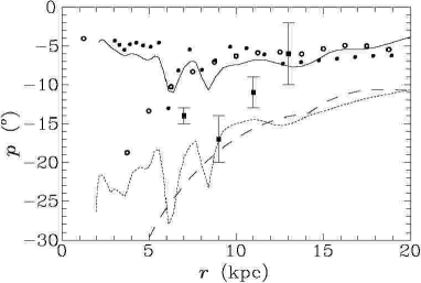
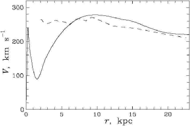
Figure 5: Left panel: The pitch angle of magnetic field in the galaxy M31 as obtained from radio polarization observations (squares with error bars) (Fletcher et al., 2004), from Eq. (33) using the rotation curve of Deharveng & Pellet (1975) and Haud (1981) (dashed) and Braun (1991) (dotted), and from Eq. (35) with $D_{\rm cr}=1$ using the same rotation curves (open and filled circles, respectively); $h(r)$ is twice the ${\rm H\,\scriptstyle I}$ scale height of Braun (1991). Results from a nonlinear dynamo model for M31 (Beck et al., 1998) are shown with solid line. Right panel: The rotation curve of M31 from Deharveng & Pellet (1975) and Haud (1981) (solid) and from Braun (1991) (dashed).

5 Observational evidence for the origin of
galactic magnetic fields

5.1 Magnetic pitch angle

Regular magnetic fields observed in spiral galaxies have field lines in the form of a spiral with a pitch angle in the range $p=-(10^{\circ}$–$30^{\circ})$, with negative values indicating a trailing spiral (e.g., Beck et al., 1996). As discussed in Sect. 4.1.4, the value of the pitch angle is a useful diagnostic of the mechanism maintaining the magnetic field.

Consider the simplest from of mean-field dynamo equations (10) and (11) appropriate for a thin galactic disc, but now written in terms of dimensional variables for $\overline{B}_{s}$ and $\overline{B}_{\phi}$:

$$\frac{\partial\overline{B}_{s}}{\partial t}=-\frac{\partial}{\partial z}(\alpha\overline{B}_{\phi})+\eta_{\rm T}\frac{\partial^{2}\overline{B}_{s}}{\partial z^{2}}\;,\qquad\frac{\partial\overline{B}_{\phi}}{\partial t}=G\overline{B}_{s}+\eta_{\rm T}\frac{\partial^{2}\overline{B}_{\phi}}{\partial z^{2}}\;.$$ (32)

Any regular magnetic field maintained by the dynamo must have a non-zero pitch angle: for $\overline{B}_{s}\equiv 0$ (a purely azimuthal magnetic field), equation for $\overline{B}_{\phi}$ in (32) reduces to a diffusion equation $\partial{\overline{B}}_{\phi}/\partial{t}=\eta_{\rm T}\partial^{2}\overline{B}_{\phi}/\partial{z^{2}}$ which only has decaying solutions, $\overline{B}_{\phi}\propto\mathrm{exp}(-\eta_{\rm T}t/h^{2})$. The same applies to a purely radial magnetic field.

Consider exponentially growing solutions, $\overline{B}_{s,\phi}={\cal B}_{s,\phi}\mathrm{exp}(\gamma t)$, and replace $\partial/\partial z$ by $1/h$ and $\partial^{2}/\partial z^{2}$ by $-1/h^{2}$ (as in the ‘no-$z$’ approximation) to obtain from Eqs. (32) two algebraic equations,

$$\left(\gamma+\eta_{\rm T}/h^{2}\right){\cal B}_{s}+\alpha{\cal B}_{\phi}/h=0\,,\quad-G{\cal B}_{s}+\left(\gamma+\eta_{\rm T}/h^{2}\right){\cal B}_{\phi}=0\,,$$

which have non-trivial solutions only if the determinant vanishes, which yields $(\gamma+\eta_{\rm T}/h^{2})^{2}\simeq-\alpha G/h$, and Eq. (25) follows with $D_{\rm cr}=1$. The resulting estimate of the magnetic pitch angle is given by

$$\tan p=\frac{{\cal B}_{s}}{{\cal B}_{\phi}}\approx-\sqrt{\frac{\alpha}{-Gh}}=-\sqrt{\frac{R_{\alpha}}{|R_{\omega}|}}\sim-\frac{\ell}{h}\left|\frac{\partial\ln\Omega}{\partial\ln s}\right|^{-1/2}\;.$$ (33)

For $\ell/h\simeq 1/4$ and a flat rotation curve, $\partial{\ln\Omega}/\partial{\ln s}=-1$, we obtain $p\simeq-15^{\circ}$, and this is the middle of the range observed in spiral galaxies. More elaborate treatments discussed by Ruzmaikin et al. (1988b) confirm this estimate of $p$ and yield a more accurate value of $D_{\rm cr}$. For example, the perturbation solution of Sect. 4.1.2 yields

$$p\approx-{\textstyle{\frac{1}{2}}}\pi^{3/2}\sqrt{\frac{R_{\alpha}}{|R_{\omega}|}}\;.$$ (34)

If the steady state is established by reducing $R_{\alpha}$ to its critical value as to obtain $R_{\alpha}R_{\omega}=D_{\rm cr}$, then the pitch angle in the nonlinear steady state becomes

$$\tan p\approx-{\textstyle{\frac{1}{2}}}\pi^{3/2}\frac{\sqrt{|D_{\rm cr}|}}{|R_{\omega}|}\;.$$ (35)

The magnetic pitch angle in M31 determined from observations and dynamo theory is shown in Fig. 5. Although the model curves show noticeable differences from the observed pitch angles, the general agreement is encouraging. The situation is typical: magnetic pitch angles of spiral galaxies are in a good agreement with predictions of dynamo theory (Beck et al., 1996).

This picture does not explain why the pitch angles of galactic magnetic fields are invariably close (though not equal) to those of the spiral pattern in the parent galaxy. A plausible explanation is that magnetic pitch angles are further affected by streaming motions associated with the spiral pattern to make the match almost perfect (Moss, 1998). We note, however, that the pitch angle of the large-scale magnetic field near the Sun differs significantly from that of the local (Orion) arm; it is not clear whether this misalignment is of a local or global nature.

As shown by Moss et al. (2000), magnetic pitch angle can be affected by an axisymmetric radial inflow (as well as outflow):

$$\tan p\approx-{\textstyle{\frac{1}{2}}}\pi^{3/2}\sqrt{\frac{R_{\alpha}}{|R_{\omega}|}}\left(1-{\textstyle{\frac{1}{2}}}{\cal R}\sqrt{\frac{\pi}{-D}}\,\right),\qquad{\cal R}=\frac{h^{2}}{2\eta_{\rm T}}\left(\frac{u_{s}}{s}-\frac{\partial u_{s}}{\partial s}\right),$$

which is useful to compare with Eqs (33) and (34). This effect is important if $u_{s}\;\raise 1.29167pt\hbox{$>$\kern-7.5pt\raise-4.73611pt\hbox{$\sim$}}\;\hskip-2.0pt2\eta_{\rm T}/h\linebreak[0]\simeq 1\,{\rm km\,s^{-1}}$ (cf. Sect. 5.5).

Twisting of a horizontal primordial magnetic field by galactic differential rotation leads to a tightly wound magnetic structure with magnetic field direction alternating with radius at a progressively smaller scale $\Delta s\sim s_{0}/|G|t$ with $\tan p\sim-(|G|t)^{-1}$, where $s_{0}\sim 10\,{\rm kpc}$ is the scale of variation in $\Omega$ (see §3.3 in Moffatt, 1978; Kulsrud, 1999 for a detailed discussion). The winding-up proceeds until a time $t_{0}\sim 5\times 10^{9}\,{\rm yr}$ such that $|G|t_{0}\sim|C_{\omega}|^{1/2},$ where $C_{\omega}=Gs_{0}^{2}/\eta_{\rm T}=R_{\omega}s_{0}^{2}/h^{2}\sim 10^{3}$–$10^{4}$. At later times, the alternating magnetic field rapidly decays because of diffusion and reconnection. The resulting maximum magnetic field strength achieved at $t_{0}$ is given by

$$B_{\rm max}\sim B_{0}|C_{\omega}|^{1/2}\;,$$ (36)

where $B_{0}$ is the external magnetic field; the magnetic field reverses at a small radial scale $\Delta s\sim s_{0}|C_{\omega}|^{-1/2}\sim 0.1\,{\rm kpc}$. The magnetic pitch angle at $t_{0}$ is of the order of $|p|\sim|C_{\omega}|^{-1/2}\;\raise 1.29167pt\hbox{$<$\kern-7.5pt\raise-4.73611pt\hbox{$\sim$}}\;\hskip-2.0pt1^{\circ}$, i.e., much smaller than the observed one. This picture cannot be reconciled with observations (cf. Kulsrud, 1999). It can be argued that streaming motions could make magnetic lines more open and parallel to the galactic spiral arms. However, then magnetic field will reverse on a small scale not only along radius, but also along azimuth. Such magnetic structures are quite different from what is observed. The moderate magnetic pitch angles observed in spiral galaxies are a direct indication that the regular magnetic field is not frozen into the interstellar gas and has to be maintained by the dynamo (Beck, 2000).

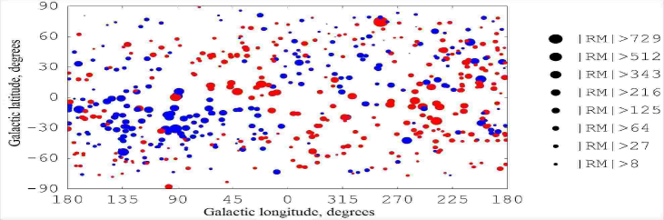
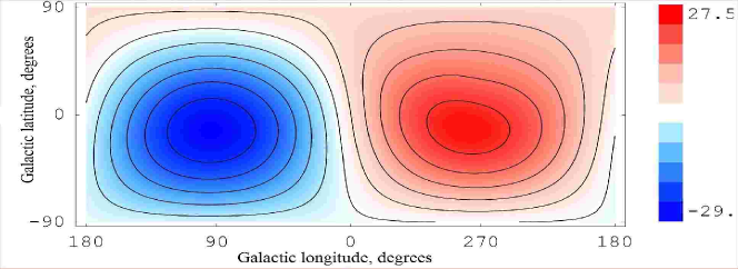
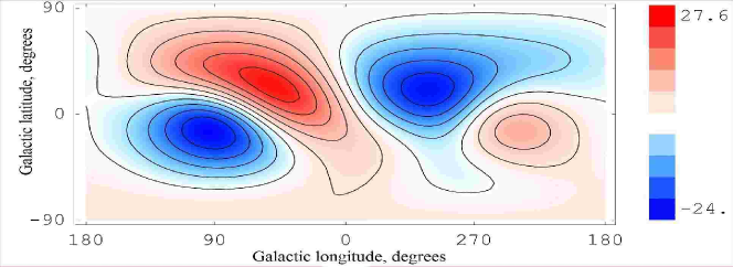
Figure 6: Upper panel: Faraday rotation measures of 551 extragalactic radio sources from the catalogue of Simard-Normandin & Kronberg (1980) shown in the $(l,b)$-plane, where $(l,b)$ are the Galactic longitude and latitude in a reference frame centred at the Sun with the Galactic center in the direction $l=0$ and Galactic midplane at $b=0$. Positive (negative) ${\rm RM}$s are shown with red (blue) circles whose radius indicates $|{\rm RM}|$ (rad m^-2) as shown to the right of the panel. The lower two panels show the wavelet transform of these data at scales $76^{\circ}$ (middle panel) and $35^{\circ}$ (lower panel) (Frick et al., 2001). The transform at $76^{\circ}$ has been obtained with the region of the Radio Loop I removed (this radio feature is a nearby supernova remnant). The wavelet transform at the scale $35^{\circ}$ is dominated by local magneto-ionic features.

5.2 The even (quadrupole) symmetry of magnetic field in the Milky Way

One of the most convincing arguments in favour of the galactic dynamo theory comes from the symmetry of the observed regular magnetic field with respect to the Galactic equator in the Milky Way. The direction of the magnetic field is determined from Faraday rotation measures of the cosmic sources of polarized emission, pulsars and extragalactic radio sources. Since the Galactic magnetic field has a significant random component and extragalactic radio sources can have their own (intrinsic) Faraday rotation, any meaningful conclusions about the Galactic magnetic field must rely on statistically significant samples of Faraday rotation measures. Even though the quadrupole symmetry of the galactic magnetic fields has been widely accepted as a firmly established fact since mid-1970’s, its objective observational verification has been obtained only recently. The main problem here is that it is difficult to separate local (small-scale) and global magnetic structures in the observed picture. However, wavelet analysis of the Faraday rotation measures of extragalactic radio sources has definitely confirmed that the horizontal components of the local regular magnetic field have even parity being similarly directed on both sides of the midplane (Frick et al., 2001, see Fig. 6).

The quadrupole symmetry is naturally explained by dynamo theory where even parity is strongly favoured against odd parity because the even field has twice larger scale in the vertical coordinate (see Sect. 4.1.2).

Primordial magnetic field twisted by differential rotation can have even vertical symmetry if it is parallel to the disc plane. However, then the field is rapidly destroyed by twisting and reconnection as described in Sect. 5.1. If, otherwise, the primordial field is parallel to the rotation axis and amplified by the vertical rotational shear $\partial\Omega/\partial z$ (which, however, is insignificant within galactic discs, $|z|\leq h$), it can avoid catastrophic decay (§3.11 in Moffatt, 1978), but then it will have odd parity in $z$, which is ruled out by the observed parity of the Milky Way field.

The derivation of the regular magnetic field of the Milky Way from Faraday rotation measures of pulsars and extragalactic radio sources, ${\rm RM}$, is complicated by the contribution of local magnetic perturbations, so it is difficult to decide which features of the RM sky are due to the regular magnetic field and which are produced by localized magneto-ionic perturbations (e.g., supernova remnants). Therefore, the same observational data have lead different authors to different conclusions (see Frick et al., 2001, for a recent review). Odd parity of the Galactic magnetic field has been suggested by Andreassian (1980, 1982) and, for the inner Galaxy, by Han et al. (1997). Quantitative methods of analysis (as opposed to the ‘naked-eye’ fitting of more or less arbitrarily selected models) are especially appropriate in this case.

Unfortunately, it is difficult to determine the parity of magnetic field in external galaxies. In galaxies seen edge-on, the disc is depolarized, whereas Faraday rotation in the halo is weak. Beck et al. (1994) found weak evidence of even magnetic parity in the lower halo of NGC 253. The arrangement of polarization planes in the halo of NGC 4631 (Beck, 2000) is very suggestive of odd parity, but this does not exclude even parity in the disc. In galaxies inclined to the line of sight, the amount of Faraday rotation produced by an odd (antisymmetric) magnetic field differs from zero because Faraday rotation and emission occur in the same volume; as a result, emission originating at the far half of the galactic layer will have small or zero net rotation, whereas emission from the near half will have significant rotation produced by the unidirectional magnetic field in that half. Therefore, Faraday rotation measures produced by even and odd magnetic structures of the same strength only differ by a factor of two (Krause et al., 1989a; Sokoloff et al., 1998) and it is difficult to distinguish between the two possibilities.

An interesting method to determine the parity of magnetic field in an external galaxy has been suggested by Han et al. (1998). These authors note that the contribution of the galaxy to the ${\rm RM}$ of a background radio source will be equal to the intrinsic ${\rm RM}$ of the galaxy if the magnetic field has even parity. For odd parity, the galaxy will not contribute to the ${\rm RM}$ of a background source, whereas any intrinsic ${\rm RM}$ will remain. The implementation of the method requires either a statistically significant sample of background sources or a single extended background source.

5.3 The azimuthal structure

Non-axisymmetric magnetic fields in a differentially rotating object are subject to twisting and enhanced dissipation as described in Sect. 5.1. The dynamo can compensate for the losses, but axisymmetric magnetic fields are still easier to maintain (Rädler, 1986). A few lowest non-axisymmetric modes with azimuthal wave numbers

$$m\;\raise 1.29167pt\hbox{$<$\kern-7.5pt\raise-4.73611pt\hbox{$\sim$}}\;\hskip-2.0pt\frac{s_{0}}{h}|R_{\omega}|^{-1/4}\approx 2$$ (37)

can be maintained in thin galactic disks where $h\ll s_{0}$ (§VII.8 in Ruzmaikin et al., 1988). The WKB solution of the galactic $\alpha\omega$-dynamo equations by Starchenko & Shukurov (1989) shows that the bisymmetric mode ($m=1$) can grow provided

$$\frac{u}{\ell\Omega}\left(\frac{h}{\ell}\right)^{2}\left|\frac{d\ln\Omega}{d\ln s}\right|\;\raise 1.29167pt\hbox{$<$\kern-7.5pt\raise-4.73611pt\hbox{$\sim$}}\;\hskip-2.0pt25\;,$$

which seems to be the case in some galaxies. These results indicate that it is natural to expect significant deviations from axial symmetry in magnetic fields of many spiral galaxies. However, the dominance of non-axisymmetric modes in most galaxies would be difficult to explain because the axisymmetric mode has the largest growth rate under typical conditions.

Early interpretations of Faraday rotation in spiral galaxies were in striking contrast with this picture, indicating strong dominance of bisymmetric magnetic structures $(m=1)$, ${\bf B}\propto\mathrm{exp}{(i\phi)}$ with $\phi$ the azimuthal angle (Sofue et al., 1986), and this was considered to be a severe difficulty of the dynamo theory and an evidence of the primordial origin of galactic magnetic fields. It was suggested by Ruzmaikin et al. (1986) (see also Sawa & Fujimoto, 1986; Baryshnikova et al., 1987) that the bisymmetric magnetic structures can be interpreted as the $m=1$ dynamo mode. However, despite effort, dynamo models could not explain the apparent widespread dominance of bisymmetric magnetic structures. Paradoxically, what seemed to be a difficulty of the dynamo theory has turned out to be its advantage as observations with better sensitivity and resolution and better interpretations have led to a dramatic revision of the observational picture. The present-day understanding is that modestly distorted axisymmetric magnetic structures occur in most galaxies, wherein the dominant axisymmetric mode is mixed with weaker higher azimuthal modes (Beck et al., 1996; Beck, 2000). Among nearby galaxies, only M81 remains a candidate for a dominant bisymmetric magnetic structure, but the data are old and this result needs to be reconsidered (Krause et al., 1989b); the interesting case of M51 is discussed below. Deviations from precise axial symmetry can result from the spiral pattern, asymmetry of the parent galaxy, etc. Dominant bisymmetric magnetic fields can be maintained by the dynamo action near the corotation radius due to a linear resonance with the spiral pattern (Mestel & Subramanian, 1991; Subramanian & Mestel, 1993; Moss, 1996) or nonlinear trapping of the field by the spiral pattern (Bykov et al., 1997).

Twisting of a horizontal magnetic field by differential rotation generally produces a bisymmetric magnetic field, $m=1$. Twisting of a horizontal primordial magnetic field can also produce an axisymmetric configuration near the galactic centre if the initial state is asymmetric (Sofue et al., 1986; Nordlund & Rögnvaldsson, 2002), with a maximum of the primordial field displaced from the disc’s rotation axis where the gas density is normally maximum. Thus, the maximum of the primordial field required by this scenario has to occur at a different position than the maximum in the gas density. This can only occur if the primordial field is not frozen into the gas — otherwise the field strength scales as a positive power of gas density. The fact that magnetic fields in most spiral galaxies are nearly axisymmetric within large radius (in fact, in the whole galaxy) would require that this strong asymmetry in the initial state occurs systematically for all the galaxies, which would be difficult to explain.

Figure 7: Left panels: The global magnetic structure of the galaxy M51, in the disc (upper left) and halo (bottom). Arrows show the direction and strength of the regular magnetic field on a polar grid shown superimposed on the optical image (Berkhuijsen et al., 1997). The grid radii are 3, 6, 9, 12 and 15 kpc. Upper right panel: Magnetic field strength from the dynamo model for the disc of M51 (Bykov et al., 1997) is shown with shades of grey (darker shade means stronger field). Magnetic field is reversed within the zero-level contour shown dashed; scale is given in kpc. The magnetic structure rotates rigidly together with the spiral pattern visible in the shades of grey.

5.4 A composite magnetic structure in M51 and magnetic reversals in the Milky Way

A striking example of a complicated magnetic structure that can hardly be explained by any mechanism other than the dynamo has been revealed in the galaxy M51 by Berkhuijsen et al. (1997). These authors used radio polarization observations of the galaxy at wavelengths 2.8, 6.2, 18.0 and $20.5\,{\rm cm}$ (smoothed to a resolution of $3.5\,{\rm kpc}$). The disc of this galaxy is not transparent to polarized radio emission at the two longer wavelengths. Therefore, it was possible to determine the magnetic field structure separately in two regions along the line the sight, which can be identified with the disc and halo of the galaxy. As shown in Fig. 7, the regular magnetic fields in the disc is reversed in a region about 3 by 8 kpc in size extended along azimuth at galactocentric radii $s=3$–6 kpc and azimuthal angles $300^{\circ}$–0 (shown with red arrows). A significant deviation from axial symmetry in the disc has been detected out to $s=9\,{\rm kpc}$ (in the azimuth range 160–$260^{\circ}$), although it is too weak to result in a magnetic field reversal. The field reversal occurs around the corotation radius in M51, $s\approx 6\,{\rm kpc}$ (i.e., the radius where the angular velocity of the spiral pattern is equal to that of the gas).

A nonlinear dynamo model for M51 was developed by Bykov et al. (1997) who used the rotation curve of M51, with the pitch angle of the spiral arms $-15^{\circ}$ and corotation radius 6 kpc. Figure 7 shows one of their solutions where a region with reversed magnetic field persists in the disc near the corotation radius of the spiral pattern. Near the corotation, a non-axisymmetric (bisymmetric) magnetic field can be trapped by the spiral pattern and maintained over the galactic lifetime. The effect is favoured by a smaller pitch angle of the spiral arms, thinner gaseous disc, weaker rotational shear and stronger spiral pattern. This nonaxisymmetric structure is arguably similar to the structure observed in M51.

The regular magnetic field in the halo of M51 has a structure very different from that in the disc — the halo field is nearly axisymmetric and even directed oppositely to that in the disc in most of the galaxy. An external magnetic field should have a rather peculiar form to be twisted into such a configuration!

Distinct azimuthal magnetic structures in the disc and the halo can be readily explained by dynamo theory as non-axisymmetric magnetic fields can be maintained only in the thin disc but not in the quasi-spherical halo where $h\simeq s_{0}$ and $|R_{\omega}|\gg 1$ in Eq. (37). Moreover, dynamo action in the disc and the halo can proceed almost independently of each other producing distinctly directed magnetic fields (Sokoloff & Shukurov, 1990).

Another case of a regular magnetic field with unusual structure is the Milky Way where magnetic field reversals are observed along the galactocentric radius in the inner Galaxy between the Orion and Sagittarius arms at $s\approx 7.9\,{\rm kpc}$ and, possibly, in the outer Galaxy between the Orion and Perseus arms at $s\approx 10.5\,{\rm kpc}$ (§3.8.2 in Beck et al., 1996, and Frick et al., 2001); see, however, Brown & Taylor 2001). The reversals were first interpreted as an indication of a global bisymmetric magnetic structure (Sofue & Fujimoto, 1983), but it has been shown that dynamo-generated axisymmetric magnetic field can have reversals at the appropriate scale (Ruzmaikin et al., 1985; Poezd et al., 1993). Both interpretations presume that the reversals are of a global nature, i.e., they extend over the whole Galaxy to all azimuthal angles (or radii in the case of the bisymmetric structure). This leads to a question why reversals at this radial scale are not observed in any other galaxy (Beck, 2000). Poezd et al. (1993) argue that the lifetime of the reversals is sensitive to subtle features of the rotation curve and the geometry of the ionized gas layer (see also Belyanin et al., 1994) and demonstrate that they are more probable to survive in the Milky Way than in, e.g., M31.

However, the observational evidence of the reversals is restricted to a relatively small neighbourhood of the Sun, of at most 3–5 kpc along azimuth. It is therefore quite possible that the reversals are local and arise from a magnetic structure similar to that in the disc of M51 as shown in Fig. 7. The reversed field in the Solar neighbourhood has the same radial extent of 2–3 kpc as in M51 and also occurs near the corotation radius. This possibility has not yet been explored; its observational verification would require careful analysis of pulsar Faraday rotation measures.

5.5 The radial magnetic structure in M31

An important clue to the origin of galactic magnetic field is provided by the magnetic ring in M31 (Beck, 1982), predicted by dynamo theory (Ruzmaikin & Shukurov, 1981). Both the large-scale magnetic field and the gas density in this galaxy have a maximum in the same annulus $8\;\raise 1.29167pt\hbox{$<$\kern-7.5pt\raise-4.73611pt\hbox{$\sim$}}\;\hskip-2.0pts\;\raise 1.29167pt\hbox{$<$\kern-7.5pt\raise-4.73611pt\hbox{$\sim$}}\;\hskip-2.0pt12\,{\rm kpc}$, with the apparent enhancement in the magnetic field strength by about 30% (Fletcher et al., 2004). The kinematic dynamo model of Ruzmaikin & Shukurov (1981) was based on the double-peaked rotation curve of shown in Fig. 5, where rotational shear is strongly reduced at $s=2$–6 kpc. As a result, $R_{\omega}$ is small and even positive in this radial range, so $|D|<|D_{\mathrm{cr}}|$ and the dynamo cannot maintain any regular magnetic field at $s=2$–6 kpc.

An attractive aspect of this theory is that both magnetic and gas rings are attributed to the same feature of the rotation curve. Angular momentum transport by viscous stress leads to matter inflow at a rate $\dot{M}=2\pi\Sigma\nu_{\rm T}\partial{\ln\Omega}/\partial{\ln s}\sim 0.1\,M_{\odot}\,{\rm yr}^{-1}$, where $\nu_{\rm T}\sim\eta_{\rm T}$ is the turbulent viscosity, resulting in the radial inflow at a speed $u_{s}=\dot{M}/2\pi s\Sigma$ with $\Sigma$ the gas surface density. In the nearly-rigidly rotating parts, $u_{s}$ is reduced and matter piles up outside this region producing gas ring. Gravitational torques from spiral arms can further enhance the inflow (see Moss et al., 2000, for a discussion), so the total radial velocity is expected to be $u_{s}\sim 1\,{\rm km\,s^{-1}}$ at $s=10\,{\rm kpc}$.

The double-peaked rotation curve of M31 is consistent with the existence of both magnetic and gas rings. The situation is different with the more recent rotation curve of Braun (1991) which does not have a double-peaked shape (Fig. 5). The difference between the two rotation curves arises mainly from the fact that Braun allows for significant displacements of spiral arm segments from the galactic midplane: this results in a revision of the segments’ galactocentric distances for regions away from the major axis. We note that the CO velocity field at the major axis (Loinard et al., 1995) is compatible with a double-peaked rotation curve.

With Braun’s rotation curve, the magnetic field can concentrate into a ring mainly because the gas is in the ring and $B\propto\rho^{1/2}$ as shown in Eq. (4.1.5). The dynamo model of Moss et al. (1998) based on the rotation curve of Braun (1991) has difficulties in reproducing a magnetic ring as well pronounced as implied by the observed amount of Faraday rotation. This has lead to an idea that magnetic field can be significant at $s=2$–$6\,{\rm kpc}$ in M31. This has prompted Han et al. (1998) to search for magnetic fields at $s=2$–6 kpc that could have escaped detection because of reduced density of cosmic ray electrons at those radii. These authors have found that two out of three background polarized radio sources seen through that region of M31 have Faraday rotation measures compatible with the results of Moss et al. (1998). They further conclude that this indicates an even symmetry of the regular magnetic field. This is encouraging, but a statistically representative sample of background sources has to be used to reach definite conclusions because of their unknown intrinsic ${\rm RM}$.

With a double-peaked rotation curve, a primordial magnetic field with a uniform radial component could have been twisted to produce a magnetic ring by virtue of Eq. (36). In this case the primordial and dynamo theories have similar problems and possibilities regarding the magnetic ring in M31.

Lou & Fan (2000) attribute the magnetic ring in M31 to an axisymmetric mode of MHD density waves. Because of the axial symmetry of the wave, the magnetic field in the ring must be purely azimuthal, $p=0$, in contrast to the observed structure with a significant pitch angle (Fig. 5). Furthermore, the ring can hardly represent a wave packet as envisaged in this theory because then its group velocity must be comparable to the Alfvén speed of $30\,{\rm km\,s^{-1}}$ (Lou & Fan, 1998) and so the ring should be travelling at this speed along radius to traverse 30 kpc in $10^{9}\,{\rm yr}$, a distance much larger than the ring radius. The implication would be that the ring is a transient with a short lifetime of order $3\times 10^{8}\,{\rm yr}$. And, of course, the theory cannot explain the origin of an azimuthal magnetic field required to launch the wave packet.

5.6 Strength of the regular magnetic field

Interstellar regular magnetic fields are observed to be close to the energy equipartition with interstellar turbulence. This directly indicates that the regular magnetic field is coupled to the turbulent gas motions. (Note that $\ell\Omega$ does not differ much from the turbulent velocity $u_{0}$ in Eq. (4.1.5).) To appreciate the importance of this conclusion, consider primordial magnetic field twisted by differential rotation. Its maximum strength given by Eq. (36) as $B_{\rm max}\sim 10^{2}B_{0}$ is controlled by the strength of the primordial field $B_{0}$, and so this theory, if applicable, would result in stringent constraints on extragalactic magnetic fields.

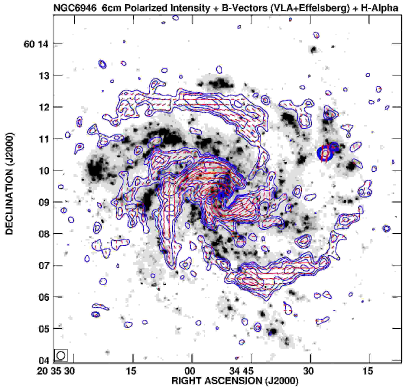
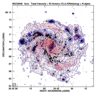
Figure 8: Left panel: Magnetic arms in the galaxy NGC 6946: polarized intensity at the wavelength $\lambda=6\,{\rm cm}$ (blue contours), a tracer of the large-scale magnetic field $\overline{B}$, superimposed on the galactic image in the H$\alpha$ spectral line of ionized hydrogen (grey scale). Red dashes indicate the orientation of the $E$-vector of the polarized emission (parallel to the direction of intrinsic magnetic field if Faraday rotation is negligible), with length proportional to the fractional polarization — see Eq. (5). The spiral arms visualized by H$\alpha$ are the sites where gas density is maximum. The large-scale magnetic field is evidently stronger between the arms where gas density is lower. Right panel: As in the left panel, but now for the total synchrotron intensity, a tracer of the total magnetic field $B^{2}=\overline{B}^{2}+\overline{b^{2}}$. The total field is enhanced in the gaseous arms. Given that the large-scale field concentrates between the arms, this means that the random field is significantly stronger in the arms, a distribution very different from that of the large-scale field. The size of the beam in the radio maps is shown in the bottom left of each frame. (Images courtesy of R. Beck, MPIfR, Bonn.)

A striking evidence of the nontrivial behaviour of the large-scale galactic magnetic field is the so-called magnetic arms, first discovered by Beck & Hoernes (1996) in the nearby galaxy NGC 6946. We show in Fig. 8 a map of polarized radio emission from this galaxy (a tracer of the large-scale magnetic field strength) superimposed on the map in the H$\alpha$ spectral line (a tracer of ionized gas). It is evident that magnetic field is stronger between the spiral arms of this galaxy, i.e., where the gas density (both total and ionized) is lower. This behaviour is just opposite to what is expected of a frozen-in magnetic field that scales with a power of gas density. The phenomenon of magnetic arms confirms in a spectacular manner that the large-scale magnetic field is not frozen into the interstellar gas, and therefore cannot be primordial. Shukurov (1998), Moss (1998) and Rohde et al. (1999) suggest an explanation of the magnetic arms in terms of the mean-field dynamo theory. In brief, they argue that dynamo number can be larger between the gaseous spiral arms, resulting in stronger dynamo action.

The theory of MHD density waves relates magnetic field excess $\Delta\overline{B}$ in spiral arms to the enhancement in stellar density, $\Delta\overline{B}/\langle\overline{B}\rangle=\Delta\Sigma/\langle\Sigma\rangle$ (Lou & Fan, 1998), where $\Sigma$ is the stellar surface density, $\Delta\Sigma$ is its excess in the spiral arms, and angular brackets denote azimuthal averaging. Arm intensities in magnetic field and stellar surface density in NGC 6946 have been estimated by Frick et al. (2000) who applied wavelet transform techniques to radio polarization maps and to the galaxy image in broadband red light, a tracer of stellar mass density. Their results indicate that the mean relative intensity of magnetic spiral arms remains rather constant with galactocentric radius at a level of 0.3–0.6. On the contrary, the relative strength of the stellar arms systematically grows with radius from very small values in the inner galaxy to 0.3–0.7 at $s=5$–6 kpc, and then decreases to remain at a level of 0.1–0.3 out to $s=12\,{\rm kpc}$. The distinct magnitudes and radial trends in the strengths of magnetic and stellar arms in NGC 6946 do not seem to support the idea that the magnetic arms are due to MHD density waves.

6 Elliptical galaxies

Elliptical galaxies do not rotate fast enough, so they are ellipsoidal systems without prominent disc components. The stellar population of elliptical galaxies is old and the interstellar gas is dilute (Mathews & Brighenti, 2003). Therefore, both relativistic and thermal electrons have low density, and any synchrotron emission and Faraday rotation can only be weak. Nevertheless, there are several lines of evidence, albeit mostly indirect, suggesting significant magnetic fields in ellipticals (Moss & Shukurov, 1996; Mathews & Brighenti, 1997). The magnetic field should be random, producing unpolarized synchrotron emission and fluctuating Faraday rotation. The r.m.s. Faraday rotation measure attributable to the ISM of the ellipticals is $\langle\mbox{RM}\rangle=5$–100 rad m^-2.

6.1 Turbulent interstellar gas in elliptical galaxies

Interstellar gas in elliptical galaxies is observed via its X-ray emission. Type I supernovae (SNe) (and also stellar winds and random motions of stars) heat the gas to the observed temperatures $T\simeq 10^{7}\,{\rm K}$. It is natural to expect that a fraction $\delta$ of the energy is converted into turbulent motions of the gas. The turbulent scale $\ell\approx 400\,$pc is given by the diameter of a SN as it reaches pressure balance with the ambient medium whose typical density is $n\approx 10^{-3}\,{\rm cm^{-3}}$. The balance between energy injection and dissipation rates yields a turbulent velocity of $u_{0}\simeq 20\,{\rm km\,s^{-1}}$ for $\delta=0.1$, assuming the energy dissipation time $\tau\simeq\ell/u_{0}$ as for the Kolmogorov turbulence. This estimate of $u_{0}$ is compatible with the constraint $u_{0}\;\raise 1.29167pt\hbox{$<$\kern-7.5pt\raise-4.73611pt\hbox{$\sim$}}\;\hskip-2.0pt50\,{\rm km\,s^{-1}}$ resulting from the observed X-ray luminosity. Another driver of turbulence is the random motions of stars. These generate random vortical motions at a smaller scale and velocity, $\ell_{*}\simeq 3\,{\rm pc}$ and $u_{*}\simeq 3\,{\rm km\,s^{-1}}$, respectively (Moss & Shukurov, 1996).

The driving force produced by an expanding quasi-spherical SN remnant is potential. The above estimates assume that the motions driven by the SNe are vortical, so $\tau=\ell/u_{0}$ applies. In spiral galaxies, the potential (acoustic) motions are efficiently converted into vortical turbulence mainly due to the inhomogeneity of the ISM. The ISM in elliptical galaxies is hot and, presumably, rather homogeneous at kpc scales. Therefore, Moss & Shukurov (1996) suggested that SNe will drive sound-wave turbulence whose correlation time $\tau$ is $(u_{0}/c_{\mathrm{s}})^{-2}\ell/c_{\mathrm{s}}\sim 3\times 10^{7}\,{\rm yr}$ rather than $\ell/u_{0}$, where $c_{\mathrm{s}}\approx 300\,{\rm km\,s^{-1}}$ is the speed of sound. However, Mathews & Brighenti (1997) noted that sound waves quickly dissipate, and so cannot form a pervasive turbulent velocity field. The nature of turbulence in elliptical galaxies needs to be studied further.

6.2 The fluctuation dynamo in elliptical galaxies

As in most astrophysical objects, Rm in elliptical galaxies by far exceeds 100, so fluctuation dynamo action in ellipticals is quite plausible (see Sect. 4.2). The e-folding time of the random field in a vortical random flow is of the order of the eddy turnover time, $\tau=2\times 10^{7}\,{\rm yr}$. The magnetic field is concentrated into flux ropes whose length and thickness are of order $\ell\simeq 400\,$pc and $\ell\mbox{Rm}_{\mathrm{cr}}^{-1/2}\simeq 40\,{\rm pc}$. In the ropes, magnetic field is plausibly in equipartition with the turbulent kinetic energy, $b\simeq 0.3\,\mu{\rm G}$.

Moss & Shukurov (1996) discuss a two-stage dynamo action by smaller scale vortical turbulence driven by random motions of the stars and, at larger scales, by the acoustic turbulence. However, the very existence of the acoustic turbulence in elliptical galaxies is questionable (Mathews & Brighenti, 1997).

Faraday rotation measure produced within a single turbulent cell with the above parameters is ${\rm RM}_{0}\simeq 0.81bn_{\rm e}\ell$, so the net Faraday rotation from an ensemble of turbulent cells, observed at a resolution $D$ such that $D\gg\ell$, is given by $\langle{\rm RM}\rangle\sim{\rm RM}_{0}\sqrt{{N}/{N_{D}}}\sim{\rm RM}_{0}{\sqrt{L\ell}}/{D}\,,$ where $N=L/\ell$ is the number of cells along the path length $L$ and $N_{D}=(D/\ell)^{2}$ is the number of cells in the resolution element. Thus, ${\rm RM}_{0}\simeq 0.1\,{\rm rad\,m^{-2}}$ and $\langle{\rm RM}\rangle\sim 1\,{\rm rad\,m^{-2}}$. Faraday rotation can be stronger in the central regions where $\langle{\rm RM}\rangle\sim 5\,{\rm rad\,m^{-2}}$ at a distance 8 kpc from the galactic centre. These estimates agree fairly with the available observations.

Magnetic field generation in elliptical galaxies was discussed by Lesch & Bender (1990), but they considered a mean-field dynamo that needs overall rotation which is not present in elliptical galaxies. The fluctuation dynamo in elliptical (radio) galaxies was simulated by De Young (1980), but these simulations apparently had $\mbox{Rm}<\mbox{Rm}_{\mathrm{cr}}$ as they resemble transient amplification of magnetic field by velocity shear rather than genuine dynamo action.

7 Conclusions

The observational picture of galactic magnetic fields is compatible with the mean-field dynamo theory in its simplest, quasi-kinematic form. It is important to note that there is not much freedom in varying parameters of galactic dynamos as observations constrain them fairly tightly. Therefore, this agreement is not a result of a free-hand parameter adjustments. Moreover, galactic dynamo theory has demonstrated its predictive power. For example, it has been clear to dynamo theorists since the early 1970’s that the partially ionized Galactic disc has the scale height 0.4–0.5 kpc, i.e., significantly larger than that of the neutral hydrogen layer (see §VI.2 in Ruzmaikin et al., 1988, for a review), but the existence of this component of the interstellar medium was accepted by a broader astrophysical community only 15 years later (Lockman, 1984).

The agreement of the mean-field dynamo theory with observations discussed in Sect. 5 cannot be considered as a proof of its correctness — history of physics is familiar with concepts, such as the ether, that have proved to be irrelevant despite their perfect agreement with numerous experimental facts, before a single experiment refuted them. Nevertheless, the spectacular success of the dynamo theory when applied to galaxies warrants its careful treatment when compared with other theories. In particular, any rival theory has to be able to explain at least the same set of observational data as the dynamo theory. In this sense, there are no fair rivals to the dynamo theory.

The main current difficulty of the galactic dynamo theory is our lack of understanding of its nonlinear form. It is important to avoid an unjustified extension to real galaxies of results obtained for highly idealized systems. In particular, the disc of a spiral galaxy is not a closed system. The significance of the disc-halo connection for the mean-field galactic dynamos, touched upon in Sect. 4.3, should be carefully investigated.

Another outstanding problem in theory and observations of galactic magnetic fields is the effect of the multi-phase structure of the interstellar medium on the magnetic field. The effect of magnetic fields on the multi-phase structure is also expected to be very significant, and also poorly understood. The strength of the magnetic field in the hot phase is not known. The detailed nature of the balance between cosmic rays and magnetic field has to be clarified: it is unclear whether this balance is maintained pointwise (at each location) or only on average (e.g., at scales exceeding the diffusion scale of cosmic ray particles). The answer to this question is essential for the interpretation of the synchrotron emission from spiral galaxies. Progress in this direction will eventually make theory of galactic magnetic fields an integral part of galactic astrophysics.

References

Andreassian R. R., On the structure of the Galactic magnetic field. Astrofizika, 16, 707–713 (1980).

Andreassian R. R., A study of the magnetic field of the Galaxy. Astrofizika, 18, 255–262 (1982).

Armstrong J. W., Rickett B. J. & Spangler S. R., Electron density power spectrum in the local interstellar medium. Astrophys. J., 443, 209–221 (1995).

Baryshnikova Yu., Ruzmaikin A., Sokoloff D. & Shukurov A., Generation of large-scale magnetic fields in spiral galaxies. Astron. Astrophys., 177, 27–41 (1987).

Beck R., The magnetic field in M31. Astron. Astrophys., 106, 121–132 (1982).

Beck R., Magnetic fields and interstellar gas clouds in the spiral galaxy NGC 6946. Astron. Astrophys., 251, 15–26 (1991). Erratum: Astron. Astrophys., 258, 605 (1992).

Beck R., Magnetic fields in normal galaxies. Phil. Trans. R. Soc. Lond., A358, 777–796 (2000).

Beck R., Galactic and extragalactic magnetic fields. Sp. Sci. Rev., 99, 243–260 (2001).

Beck R. & Hoernes P., Magnetic spiral arms in the galaxy NGC 6946. Nature, 379, 47–49 (1996).

Beck R., Carilli C. L., Holdaway M. A. & Klein U., Multifrequency observations of the radio continuum emission from NGC 253. I. Magnetic fields and rotation measures in the bar and halo. Astron. Astrophys., 292, 409–424 (1994).

Beck R., Brandenburg A., Moss D., Shukurov A. & Sokoloff D., Galactic magnetism: recent developments and perspectives. Ann. Rev. Astron. Astrophys., 34, 155–206 (1996).

Beck R., Berkhuijsen E. M., Moss D., Shukurov A. & Sokoloff D., The nature of the magnetic belt in M31. Astron. Astrophys., 335, 500–509 (1998).

Beck R., Shukurov A., Sokoloff D. & Wielebinski R., Systematic bias in interstellar magnetic field estimates. Astron. Astrophys., 411, 99–107 (2003) (astro-ph/0307330).

Belyanin M., Sokoloff D., Shukurov A., Simple models of nonlinear fluctuation dynamo. Geophys. Astrophys. Fluid Dyn., 68, 237–261 (1993).

Belyanin M. P., Sokoloff D. D. & Shukurov A. M., Asymptotic steady-state solutions to the nonlinear hydromagnetic dynamo equations. Russ. J. Math. Phys., 2, 149–174 (1994).

Berkhuijsen E. M., Horellou C., Krause M., Neininger N., Poezd A. D., Shukurov A. & Sokoloff D. D., Magnetic fields in the disk and halo of M51. Astron. Astrophys., 318, 700–720 (1997).

Blackman, E. G., & Field, G. B., Coronal activity from dynamos in astrophysical rotators. Mon. Not. R. Astron. Soc., 318, 724–732 (2000).

Boulares A. & Cox D. P., Galactic hydrostatic equilibrium with magnetic tension and cosmic-ray diffusion. Astrophys. J., 365, 544–558 (1990).

Brandenburg A. & Subramanian K., Astrophysical magnetic fields and nonlinear dynamo theory. Phys. Rep., in press (2004).

Brandenburg A., Donner K.-J., Moss D., Shukurov, A., Sokoloff D. D. & Tuominen I., Dynamos in discs and halos of galaxies. Astron. Astrophys., 259, 453–461 (1992).

Brandenburg A., Donner K.-J., Moss D., Shukurov, A., Sokoloff D. D. & Tuominen I., Vertical magnetic fields above the discs of spiral galaxies. Astron. Astrophys., 271, 26–50 (1993).

Brandenburg A., Moss D. & Shukurov A., Galactic fountains as magnetic pumps. Mon. Not. R. Astron. Soc., 276, 651–662 (1995).

Brandenburg, A., Dobler, W. & Subramanian, K., Magnetic helicity in stellar dynamos: new numerical experiments. Astron. Nachr., 323, 99–122 (2002).

Braun R., The distribution and kinematics of neutral gas in M31. Astrophys. J., 372, 54–66 (1991).

Brown J. C. & Taylor A. R., The structure of the magnetic field in the outer galaxy from rotation measure observations through the disk. Astrophys. J. Lett., 563, L31–L34 (2001).

Bykov A., Popov V., Shukurov A., Sokoloff D., Anomalous persistence of bisymmetric magnetic structures in spiral galaxies. Mon. Not. R. Astron. Soc., 292, 1–10 (1997).

Cattaneo F., Hughes D. W. & Kim, E.-J., Suppression of chaos in a simplified nonlinear dynamo model. Phys. Rev. Lett., 76, 2057–2060 (1996).

Clemens D. P., Massachusetts–Stony Brook Galactic plane CO survey: the Galactic disk rotation curve. Astrophys. J., 295, 422–436 (1985).

Cox D. P., The diffuse interstellar medium. In The Interstellar Medium in Galaxies, eds H. A. Thronson & J. M. Shull, Kluwer, Dordrecht, pp. 181–200 (1990).

Deharveng J. M. & Pellet A., Étude cinématique et dynamique de M31 à partir de l’observation des régions d’émission. Astron. Astrophys., 38, 15–28 (1975).

De Young D., Turbulent generation of magnetic fields in extragalactic radio sources. Astrophys. J., 241, 81–97 (1980).

Dopita M. A. & Sutherland R. S., Astrophysics of the Diffuse Universe, Springer, Berlin (2003).

Elstner D., Meinel R. & Rüdiger G., Galactic dynamo models without sharp boundaries. Geophys. Astrophys. Fluid Dyn., 50, 85–94 (1990).

Elstner D., Golla G., Rüdiger G. & Wielebinski R., Galactic halo magnetic fields due to a ‘spiky’ wind. Astron. Astrophys., 297, 77–82 (1995).

Fletcher A. & Shukurov A., Hydrostatic equilibrium in a magnetized, warped Galactic disc. Mon. Not. R. Astron. Soc., 325, 312–320 (2001).

Fletcher A., Berkhuijsen E. M., Beck R. & Shukurov A., The magnetic field of M31 from multi-wavelength radio polarization observations, Astron. Astrophys., in press (2004) (astro-ph/0310258).

Fraternali F., Oosterloo T., Boomsma R., Swaters R. & Sancisi R., High velocity gas in the halos of spiral galaxies. In Recycling Intergalactic and Interstellar Matter, IAU Symp. 217, eds P.-A. Duc, J. Braine & E. Brinks, ASP (2003) (astro-ph/0310799).

Frick P., Beck R., Shukurov A., Sokoloff D., Ehle M., Kamphuis J., Radio and optical spiral patterns in the galaxy NGC 6946. Mon. Not. R. Astron. Soc., 318, 925–937 (2000).

Frick P., Stepanov R., Shukurov A., Sokoloff D., Structures in the rotation measure sky. Mon. Not. R. Astron. Soc., 325, 649–664 (2001) (astro-ph/0012459).

Han J. L., Manchester R. N., Berkhuijsen E. M. & Beck R., Antisymmetric rotation measures in our Galaxy: evidence for an A0 dynamo. Astron. Astrophys., 322, 98–102 (1997).

Han J. L., Beck R. & Berkhuijsen E. M., New clues to the magnetic field structure of M31. Astron. Astrophys., 335, 1117–1123 (1998).

Haud U., Gas kinematics in M31. Astrophys. Space Sci., 76, 477–490 (1981).

Kahn F. D., Brett L., Magnetic reconnection in the disc and halo. Mon. Not. R. Astron. Soc., 263, 37–48 (1993).

Kazantsev A. P., Enhancement of a magnetic field by a conducting fluid. Zh. Teor. Eksper. Fiz., 53, 1806–1813 (1967); English translation: Sov. Phys. JETP, 26, 1031–1034 (1968).

Kazantsev A. P., Ruzmaikin A. A. & Sokoloff D. D., Magnetic field transport in an acoustic turbulence. Sov. Phys. JETP, 61, 285–292 (1985).

Kleeorin N., Moss D., Rogachevskii I. & Sokoloff D., Helicity balance and steady-state strength of the dynamo generated galactic magnetic field. Astron. Astrophys., 361, L5–L8 (2000).

Kleeorin N., Moss D., Rogachevskii I. & Sokoloff D., Nonlinear magnetic diffusion and magnetic helicity transport in galactic dynamos. Astron. Astrophys., 400, 9–18 (2003).

Korpi M. J., Brandenburg A., Shukurov A., Tuominen I. & Nordlund Å., A supernova-regulated interstellar medium: simulations of the turbulent multiphase medium. Astrophys. J. Lett., 514, L99–L102 (1999a).

Korpi M. J., Brandenburg A., Shukurov A. & Tuominen I., Evolution of a superbubble in a turbulent, multi-phased and magnetized ISM. Astron. Astrophys., 350, 230–239 (1999b).

Krasheninnikova Yu. S., Ruzmaikin A. A,, Sokoloff D. D. & Shukurov A., Configuration of large-scale magnetic fields in spiral galaxies. Astron. Astrophys., 213, 19–28 (1989).

Krause M., Beck R. & Hummel E., The magnetic field structures in two nearby spiral galaxies. I. The axisymmetric spiral magnetic field in IC342. Astron. Astrophys., 217, 1–17 (1989a).

Krause M., Beck R. & Hummel E., The magnetic field structures in two nearby spiral galaxies. II. The bisymmetric spiral magnetic field in M81. Astron. Astrophys., 217, 17–30 (1989b).

Kvasz L., Sokoloff D. D. & Shukurov A., A steady state of the disk dynamo. Geophys. Astrophys. Fluid Dyn., 65, 231–244 (1992).

Kulsrud R. M., A critical review of galactic dynamos. Ann. Rev. Astron. Astrophys., 37, 37–64 (1999).

Kulsrud R. M., Cen R., Ostriker J. P. & Ryu D., The protogalactic origin for cosmic magnetic fields. Astrophys. J., 480, 481–491 (1997).

Lesch H. & Bender R., Magnetic fields in elliptical galaxies. Astron. Astrophys., 233, 417–421 (1990).

Lockman F. J., The ${\rm H\,\scriptstyle I}$ halo in the inner galaxy. Astrophys. J., 283, 90–97 (1984).

Loinard L., Allen R. J., Lequeux J., An unbiased survey for CO emission in the inner disk of the Andromeda galaxy. Astron. Astrophys., 301, 68–74 (1995).

Lou Y.-Q., Fan A., Coupled galactic density-wave modes in a composite system of thin stellar and gaseous discs. Mon. Not. R. Astron. Soc., 297, 84–100 (1998).

Lou Y.-Q., Fan A., Large-scale magnetohydrodynamic density-wave structures in the Andromeda nebula. Mon. Not. R. Astron. Soc., 315, 646–654 (2000).

Lozinskaya T. A., Supernovae and Stellar Winds in the Interstellar Medium, AIP, New York (1992).

Mathews W. G. & Brighenti F., Self-generated magnetic fields in galactic cooling flows . Astrophys. J., 488, 595–605 (1997).

Mathews W. G. & Brighenti F., Hot gas in and around elliptical galaxies. Ann. Rev. Astron. Astrophys., 41, 191–239 (2003).

Mestel L. & Subramanian K., Galactic dynamos and density wave theory. Mon. Not. R. Astron. Soc., 248, 677–687 (1991).

McKee C. F. & Ostriker J. P., A theory of the interstellar medium: three components regulated by supernova explosions in inhomogeneous substrate. Astrophys. J., 217, 148–169 (1977).

Moffatt H. K., Magnetic Field Generation in Electrically Conducting Fluids, Cambridge Univ. Press (1978).

Moss D., On the generation of bisymmetric magnetic-field structures in spiral galaxies by tidal interactions. Mon. Not. R. Astron. Soc., 275, 191–194 (1995).

Moss D., Parametric resonance and bisymmetric dynamo solutions in spiral galaxies. Astron. Astrophys., 308, 381–386 (1996).

Moss D., The relation between magnetic and gas arms in spiral galaxies. Mon. Not. R. Astron. Soc., 297, 860–866 (1998).

Moss D. & Shukurov A., Turbulence and magnetic fields in elliptical galaxies. Mon. Not. R. Astron. Soc., 279, 229–239 (1996).

Moss D. & and Shukurov A., Galactic dynamos with captured magnetic flux and an accretion flow. Astron. Astrophys., 372, 1048–1063 (2001) (astro-ph/0012436).

Moss D. & and Shukurov A., Accretion disc dynamos opened up by external magnetic fields, Astron. Astrophys., 413, 403–414 (2004).

Moss D., Shukurov A. & Sokoloff D., Galactic dynamos driven by magnetic buoyancy. Astron. Astrophys., 343, 120–131 (1999).

Moss D., Shukurov A. & Sokoloff D., Accretion and galactic dynamos. Astron. Astrophys., 358, 1142–1150 (2000).

Moss D., Shukurov A., Sokoloff D., Beck R. & Fletcher A., Magnetic fields in barred galaxies. II. Dynamo models. Astron. Astrophys., 380, 55–71 (2001) (astro-ph/0107214).

Niklas S., Eigenschaften von Spiralgalaxien in hochfrequenten Radiokontinuum. PhD Thesis, Max-Planck-Institut für Radioastronomie, Bonn (1995).

Nordlund Å. & Rögnvaldsson Ö., Magnetic fields in young galaxies. Highlights Astron., 12, 706–708 (2002).

Parker E. N., The generation of magnetic fields in astrophysical bodies. II. The galactic field. Astrophys. J., 163, 252–278 (1971).

Phillips A., A comparison of the asymptotic and no-$z$ approximations for galactic dynamos. Geophys. Astrophys. Fluid Dyn., 94, 135–150 (2001).

Poezd A., Shukurov A. & Sokoloff D., Global magnetic patterns in the Milky Way and the Andromeda nebula. Mon. Not. R. Astron. Soc., 264, 285–297 (1993).

Priklonsky V., Shukurov A., Sokoloff D. & Soward A., Non-local effects in the mean-field disc dynamo. I. An asymptotic expansion. Geophys. Astrophys. Fluid Dyn., 93, 97–114 (2000) (astro-ph /0309666).

Rädler K.-H., On the effect of differential rotation on axisymmetric and non-axisymmetric magnetic fields of cosmical bodies. In Plasma Astrophysics, ESA Publ. SP-251, pp. 569–574 (1986).

Rohde R., Beck R. & Elstner D., Magnetic arms in NGC 6946 generated by a turbulent dynamo. Astron. Astrophys., 350, 423–433 (1999).

Ruzmaikin A. A. & Shukurov A. M., Magnetic field generation in the Galactic disk. Sov. Astron., 25, 553–558 (1981).

Ruzmaikin A. A., Sokoloff D. D. & Shukurov A. M., Magnetic field distribution in spiral galaxies. Astron. Astrophys., 148, 335–343 (1985).

Ruzmaikin A. A., Sokoloff D. D. & Shukurov A. M., Magnetic fields in spiral galaxies. In Plasma Astrophysics, ESA Publ. SP-251, pp. 539–544 (1986).

Ruzmaikin A. A., Shukurov A. M. & Sokoloff D. D., Magnetic Fields of Galaxies, Kluwer, Dordrecht (1988).

Sawa T. & Fujimoto M., Bisymmetric spiral configuration of magnetic fields in spiral galaxies. I. Local theory. Publ. Astron. Soc. Japan, 38, 551–566 (1986).

Schekochikhin A., Cowley S., Hamnett G.W., Maron J. L. & McWilliams J. C., A model of nonlinear evolution and saturation of the turbulent MHD dynamo. New J. Phys., 4, 84.1–84.22 (2002) (astro-ph/0207503).

Segalovitz A., Shane W. W., de Bruyn A. G., Polarisation detection at radio wavelengths in three spiral galaxies, Nature, 264, 222–226 (1976).

Shapiro P. R. & Field G. B., Consequences of a new hot component of the interstellar medium. Astrophys. J., 205, 762–765 (1976).

Shukurov A., Magnetic spiral arms in galaxies. Mon. Not. R. Astron. Soc., 299, L21–L24 (1998).

Shukurov A. & Berkhuijsen E. M., Faraday ghosts: depolarization canals in the Galactic radio emission. Mon. Not. R. Astron. Soc., 342, 496–500 (2003). Erratum: Mon. Not. R. Astron. Soc., 345, 1392 (2003) (astro-ph/0303087).

Shukurov A. & Sokoloff D., Galactic spiral arms and dynamo control parameters. Studia Geoph. et Geod., 42, 391–396 (1998).

Shukurov A., Sarson G. R., Nordlund Å., Gudiksen B. & Brandenburg A., The effects of spiral arms on the multi-phase ISM. Astrophys. Space Sci., in press (2004) (astro-ph/0212260).

Simard-Normandin M., Kronberg P. P., Rotation measures and the galactic magnetic field. Astrophys. J., 242, 74–94 (1980).

Sofue Y., Fujimoto M., A bisymmetric spiral magnetic field and the spiral arms in our Galaxy. Astrophys. J., 265, 722–729 (1983).

Sofue Y. & Rubin V., Rotation curves of spiral galaxies. Ann. Rev. Astron. Astrophys., 39, 137–174 (2001).

Sofue Y., Fujimoto M. & Wielebinski R., Global structure of magnetic fields in spiral galaxies. Ann. Rev. Astron. Astrophys., 24, 459–497 (1986).

Sokoloff D. D. & Shukurov A., Regular magnetic fields in coronae of spiral galaxies. Nature, 347, 51–53 (1990).

Sokoloff D. D., Bykov A. A., Shukurov A., Berkhuijsen E. M., Beck R. & Poezd A. D., Depolarisation and Faraday effects in galaxies and other extended radio sources. Mon. Not. R. Astron. Soc., 299, 189–206 (1998); Erratum: Mon. Not. R. Astron. Soc., 303, 207–208 (1999).

Soward A. M., A thin disc model of the Galactic dynamo, Astron. Nachr., 299, 25–33 (1978).

Soward A. M., Thin disc $\alpha\omega$-dynamo models. I. Long length scale modes. Geophys. Astrophys. Fluid Dyn., 64, 163–199 (1992a).

Soward A. M., Thin disc $\alpha\omega$-dynamo models. II. Short length scale modes. Geophys. Astrophys. Fluid Dyn., 64, 201–225 (1992b).

Soward A. M., Thin aspect ratio $\alpha\Omega$-dynamos in galactic discs and stellar shells. In Advances in Nonlinear Dynamos, Eds.  A. Ferriz-Mas & M. Núñez, Taylor & Francis, London, pp. 224–268 (2003).

Starchenko S. V. & Shukurov A., Observable parameters of spiral galaxies and galactic magnetic fields. Astron. Astrophys., 214, 47–60 (1989).

Stepinski T. F. & Levy E. H., Generation of dynamo magnetic fields in protoplanetary and other astrophysical accretion disks. Astrophys. J., 331, 416–434 (1988).

Strong A. W., Moskalenko I. V. & Reimer O., Diffuse continuum gamma rays from the Galaxy. Astrophys. J., 537, 763–784 (2000); Erratum: Astrophys. J., 541, 1109 (2000).

Subramanian K., Can the turbulent galactic dynamo generate large-scale magnetic fields? Mon. Not. R. Astron. Soc., 294, 718–728 (1998).

Subramanian K., Unified treatment of small- and large-scale dynamos in helical turbulence. Phys. Rev. Lett., 83, 2957–2960 (1999).

Subramanian K. & Mestel L., Galactic dynamos and density wave theory – II. An alternative treatment for strong non-axisymmetry. Mon. Not. R. Astron. Soc., 265, 649–654 (1993).

Tenorio-Tagle G. & Bodenheimer P., Large-scale expanding superstructures in galaxies. Ann. Rev. Astron. Astrophys., 26, 145–197 (1988).

Vainshtein S. I. & Ruzmaikin A. A., Generation of the large-scale galactic magnetic field. Astron. Zh., 48, 902–909 (1971) (English translation in Sov. Astron., 15, 714 (1972)).

Vainshtein S. I. & Ruzmaikin A. A., Generation of the large-scale galactic magnetic field. II. Astron. Zh., 49, 449–452 (1972) (English translation in Sov. Astron., 16, 365 (1972)).

Vainshtein, S. I., & Cattaneo, F., Nonlinear restrictions on dynamo action. Astrophys. J., 393, 165–171 (1992).

Wakker B. P. & van Woerden H., High-velocity clouds. Ann. Rev. Astron. Astrophys., 35, 217–266 (1997).

Widrow, L. M., Origin of galactic and extragalactic magnetic fields. Rev. Mod. Phys., 74, 775–823 (2002).

Wielebinski R. & Krause F., Magnetic fields in galaxies. Astron. Astrophys. Rev., 4, 449–485 (1993).

Williams R. M., Chu Y.-H., Dickel J. R., Beyer R., Petre R., Smith R. C. & Milne D. K., Supernova remnants in the Magellanic Clouds. I. The colliding remnants DEM L316. Astrophys. J., 480, 618–632 (1997).

Willis A. P., Shukurov A., Soward A. M. & Sokoloff D., Nonlocal effects in the mean-field disc dynamo. II. Numerical and asymptotic solutions. Geophys. Astrophys. Fluid Dyn., submitted (2003) (astro-ph/0309667).

Woltjer L., Remarks on the Galactic magnetic field. In Radio Astronomy and the Galactic System, Proc. IAU Symp. 31, ed. H. van Woerden, Academic Press, London, 1967, pp. 479–485 (1967).

Zeldovich Ya. B., Ruzmaikin A. A., Sokoloff D. D., Magnetic Fields in Astrophysics, Gordon and Breach, New York (1983).

Zeldovich Ya. B., Ruzmaikin A. A. & Sokoloff D. D., The Almighty Chance, World Sci., Singapore (1990).