The Origin of Complex Behavior of Linearly Polarized Components in Parsec-Scale Jets

Abstract

Evidence that the magnetic fields of extragalactic jets have a significant fraction of their energy in a random component is briefly summarized, and a detailed model of evolving, jet polarization structures is constructed, based on this picture. The evolving magnetic field structure of an oblique shock complex that forms in a relativistic jet simulation is explored by using velocity data from the hydrodynamical simulation to advect an initially random magnetic field distribution. Radiative transfer calculations reveal that emission from a propagating region of magnetic field, ‘ordered’ by the shock, and lying approximately transverse to the flow direction, merges with that from an evolving sheared region at the flow periphery. If such a flow were barely resolved, observation would suggest evolution from a somewhat oblique, to a more longitudinal, magnetic field structure with respect to the flow axis, while higher resolution observations would infer a component following a non-linear trajectory, and with a magnetic field orientation that rotates during evolution. This result highlights the ambiguity in interpreting VLBP data, and illustrates the importance of simulations in providing a framework for proper interpretation of such data.

1. Introduction

Relativistic jets are known to be a ubiquitous feature of environments where accretion onto a compact object leads to outflowing material: they are observed directly in Galactic sources, e.g., Fender et al. (2004), and in active galaxies, e.g., Zensus (1997); and their presence is inferred for gamma-ray bursts (Dar, 1998). While extraordinarily high temporal resolution of activity in Galactic sources has been achieved using observatories such as RXTE, e.g., Belloni et al. (2000), the parsec-scale jets of AGNs remain crucial for the exploration of evolving, spatially-resolved structures (Kellermann et al., 2004). Furthermore, linear polarization observations, e.g., Ojha et al. (2004), of such sources provide valuable information about flow magnetic field structures, and thus indirectly about the flow dynamics. The interpretation of these data is complicated, because allowance must be made for line-of-sight integration through a partially opaque source and relativistic effects; furthermore, it is not yet clear whether magnetic relaxation, shear or oblique shocks are primarily responsible for the observed magnetic field order, and observational signatures capable of distinguishing these processes are yet to be thoroughly quantified (Aller et al., 2002).

The low (few percent) degree of polarization exhibited by compact extragalactic radio sources when in a quiescent state, and the modest degree of integrated polarization (rarely more than ten percent) during outbursts, has been widely interpreted as due to ‘root-N’ depolarization in a synchrotron source with many randomly oriented magnetic cells within the telescope beam. In particular, Jones et al. (1985), working with data between 1.4 and 90 GHz, at the upper end of which range opacity and Faraday effects should be negligible, were able to demonstrate using Monte Carlo simulation that observed ‘rotator events’ arise naturally as a consequence of a random walk as turbulent field is advected across observable part of the flow channel. In developments of this picture, Hughes et al. (1989a, b, 1991), and Gómez et al. (1993, 1994), and Gómez et al. (1994) have successfully modeled the temporal, spatial, and spectral attributes of outbursts in a number of individual sources, with a scenario in which the shock compression of a flow provides an effective order to the otherwise random magnetic field, and thus increases not only the total and polarized fluxes, but also the percentage polarization. For the best-studied source, BL Lac, the model is particularly convincing, because the same flow speed, orientation and compression are needed to independently reproduce the outburst strength, temporal profile, and percentage polarization. While it has proven more difficult to model other outbursts [even more recent outbursts in the same source (Aller at al., 1999); it appears that the earliest work in this field was fortuitously modeling transverse shock events, while many – perhaps the majority of events – involve oblique shocks (Aller et al., 2002)], accounting for the shock orientation has yielded promising results: as shown by Aller et al. (2002), even highly oblique shock structures may yield the observed level of polarized emission due to shock compression, when allowance is made for relativistic aberration. This picture has been strengthened by the work of Jones (1988), who argued that the absence of large circular polarization severely limits the distribution of low energy particles; thus even if the jet is an electron-ion rather than pair plasma, there is a severe limit to the ability of Faraday effects to produce low levels of linear polarization, which is more likely to result from ‘root-N’ depolarization. More recent work allows for some of the magnetic energy to be in an ordered component of magnetic field (Beckert & Falcke, 2002; Homan & Wardle, 2004), but still requires a significant random component. The first results from the MOJAVE project (Lister, 2003) find enhanced magnetic field ordering at flow bends, where shear would be expected to be most influential in modifying an otherwise disordered magnetic field. And, unless these sources are substantially beamed, Chandra and ASCA X-ray observations of kiloparsec scale jet-knots imply magnetic fields as much as four orders of magnitude in energy density below equipartition value (Kataoka & Stawarz, 2004). This suggests a dynamically unimportant magnetic field, subject to the dynamical influence of entrainment and the onset of turbulence. It would be surprising if the character of the flow on a scale of 10-100s parsecs is radically different.

Contrary to recent claims (Lyutikov et al., 2004) made in support of evidence for ordered parsec-scale jet fields, a continuous sequence of shocks is not needed to yield non-negligible interknot polarization. Indeed, hydrodynamic simulations, with the most minimal disturbance to the jet, reveal a complex web of weak oblique structures that can impose a degree of order consistent with the observed polarization: little compression is required in order to put a fraction of the field energy in an effectively ordered form, and a significant fraction of the field energy may be in a turbulent component, while still admitting significant net polarization. The macroscopic propagating knots are then distinct features imposed on this underlying pattern, and their presence implies a spectrum of disturbances to the flow that will simultaneously generate a degree of ‘background’ order. Thus, while it is somewhat counterintuitive that in a flow subject to shear and repeated shocking, magnetic field structure would remain highly disordered three orders of magnitude (or more) in length scale beyond the ‘central engine’, multiple lines of evidence, accumulating since the early 1980s, point to the fact that parsec-scale jet fields are highly disordered, and that the discrete structures observed, form in such flows. This observational constraint has motivated the methodology applied in the work discussed below, which assumes that the flow dynamics is not dominated by the magnetic field, and that the magnetic field can therefore be evolved independently of the hydrodynamics, in a ‘post-processing’ step, once the evolution of the hydrodynamic state variables has been established.

In principle, three dimensional relativistic magnetohydrodynamic (RMHD) simulations of jets can make a major contribution to our understanding of their evolution and propagation, and provide a basis for interpretation of the data. However, rigorous quantification of the emergent radiation in all Stokes parameters requires not only a detailed knowledge of the MHD variables, but also of the radiating particle distribution; the only simulations (Tregillis et al., 2001) to follow the nonthermal particles are not relativistic. Furthermore, while multidimensional RMHD simulations are being performed, the emphasis is on understanding jet production by ergospheres and disks, and considers only ordered, not turbulent magnetic field (van Putten, 1996; Komissarov, 1999b; Koide et al., 2000).

Apart from the technical challenges of numerical RMHD, in particular simultaneously preserving the divergence-free constraint on the field and conserving its flux, there are two purely astrophysical issues, which are particularly problematic for turbulent magnetic fields. First, interesting structures (e.g., oblique shocks) may form in the simulated flow, but the response of a turbulent magnetic field to the formation of such structures is difficult to judge using conventional numerical RMHD methods, because an initially turbulent field injected with jet material may have been subjected to other compressions and shear (providing a significant degree of order, which in a real flow might have been offset by entrainment or the spontaneous generation of turbulence in a high Reynolds number medium), before the structure of interest forms. Models for this may certainly be constructed, but the details of the turbulence are poorly known, and deconvolving the effects of a history of compressions and shear is very difficult. Second, unknown microphysics will determine the resistivity of the flow, and thus the rate of field line reconnection and relaxation. Over or under-estimating the resistivity for a numerical simulation will lead to potentially spurious field morphology far from the point of injection, also providing a significant degree of order prior to formation of interesting structures. The point of this study is to investigate the polarization structures that result from the formation of particular flow structures (e.g., oblique shocks), in the context of an initially random magnetic field. To avoid the aforementioned problems, epochs have been identified in the jet simulations, that span the formation and propagation of distinct structural features (such as oblique shocks), made spatial and temporal cuts to isolate such evolving features, and used the corresponding velocity information to passively evolve initially turbulent field distributions. This allows us to model the magnetic structures that result from the response of an initially turbulent field to the development of local hydrodynamic features – the scenario strongly supported by observations, as discussed above.

2. Hydrodynamic Simulations

The results presented below were obtained using the fully 3D, relativistic, hydrodynamic code for which the numerical method (RHLLE), tests, and first results were discussed in detail by Hughes et al. (2002). The only two modifications for the current application are as follows. First, the code has been adapted to run on a Linux cluster using CactusCode (http://www.cactuscode.org/); this has required minimal code modification (the addition of includes and declarations to the Fortran 90 source, the declaration of global variables as the appropriate Cactus types, and the construction of the appropriate interface, parameter and schedule units). Shock-tube tests have been used to verify the integrity of the solver in this new environment. The run described here was performed on $16$ processors of a cluster. Second, in anticipation of modeling jets propagating into cluster atmospheres, ‘pseudo-gravity’ terms have been added to the solver, in order to maintain an initial pressure gradient in the ambient medium. I assume an inviscid and compressible gas, and an ideal equation of state with constant adiabatic index, $\Gamma$, and evolve mass density $R$, the three components of the momentum density $M_{x}$, $M_{y}$ and $M_{z}$, and the total energy density $E$ relative to the laboratory frame. Defining the vector (in terms of its transpose for compactness)

$$U=(R,M_{x},M_{y},M_{z},E)^{T},$$ (1)

and the three flux vectors

$$F^{x}=(Rv^{x},M_{x}v^{x}+p,M_{y}v^{y},M_{z}v^{z},(E+p)v^{x})^{T},$$ (2)

$$F^{y}=(Rv^{y},M_{x}v^{x},M_{y}v^{y}+p,M_{z}v^{z},(E+p)v^{y})^{T},$$ (3)

$$F^{z}=(Rv^{z},M_{x}v^{x},M_{y}v^{y},M_{z}v^{z}+p,(E+p)v^{z})^{T},$$ (4)

where the three components of velocity are $v^{x}$, $v^{y}$ and $v^{z}$, the conservative form of the relativistic Euler equation is

$${\partial{U}\over\partial{t}}+{\partial\over\partial{x}}(F^{x})+{\partial\over\partial y}(F^{y})+{\partial\over\partial z}(F^{z})=0.$$ (5)

(The pressure, $p$, is given by the ideal gas equation of state in terms of the internal energy, $e$, and mass density, $n$, by $p=(\Gamma-1)(e-n),$ and $c=1.$) To model a gravitational field that maintains an arbitrarily imposed pressure gradient, I add a source term of form $-\left(E+p\right)g$ to the $M_{z}$ update, and a source term of form $-M_{z}g,$ where $g=-\nabla p/\left(e+p\right)$, to the $E$ update. The effectiveness of this approach was easily tested, by noting the absence of evolution of an initial pressure gradient, in the absence of jet inflow, for a number of computational cycles comparable to that used in the final simulation.

The simulation discussed here is a low resolution trial set up to explore the energization of cooling cores by AGN jets, and spans 4480 computational cycles on a grid of extent $240\times 240\times 500$ cells; the lateral extent of the domain is $\sim 10$ jet-radii, and the longitudinal extent is $\sim 21$ jet-radii. Both jet and ambient medium are characterized by an adiabatic index $\Gamma=4/3$, the inflowing jet has (modest) Lorentz factor, $\gamma=1.5$ and relativistic Mach number ${\cal M}=4.3$, and an opening angle of $2\deg$. A precessional perturbation of lateral velocity $0.05$ and frequency $0.15$ (in units set by inflow speed and jet radius) is applied to stimulate the development of normal modes of the cyclindrical flow. The ambient medium has a density at the inflow plane $10\times$ that of the jet, and declines with ambient pressure, corresponding to an isothermal atmosphere. Pressure in the ambient medium is initially equal to that of the inflowing jet material, and declines along the jet direction as

$$p\left(z\right)=p_{0}\left(\frac{z_{c}}{z/R_{j}+z_{c}}\right)^{\beta},$$ (6)

where $R_{j}$ is the jet radius, $z_{c}$ is a scale height, taken here to be $5R_{j}$, and the power law index was taken to be $0.6$ (Eilek, private communication).

Figure 1 shows the formation and evolution of an oblique shock in the body of the jet, from computational cycle 17520 to 22000. The physical time spanned by this stage in the flow’s evolution is $9.8$ jet-diameter light crossing times, and the pressure and density jumps along a normal to the shock plane (evident in the figure) at its central point are respectively $1.77$ and $1.46$. Following Mioduszewski et al. (1997), it is assumed that the radiating particle density varies as thermal pressure, and assuming a jump in the magnetic field corresponding to the density jump, the shocked flow would have emissivity enhanced by $\sim 3.1$ (assuming an optically thin spectral index $\alpha=0.5$ ($S\propto\nu^{-\alpha}$), and ignoring small relativistic effects), making this a good candidate event to model a parsec-scale jet component. (This particular compression feature moves marginally subluminally – $\beta_{\rm max}\sim 0.3$ – but its speed has no impact on the results and conclusions presented below.) It is, therefore, interesting to explore how a magnetic field, that is random at the start of the period studied, would respond to the formation and evolution of this structure. The rectangles in Figure 1 outline the region selected for exploration of magnetic field evolution. As the hydrodynamic data are extracted for use in a post-processing step, and it is necessary to retain sufficient time resolution, to keep the computation tractable, the velocity data are averaged over cubes of size $4^{3}$ cells, and saved $225$ time slices, each of size $30\times 30\times 40$ cells.

3. Magnetic Field Initialization and Evolution

An initially random magnetic field was generated by selecting random phases, and random amplitudes from a Rayleigh distribution, for the Fourier transform of the vector potential, $\tilde{\bf A}\left({\bf k}\right)$. The Fourier transform of the magnetic field is then $\tilde{\bf B}\left({\bf k}\right)=i{\bf k}\times\tilde{\bf A}\left({\bf k}\right),$ and an inverse Fourier transform of this yields a magnetic field that is guaranteed to satisfy the divergence-free constraint. (See, e.g., Tribble (1991) for a detailed exposition of this approach.) By choosing a Gaussian form for the variance, $\sigma^{2}\left(k\right),$ in the Rayleigh distribution, the correlation scale can be controlled, and it was chosen to be $4$ computational cells – 10% of the computational volume height; ‘root-N’ depolarization will then lead to a net polarization for the total emission from the volume of order a few percent, typical of the quiescent state of radio-loud AGN (Jones et al., 1985).

Over the $\sim 3$ light crossing times covered by the evolution followed here, magnetic field is advected primarily along the jet axis – i.e., in the $z$ direction. Thus, to provide random field to be advected into the ‘active’ computational volume from below, a $30\times 30\times 120$ field distribution (cut from a $120^{3}$ data cube to ensure that asymmetry did not induce power preferentially along any one axis) was generated; velocity data from the hydrodynamic simulation were associated with the uppermost $40$ planes of cells. At each time step, the lowest-$z$ velocity data were copied into what is effectively an extended boundary of $80$ planes of cells below the inflow plane of the hydrodynamic simulation; velocity and magnetic field components were copied into a single-cell-wide ghostzone along each of the other faces of the volume.

The magnetic field is advected according to the induction equation,

$${\partial{\cal B}\over\partial t}=\nabla\times\left({\bf v}\times{\cal B}\right)+\eta\nabla^{2}{\cal B},$$ (7)

where $\eta$ is the resistivity (the dissipative term being added for computational expediency – see below – by analogy with the nonrelativistic induction equation), and the field ${\cal B}$ relates to the spatial components of the magnetic four vector, ${\bf B}$, through

$${\bf B}={{\cal B}\over\gamma}+\gamma\left({\cal B}\cdot{\bf v}\right){\bf v},$$ (8)

for Lorentz factor $\gamma.$ For numerical purposes the induction equation is recast in integral form:

$${\partial\over\partial t}\int_{\Sigma}{\cal B}\cdot d{\bf S}+\oint_{C}\left({\cal B}\times{\bf v}+\eta\nabla\times{\cal B}\right)\cdot d\,{\bf l}=0.$$ (9)

Discretization then yields algebraic equations for the updates to the average of the magnetic field over a surface, proportional to the discretization scales as $\Delta t/\Delta h.$ The velocities are regarded as stored at cell centers, and the magnetic field components on cell faces – the surface for integration (the $x$-component on the higher $x$ face of a voxel, etc.). The line integral thus becomes the sum of terms around face edges, and the velocity and magnetic field component values at the centers of these edges are derived by interpolation as needed. Upwinding is not relevant here, as the velocity data are already known; fluxes are not computed from the characteristic speeds. (See, e.g., Komissarov (1999a) for a detailed exposition of this approach.) This technique preserves the divergence-free constraint to machine accuracy, but unfortunately does not conserve flux. It has been established by advecting a random field with a uniform velocity distribution, that by adding a small dissipation, $\eta\sim 0.085,$ the global magnetic energy density does not grow, while the field remains random (as judged by the variance of the components) to within 15% at the mid-time in evolution, when structure of interest develops.

Figure 2 shows the fluid frame magnetic field components in a $x={\rm const}$ plane (the same midplane as that shown in Figure 1) at $9$ epochs during evolution by the pre-computed velocity field. In each panel the length of the lines is a measure of the average magnetic field in a $3^{3}$ cube centered on the cut plane, and their maximum length is the same in each panel, so that display of the evolution of field amplitude is suppressed to emphasize changes in the field direction. The orientation of the lines shows the overall sense of the field within each local $3^{3}$ subvolume; this is computed from $\tan^{-1}\left(B_{z}^{T}/B_{y}^{T}\right),$ where $B_{y}^{T}=\Sigma B_{i}\cos\left(2\phi_{i}\right),$ and $B_{z}^{T}=\Sigma B_{i}\sin\left(2\phi_{i}\right),$ the angles $\phi_{i}$ being the local field orientation to the $y$-axis.

This figure does not therefore show the degree of order of the magnetic field (a field that is almost random locally will, in general, display some net sense, and can be of arbitrary strength), which will determine the degree of polarization of emergent radiation. The degree of polarization measured by an observer is not a local property of the field; within each $3^{3}$ subvolume, the adopted correlation imposes a degree of order, and the polarization of the emergent radiation will depend upon integration along some chosen line-of-sight through a number of planes such as shown here. A measure of the field order has, however, been computed by looking at the rms values of the field components parallel and perpendicular to the preferred sense of the field in each $3^{3}$ subvolume, and it is found that the field order is a complex function of position. For example, shear imposes a significant degree of order on the field even in the outlying regions of much lower magnetic field strength, implying that a measure of field order alone cannot be used to estimate the regions from which a high flux of polarized radiation results, since the intrinsic emissivity of these weaker field regions will be low. Our measure of field order does confirm that the field is ordered in the downstream flow of the oblique shock, by an amount that would be expected from the density jump, which is the main feature of interest here. The appearance of these structures will depend on their relative Doppler boosting; however, the interest here is to model knots that display measurable motion, in which case we will not be seeing the flow far from its critical cone – and statistically be more likely to be outside of that cone – so boosting may be somewhat limited. Thus, although a full radiative transfer calculation must be performed to understand in detail how these simulations relate to VLBP maps, the extended regions of well-defined field structure seen in the later panels of Figure 2 can be expected to correspond to knots of high intensity and polarization.

4. Radiative Transfer

The transfer of polarized radiation through a diffuse plasma, allowing for emission, absorption, the birefringence effects of Faraday rotation and mode conversion (which can produce modest levels of circular polarization), and relativistic aberration and boost, has been described in detail by a number of authors. I follow the analysis of Jones & O’Dell (1977), which is compactly summarized by Jones (1988), and which has been used previously in the study of parsec-scale jets; see, for example, Hughes et al. (1989a) and Gómez et al. (1993).

An algorithm for radiative transfer has been constructed as follows: the observer may be placed at arbitrary polar angles ($\theta$,$\phi$), defined in the conventional sense with respect to the Cartesian system used to describe the hydrodynamics; thus an observer viewing the $x={\rm const}$ plane of Figure 2 will be at polar coordinate ($90$,$0$). An array of lines-of-sight is established, using a preset density of lines along the longest axis of the projection of the computational volume on the plane of the sky, with a commensurate number orthogonal to that, to ensure equal resolution in the two directions. For the results presented below, a resolution of $128$ pixels along the longest axis was used. For each line-of-sight, the algorithm finds the most distant cell, and radiative transfer is performed, cell to cell, until the ‘near side’ of the volume is exited. Within each cell, an aberrated magnetic field direction is computed from the rest frame field, velocity, and observer location, and is used with transfer coefficients modified by the relevant Doppler boost, as described by Jones (1988).

A full radiative transfer requires some knowledge of the particle distribution function: the low energy cutoff Lorentz factor, the Lorentz factor of particles radiating at the observer frequency, and the spectral slope of the distribution; these are arbitrarily fixed at $\gamma_{i0}=100$, $\gamma_{n0}=1000$, and $\alpha=0.75$ (see §2). In principle these might change from place to place, but as no model of this is available, these are regarded as fixed parameters, and when exploring optically and Faraday thick flows, the predicted behavior as illustrative only.

The transfer coefficients are computed by assuming that the radiating particle density is proportional to the thermal pressure of the hydrodynamic simulation; however, one cannot a priori know the optical depth through some arbitrary line-of-sight. The magnetic field strength and hydrodynamic pressure are scaled by their rms value and mean value respectively (within the computational volume at the initial time), and the optical depth is adjusted by scaling to yield some target optical depth for a line-of-sight with the rms field and mean pressure through the longest extent of the volume. For the results presented below, values were chosen to yield an optically thin flow.

Observations strongly suggest that the particle distribution and magnetic field, jointly responsible for the synchrotron radiation, are confined to the inflowing jet, and do not permeate the ambient medium. To model this, a filter is applied, so that no emission arises from cells with velocity $v<v_{\rm crit}=0.5$ ($c=1$). The intensity pattern on the plane of the sky has been convolved with a $10$-pixel Gaussian beam – corresponding to four beam widths across the shock structure of interest, and typical of the best VLBI resolutions now being attained for parsec scale jets, where in some sources it is now possible to detect limb brightening, and rotation measure gradients, across the flow – and all four Stokes parameters ($I$, $Q$, $U$ and $V$) stored in FITS files, for subsequent display using Dan Homan’s pgperl package FITSplot (http://personal.denison.edu/$\sim$homand/#useful). In principle, the radiative transfer should use retarded times; that has not been done in the results shown below, but this will have minimal impact on the validity of the results, as individual features move rather slowly. Rigorous, retarded time calculations, will be performed in a subsequent study.

Figure 3 shows, from upper-left to lower-right, ‘fake’ maps of polarized intensity, corresponding to the $5$th through $8$th epochs shown in Figure 2, computed for an observer orientation of ($90$,$20$), with other parameters as described above; this corresponds approximately to the view through the midplane of the computational volume shown in Figure 2. Care must be taken in comparing Figure 2 with Figure 3: the former is a slice through a computational volume, whereas the latter shows an integration along lines of sight; the ‘fake’ maps are made for a viewer not precisely along a coordinate direction, slightly changing the aspect ratio of the panels; in general, retarded time calculations are needed, and there is no simple connection between the sequence of frames in the two figures. As retarded time calculations have not been employed here, the corresponding frames in the two sequences have been labeled accordingly. The scaling has been chosen so that the maps have comparable dynamic range. Corresponding maps of total intensity have the same general morphology, and I choose to discuss the $P$ map because the components are slightly more distinct. Corresponding polarization maps for a flow exhibiting significant opacity have quite different structure, but in that case the percentage polarization is negligible; the structure results from lines-of-sight with, by chance, some residual polarization, and the pattern bears no simple relation to the underlying MHD. (This may provide a useful model for the exploration of low polarization cores, but here we are interested in exploring the evolving structures evident on maps in regions of low optical depth.) Maps made with different observer orientation can look radically different, because a few spatially distinct peaks of emission within the 3D volume are seen in quite a different projection. That varied and complex behavior can result from simple flows is one of the messages of this work; I opt to present the map sequence that can be most easily related to the underlying flow features.

The localized peak in intensity in the first panel of Figure 3 is offset from the regions of most-ordered field at that epoch – associated with the shock above, and shear at right – seen in the central panel of Figure 2, because that line-of-sight intersects regions of ordered field and high pressure not revealed by the simple center-plane cut of Figure 2. Careful exploration of the flow structure shows that what appears to be a simple, oblique shock, does indeed comprise thin, approximately planar features oblique to the flow direction, but that there are two nested discontinuities, which curve slightly to follow the local jet boundary, extending for about one-third of the jet circumference, and converging at their base on the flow edge. The devil is in the detail, and in this case, the devil is in the knot of emission. Even the simplest of VLBI structures may be hiding a complex flow pattern. Subsequent evolution, shown in the upper-right, lower-left, and lower-right panels of Figure 3, leads to a weak feature downstream of the initial bright knot, reflecting the increasing influence of emission from both the downstream flow of the shock ‘complex’, and the shear at the jet edge above this, and, finally, another distinct knot associated with the region of strong shear – evident in the upper left of the last panels of Figure 2 – that arises as the jet direction changes. That effect propagates in the flow’s upstream direction, elongating this knot.

This simulation is applicable to the interpretation of sources such as BL Lac objects, where components are short-lived, and where, within a few beam widths – which barely start to resolve these components, leading to maps with structure smoother than one might anticipate – complex dynamical behavior can be seen, with variable apparent speed and/or nonlinear trajectories (Denn et al., 2000). No claim is made that this simulation explains the behavior of any particular VLBI source, but it is interesting to see that an asymmetric shear layer is easily produced, which might have relevance for the interpretation of VLBI features suggestive of the presence of a flow boundary (Attridge et al., 1999), and it clearly warns against the naive interpretation of observations that reveal knots that seemingly abruptly change direction and decelerate. Fortunately, the sense of the polarized emission would provide some help in disentangling the behavior displayed here, if these were actual data: the electric vector of the knot of emission in the first panel of Figure 3 is highly inclined to the average flow direction, being orthogonal to the oblique structure shown in the corresponding schlieren render of Figure 1, whereas the electric vector for the emission evident in the last panel is orthogonal to the flow boundary. This gives strong clues as to the magnetic field morphology (at least for an optically thin, weakly relativistic, flow) and thus to the underlying hydrodynamics.

5. Discussion

The structure and dynamical significance of extragalactic jet magnetic fields has received much attention over the last years, with considerable emphasis on the case of fields with large scale order, and a tendency to dismiss the possibility of a significant random component. Lessons from studying the magnetic fields of other astrophysical bodies suggest that such an ‘either-or’ view is misplaced, and that it is most likely that there is magnetic energy on a range of scales: both ordered and random components may play a role in determining the emission properties of many sources, or one may dominate under certain conditions. Strong evidence exists for the prescence of a random component, as discussed in the introduction, and we have explored some of the observational consequences of that picture. The simulation discussed above was chosen as a reasonable data set with which to develop the technology for field evolution and radiative transfer. Results should be regarded as illustrative, and not over-interpreted. The flow is of low Lorentz factor and low Mach number, the shock that forms is weak, and the resultant field compression produces very modest levels of polarization. However, it does clearly expose the consequences of having spatially distinct, varying centers of activity, yielding a complex behavior, the character of which is very sensitive to the observer’s orientation. The hydrodynamic structure will be similar to that seen here, for Lorentz factors up to about 5 (Duncan & Hughes, 1994; Rosen et al., 1999), while faster flows will in general be rather featureless. At speeds higher than that addressed here, a major role will be played by relative Doppler boosting, which can be expected to lead to a detailed pattern of intensity that is very dependent on observer orientation; this will probably lead to an even more complex interplay between regions of compression and shear, but only detailed modeling for a range of parameters can quantify this.

Examination of Figure 2 shows that a region of ordered, obliquely oriented, magnetic field arises in the downstream flow of the oblique shock which is well-defined by the mid-time in evolution. This structure propagates subluminally along the flow direction, weakening as it evolves, and, most strikingly, merges with the more oblique, wedge-shaped region dominated by shear, most obvious above center-right in the last panel. Radiative transfer reveals (as shown in Figure 3) an evolving pattern of emission (both total and polarized) that has somewhat different morphology from that which might be inferred from the sampling of the magnetic field structure, because lines-of-sight probe flow structure hidden by simple data slicing, and incorporate the effects of radiating particle density and line-of-sight depth. However, whether based on MHD structures alone, or accounting for a full radiative transfer, the conclusion is that the interrelated evolution of internal jet structures and shear layers can lead to apparently complex behavior in which the changing relative importance of these facets of the flow mimic the evolution of a single component with complex dynamical behavior. It is important to realize that the domains dominated by shear at the jet edge are not static, and that these regions of shear-influenced field evolve as the jet shifts laterally. If the flow cross-section were barely resolved by observation, it would appear that a region of more-nearly transverse field evolved into a region of longitudinal field; higher resolution might suggest that a component within the flow propagates along a somewhat curved trajectory, with a rotation of the plane of polarized emission towards the longitudinal sense.

Simulations such as presented here caution against the naive interpretation of multi-epoch VLBI/P maps – in particular showing that non-linear trajectories and a rotation of the plane of polarization as a component evolves may be manifestations of evolution within a channel broader than that suggested by the data – and the simulations provide a framework within which to interpret them. The global flow pattern may be more complicated than the trajectory of one knot suggests. The simulations also serve to clarify that evolving, complex, internal structure, that may be readily identified on a time series of VLBP maps, does not necessarily result from the interaction of the jet with ambient density or pressure structures, but, rather, may form and evolve due to the response of the jet to infinitesimal perturbations. Defining the dynamics of such flows through VLBI observations clearly demands a sequence of maps with high time resolution, and of sufficient duration to probe the global structure of the flow. Isolated epochs may reveal transient peculiarities, not representative of the overall flow morphology.

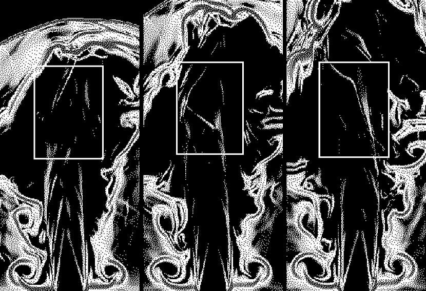
Figure 1.— Schlieren renders (the gradient on an exponential map) of the laboratory frame mass density for the simulation described in the text. The three panels from left to right span the formation and evolution of an oblique shock within the flow. The region extracted for study of magnetic field evolution is shown by the superposed rectangles.

This figure is a low resolution placeholder for astro-ph. The original may be found at http://www.astro.lsa.umich.edu/users/hughes/icon_dir/relproj.html#MAG

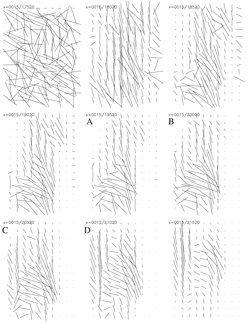
Figure 2.— From left to right and top to bottom, the panels show the magnetic field during $9$ epochs of its evolution during advection by a pre-computed velocity field. The orientation of the lines gives the sense of the dominant magnetic field within regions of $3^{3}$ cells on the same midplane as shown in Figure 1. The length of each line indicates the local magnetic field strength. The central panel corresponds to the central panel of Figure 1. The panels labeled ‘A’, ‘B’, etc. correspond to the panels of Figure 3.

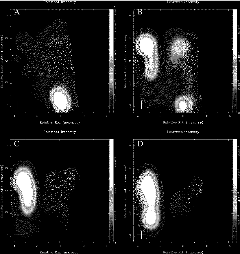
Figure 3.— From upper-left to lower-right, ‘fake’ maps of polarized intensity, computed by performing radiative transfer calculations through the full computational volume for which the $5$th through $8$th epochs shown in Figure 2 (labeled ‘A’, ‘B’, etc.) are slices. Features on these maps may be related to features seen in Figure 2, for example, the ridge of emission in the lower-right panel corresponds to the sheared region of longitudinal field seen to the left of the flow in the last panel of Figure 2. Major differences between the two figures arise because the radiative transfer is probing flow not revealed by the simple cut of Figure 2.

This figure is a low resolution placeholder for astro-ph. The original may be found at http://www.astro.lsa.umich.edu/users/hughes/icon_dir/relproj.html#MAG

References

- Aller et al. (2002) Aller, H. D., Aller, M. F., & Hughes, P. A. 2002, Proceedings of the 6th European VLBI Network Symposium, ed. E. Ros, R. W. Porcas, & J. A. Zensus, (Bonn, Germany: MPIFR), 111
- Aller at al. (1999) Aller, H. D., Hughes, P. A., Freedman, I., & Aller, M. F. 1999, BL Lac Phenomenon, ed. L. O. Takalo, & A. Sillanpää (ASP Conference Series 159), 45
- Attridge et al. (1999) Attridge, J. M., Roberts, D. H., & Wardle, J. F. C. 1999, ApJ, 518, L87
- Beckert & Falcke (2002) Beckert, T., & Falcke, H. 2002, A&A, 388, 1106
- Belloni et al. (2000) Belloni, T., et al. 2000, A&A, 355, 271
- Dar (1998) Dar, A. 1998, ApJ, 500, L93
- Denn et al. (2000) Denn, G. R., Mutel, R. L., & Marscher, A. P. 2000, ApJS, 129, 61
- Duncan & Hughes (1994) Duncan, G. C., & Hughes, P. A. 1994, ApJ, 436, L119
- Fender et al. (2004) Fender, R., et al. 2004, Nature, 427, 422
- Gómez et al. (1993) Gómez, J. L., Alberdi, A., & Marcaide, J. M. 1993, A&A, 274, 55
- Gómez et al. (1994) Gómez, J. L., Alberdi, A., & Marcaide, J. M. 1994, A&A, 284, 51
- Gómez et al. (1994) Gomez, J.-L., Alberdi, A., Marcaide, J. M., Marscher, A. P., & Travis, J. P. 1994, A&A, 292, 33
- Homan & Wardle (2004) Homan, D. C., & Wardle, J. F. C. 2004, ApJ, 602, L13
- Hughes et al. (1989a) Hughes, P. A., Aller, H. D., & Aller, M. F. 1989a, ApJ, 341, 54
- Hughes et al. (1989b) Hughes, P. A., Aller, H. D., & Aller, M. F. 1989b, ApJ, 341, 68
- Hughes et al. (1991) Hughes, P. A., Aller, H. D., & Aller, M. F. 1991, ApJ, 374, 57
- Hughes et al. (2002) Hughes, P. A., Miller, M. A., & Duncan, G. C. 2002, ApJ, 572, 713
- Jones (1988) Jones, T. W. 1988, ApJ, 332, 678
- Jones & O’Dell (1977) Jones, T. W., & O’Dell, S. L. 1977, ApJ, 214, 522
- Jones et al. (1985) Jones, T. W., et al. 1985, ApJ, 290, 627
- Kataoka & Stawarz (2004) Kataoka, J., & Stawarz, L. 2004, astro-ph/0411042
- Kellermann et al. (2004) Kellermann, K. I., et al. 2004, astro-ph/0403320
- Koide et al. (2000) Koide, S., Meier, D. L., Shibata, K., & Kudoh, T. 2000, ApJ, 536, 668
- Komissarov (1999a) Komissarov, S. S. 1999a, MNRAS, 303, 343
- Komissarov (1999b) Komissarov, S. S. 1999b, MNRAS, 308, 1069
- Lister (2003) Lister, M. L. 2003, astro-ph/0309413
- Lyutikov et al. (2004) Lyutikov, M., Pariev, V. I., & Gabuzda, D. C. 2004, astro-ph/0406144
- Mioduszewski et al. (1997) Mioduszewski, A. J., Hughes, P. A., & Duncan, G. C. 1997, ApJ, 476, 649
- Ojha et al. (2004) Ojha, R., et al. 2004, ApJS, 150, 187
- Rosen et al. (1999) Rosen, A., Hughes, P. A., Hardee, P. E., & Duncan, G. C. 1999, ApJ, 516, 729
- Tregillis et al. (2001) Tregillis, I. L., Jones, T. W., & Ryu, D. 2001, ApJ, 557, 475
- Tribble (1991) Tribble, P. C. 1991, MNRAS, 253, 147
- van Putten (1996) van Putten, M. H. P. M. 1996, ApJ, 467, L57
- Zensus (1997) Zensus, J. A. 1997, ARA&A, 35, 607