A Trend Filtering Algorithm for wide field variability surveys

Abstract

We show that various systematics related to certain instrumental effects and data reduction anomalies in wide field variability surveys can be efficiently corrected by a Trend Filtering Algorithm (TFA) applied to the photometric time series produced by standard data pipelines. Statistical tests, performed on the database of the HATNet project, show that by the application of this filtering method the cumulative detection probability of periodic transits increases by up to 0.4 for variables brighter than 11 mag with a trend of increasing efficiency toward brighter magnitudes. We also show that TFA can be used for the reconstruction of periodic signals by iteratively filtering out systematic distortions.

1 Introduction

In the resolute hunt for transiting hot Jupiters, much effort is focused on very small instruments that are capable of observing large area of the sky and gathering data with a photometric precision better than 0.01 mag. There are many projects targeting this goal (see Horne 2003), using instruments with typical apertures of order 10 cm; it has even been argued that the small telescope projects with $\sim 2$ inch diameter optics are the best for this purpose (Pepper, Gould & Depoy 2003).

The attained photometric precision plays a central role in transit signal detection. However, the large field of view and the semi-professional CCD detectors often employed by these low-budget projects drastically amplify some of the standard problems of CCD photometry. These include narrow PSF, crowded field, differential extinction and refraction (see Bakos et al. 2004, hereafter B04, for a more comprehensive summary). Most of the problems become more severe toward fainter magnitudes, where the objects are more affected by time-dependent merging with brighter stars. Most of these, and other hidden effects not only increase the noise of the light curves, but leave their fingerprint in the data as systematic variations, because they vary in a non-smooth fashion over the field, and standard position-dependent smooth transformations applied at various stages of the data reduction do not eliminate them perfectly.

The efficiency of the detection of periodic signals drops dramatically when the light curves become dominated by noise and systematic variations. For example, the BLS method (Kovács, Zucker & Mazeh 2002, hereafter K02), an application used for searching for transits, is efficient on light curves exhibiting a box-shaped dip, but fails to recover transits superposed on strongly variable light curves. These systematics are also harmful in discovering interesting low-amplitude phenomena, such as $\delta$ Scuti or $\gamma$ Dor stars.

Many of the systematic variations in a given light curve are shared by light curves of other stars in the same data set, due to common effects like colour-dependent extinction, or blending of two or more star images (which could produce similar light curve variations in all of them), etc. A solution to remove or reduce these common systematic variations can therefore be devised using the already reduced data. For each target star, one must identify objects in the field that suffer from the same kind of systematics as the target, and apply some kind of optimum filtering of the target light curve based on the light curves of a set of comparison/template stars.

The algorithm to be presented in this paper can be applied to two types of problems. The first application is to remove trends from trend- and noise-dominated time series, thereby increasing the probability of detecting a weak signal (periodic or non-periodic). Secondly, if there is a periodic signal present, the TFA algorithm can be used in a slightly different way to reconstruct also the shape of that signal.

The structure of the paper is the following. Section 2 gives a more detailed description of the systematics and their possible causes. Section 3 describes the mathematical formulation of the TFA algorithm, and Section 4 presents a number of tests of its ability to remove spurious trends from the data. Section 5 explores the increase in detectability of periodic transit signals (using the BLS algorithm) from data after processing with the TFA. Section 6 then investigates the capability of reconstructing the detailed shape and amplitude of such periodic signals, using a variant of the basic algorithm. The paper closes with a brief highlighting of the most important results. Throughout this paper we rely on the database of the HATNet project (see B04).

2 Light curve systematics and their possible sources

The systematic variations might be intrinsic to the data, or they could be due to uncorrected instrumental effects or changing observing conditions, or they could also originate from imperfect data reduction. First we outline the procedure of common photometry reduction methods along with their smooth transformations that correct for trivial systematic variations. Then we proceed to the characterization of the remaining systematics, and discuss them and their possible causes through the examples of the HAT Network light curves.

The typical procedure of wide field photometry either employs flux extraction with aperture-photometry or Point Spread Function (PSF) fitting (e.g., DAOPHOT; Stetson 1987), or uses image subtraction (ISIS; Alard & Lupton 1998; Alard 2000).

In the first type of approach, the instrumental magnitudes of individual frames are transformed to a common magnitude reference system, in order to eliminate the instrumental or observational changes between the epochs. For narrow field surveys, all stars experience the same fractional flux change, and thus the transformation can be treated as a constant magnitude shift with good approximation.

For wide-field surveys, this transformation takes a more complex form, and for convenience it is assumed to be smooth function of the fitting parameters, e.g., of the co-ordinates. The transformation is established by iterative fitting over a substantial sample of stars and subsequent rejection of outlier values. The underlying assumption in this procedure is that CCD images of typical surveys have a large number of stars, and the overwhelming majority of them are non-variable above the noise-level (see Pojmański 2003). We note in passing that other wide field surveys use similar methods in their basic reduction pipelines.

Ideally, after applying the above determined transformation, the resulting light curves should be free of systematic variations, and constant stars should be dominated only by noise. However, omission of some “hidden” parameters, characteristic of the transformation, might lead to systematic spurious variations in the transformed magnitudes; sources with close values of these parameters will exhibit similar variations. Improper functional form of the transformation, or inclusion of variable stars in the fit might lead to similar systematics. Furthermore, because local effects might dominate the light curves (local in position or other parameters), variations remain even after application of the best large scale (smooth) transformations. Such systematics are known to exist in various massive photometric surveys (see, e.g., Drake & Cook 2004 for the MACHO and Kruszewski & Semeniuk 2003 for the OGLE projects) and even in classical CCD observations (Makidon et al. 2004), but in wide field observations they could be especially severe (Alonso et al. 2003).

To give examples, a time-dependent PSF causes variable merging, where the flux contribution of a star to the flux of another star and its background annulus varies (assuming aperture photometry). The extent of systematics induced will depend on the exact configuration of the neighbourhood of the source. Although image subtraction convolves the profiles of the reference frame before the subtraction so that they have (in principle) the same width as on the frame that is analysed, we found that there remain small amplitude correlations with the periodic variation of original PSF widths. Periodic motion of stars across the imperfectly corrected pixels, hot-pixels or bad columns, or simply the gate-structure of front-illuminated pixels can be another cause for systematic variations. Faint stars that fall in the vertical vicinity of stars that are on the saturation limit might be periodically affected by the saturation of the bright source, e.g., with the $29^{d}$ period of moon-cycle through the increased background, or by the nightly variation of extinction, as the object rises and sets.

Here and throughout the paper we employ the database on the moderately crowded ($b=20^{\circ}$) G175 field observed by HATNet. Similar results were obtained with other fields. Observations for G175 were made during the fall and winter of 2003, spanning a compact interval of 202 d with $\sim 3000$ data points for each variable in $I$-band. Nearly 10000 stars down to $I$=12 were analysed with aperture photometry from the field. We employed a 4th order polynomial function of the x and y coordinates to fit each frame’s magnitude system to that of the reference frame. $V$-band data were also taken on selected nights to have complementary colour information on the sources, but this was not incorporated in the above fits. Field G175 observations started or ended every night whenever the field crossed the 35^∘ horizon, and exposures were taken with 5 min resolution with no interruption by observations of another field. There is obviously a (close to sidereal) daily periodicity in the time-base, which has 4–8 hour long sections, and 16 hour or longer gaps. Although the field contains nearly 10000 photometered stars, we present tests on only the 4293 stars, among the 5000 brightest, whose light curve contains at least 2800 points. These bright, intensively observed and accurately photometered stars are the most interesting ones for shallow transit searches. The faintest stars in this sample have $I\sim 11.0$ mag.

After Discrete Fourier Transformation (DFT) of the light curves in the $[0,6]$d^-1 frequency range with 20000 frequency steps, the derived histogram of primary frequencies shows a distribution with high peaks around $n$ d^-1 frequencies, where $n$ is a small integer. The histogram also shows that the 1 and 2d^-1 peaks have double structures, with slight offsets from the exact integer values (see Fig. 1). The double peak structure is attributed to the cadence of 1 sidereal day of the observations and its alias. Other, higher frequency peaks do not show double structure, only an offset, because they are further off from their alias counterparts leaking from the negative frequency regime. A very large fraction (83%) of the peak frequencies fall in the $n\pm 0.02$ d^-1 interval, with $n=$0,1,2,3,4,5. Even excluding the n=0 peak to avoid counting long-periodic variables as the stars showing real systematics, the occurrence rate of integer peak frequencies is still 69%. Weighting the histogram according to the signal-to-noise ratio of the frequency peaks does not significantly alter its appearance.

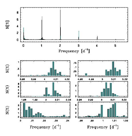
Figure 1: Distribution of the peak frequencies obtained from the DFT of a sample of stars of field G175 (see text for details on the data selection). Largest panel: distribution function in the full bandwidth of the analysis. The sum of the bin occupation number $\rm N$% over the full frequency range is equal to 100. Small panels: blow-ups of the neighbourhood of the peaks. Each bin has a width of $0.002$d^-1 in all panels.

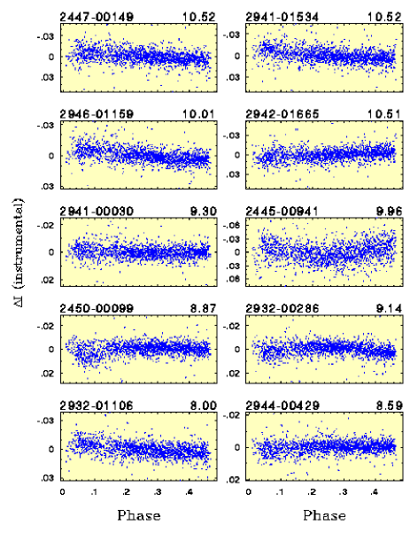
Figure 2: Examples of daily trends in field G175. The numbers on the top of each panel show the star’s identification (GSC number) and the mean value of the instrumental magitude. Plotted are the deviations from this mean value. Phases are computed with $1$ d period and arbitrary epochs.

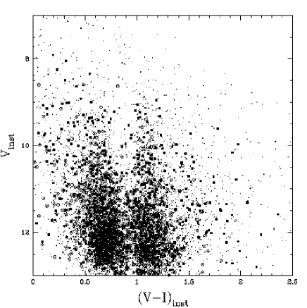
Figure 3: Colour-magnitude diagram of field G175 in instrumental V$-$I vs. V system (small dots) with stars exhibiting strong 1d^-1 (filled boxes) or 2d^-1 (open circles) systematics overplotted.

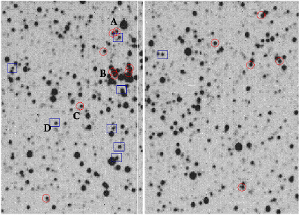
Figure 4: Image section from field G175 with dominant systematic stars marked by circles (1d^-1) and boxes (2d^-1). North is up, East is left, image size is approx. 68′by 49′. White vertical lines are due to bad CCD columns. Most of the 1d^-1 stars are merging with neighbours. The bright star marked as ”A” is on the saturation limit, and might induce the systematic variations seen in the stars South from it. The open cluster NGC2281 (marked as ”B”) is moderately crowded with our 14″pixel-scale, and the merging contributes to the 1d^-1 or 2d^-1 systematics for some of its stars. Nevertheless, there are unexplained cases where isolated stars also show systematic variations, such as ”C” or ”D”.

The systematic variations are of small amplitude, typically $\sim 0.01$ mag. To have a better measure on this quantity, we derived folded and phase-binned light curves (with 100 bins), rejected the lowest and highest 5 points of the phased curve, and determined the amplitude. For instance, the median value of the amplitudes of the 1d^-1 stars is $0.015$ mag, with 85% of them falling below $0.03$ mag. For illustration, in Fig. 2 we exhibit examples of daily trends for a few selected stars in our field.

We searched the observational parameters of HAT for commensurate periodicities the effect of which might get superposed on the data and cause the above mentioned systematics. The trivial daily hour-angle or zenith-distance variation, and the fact that we employ a simple 4th order polynomial transformation that neglects colour dependence suggested that colour-dependent differential extinction should also cause a daily periodicity: redder or bluer than average stars should deviate from others as the field rises or sets. Probably because our data are dominated by other systematics, we found no sign of this when plotting the distribution of higher amplitude $n$ d^-1 stars on a $V-I$ vs. $V$ colour-magnitude diagram (see Fig. 3). However, we noticed that the PSF also varies with close to 1d^-1, which should result in variable merging. Indeed, as shown in Fig. 4, the most prominent systematic variations are exhibited by stars that have close-by merging or almost saturated companions. On the other hand, there remain a few perplexing stars that seem equally merging, but show no strong $n$ d^-1 variations. Early image subtraction results on another field show slightly smaller occurrence of integer cycle-per-day systematics as compared to aperture photometry, which suggest that merging indeed plays a central role. Using more accurate crowded-field photometry, which takes into account the variable stellar profiles, the extent of systematics is somewhat suppressed. There is also sign for slight increase of the occurrence of systematics in the proximity of bad columns. In conclusion, the degree and the appearance of the systematics depend on many factors (position, colour, brightness, merging), among which merging is probably the most important in our case, but not the only one.

3 Trend Filtering Algorithm (TFA)

In this section we give a description of the algorithm in two steps. The first subsection outlines the method and highlights basic problems to be dealt with, whereas the second one reveals more technical details.

3.1 Preliminaries

First of all, it is important to mention that the simplest and seemingly the most general approach to trend filtering would be the application of high-pass filtering on each daily track of observation. In this case with a low-order polynomial or spline fitting we would filter out any variation occurring on a daily time base, presuming that the order of the polynomial (or that of the spline) is properly set. Although we experimented with this approach at the beginning of our tests, we did not find it satisfactory for several reasons: (i) although the daily trends may be the strongest ones, other time scales play a role too; (ii) it is unclear what parts of the variation come from the trend and from the true change in the object; (iii) short tracks of observations may not be treated well in this way at all, because of the increasing chance of mixing intrinsic and systematic variations.

The idea of TFA is based on the observation that in a large photometric database there are many stars with similar systematic effects (this is why they are called ‘systematics’). As we discussed in the previous section, various systematics may be present in the individual objects. We assume that the sample size is large enough for allowing us to select a representative set for all the possible systematics. Once this subsample (template set) is selected, one may try to build up a filter function from these light curves and subtract systematics from the other, non-template light curves.

The first question is how to choose the template set. Because of the lack of a priori information on the type of systematics influencing our target, selection of the template set follows only some very broad guidelines and constitutes basically a random set, drawn from the available database. More details on the template selection are given in Section 3.2.

The second question that must be addressed is how to choose the filter function. Since we have no a priori knowledge on the functional form of the systematics, we take the simplest form of it, i.e., the linear combination of the template light curves.

The third question is how to choose the weights of the template light curves in the filter function. If we assume that the variation in all light curves is caused only by systematics, a natural choice would be a simple least squares criterion for the residuals (observed minus filter-predicted). Since – as we mentioned in Sec. 2 – most of the stars are non-variable, the criterion of minimum variance seems to be a good one for most of the observed stars.

The fourth question is what distortion the TFA process causes in the signal being sought. It is clear that the signal will suffer from some distortion that can be very severe if the time scale and phase of its variation are close enough to those of some of the template time series.

In view of the above considerations, TFA is designed to tackle two types of problems:

(a)

Increase the detection probability by filtering out trends from the trend- and noise-dominated signals.

(b)

Restore the signal form by filtering out trends iteratively from periodic signals, assuming that the period is known.

If the trends are sufficiently small (as compared to the signal amplitude), TFA processing is not necessary for the signal search (i.e., period analysis, application (a)), but (b) can still be a useful utility if the signal turns out to be periodic.

The fifth question is whether the method generates unwanted signal components by chance inclusion of variables in the template set. In classical variable star observations special care was taken to avoid variables among the comparison stars. This was necessary to do so, because variable star magnitudes were obtained by simply subtracting the directly observed magnitudes of the variable star from those of the comparison stars. In the case of TFA the situation is very different. Here we create a linear combination of all template light curves which fits to the target light curve in the best way. This approach tends to fit features that appear in similar forms and in proper timings both in the target and in one or more of the template light curves. Because of the low likelihood this to happen for non-systematic variations, variables in the template set are not expected to influence the TFA filtering. More specifically, templates, containing pure sinusoidal signals will not generate detectable artificial signals in a target of pure white noise (see Appendix A). Of course, this result, referring to the statistical average of the signal detection parameter, does not exclude rare false signal detections due to statistical fluctuations.

3.2 Mathematical formulation

Let us assume that all time series are sampled in the same moments and contain the same number of data points $N$. Let our filter be assembled from a subset of $M$ time series (this is the template set, the method of selection will be discussed later). The filter {$F(i);i=1,2,...,N$} is built up from the following linear combination of the template time series {$X_{j}(i);i=1,2,...,N;j=1,2,...,M$}

$$F(i) = \sum_{j=1}^{M}c_{j}X_{j}(i)\hskip 5.69054pt.$$ (1)

It is assumed that the template time series are zero-averaged (i.e., $\sum_{i=1}^{N}X_{j}(i)=0$ for all $j$). The coefficients {$c_{j}$} are determined through the minimization of the following expression:

$$\cal D = \sum_{i=1}^{N}[Y(i)-A(i)-F(i)]^{2}\hskip 5.69054pt.$$ (2)

Here {$Y(i);i=1,2,...,N$} stands for the target time series being filtered, and {$A(i);i=1,2,...,N$} denotes the current best estimate of the detrended light curve, defined in the following way.

In application (a) (frequency analysis), we start from the assumption that the time series is dominated by systematics and noise, and have no a priori knowledge of any real (periodic or aperiodic) signal in the light curve. Consequently, in this case we set {$A(i)$} equal to the average of the target time series, i.e., $A(i)=\langle Y\rangle\equiv N^{-1}\sum_{k=1}^{N}Y(k)=const$. As we will see in the following sections, this simple choice of {$A(i)$} works very well, except for the rare case when the signal is similar to some of the templates (this happens usually for signals with long periods – comparable to the length of the total time span).

In application (b) (signal reconstruction), we have already established (from previous analysis of the data) that the time series contains a periodic signal. The phase-folded time series can thus be used iteratively to estimate {$A(i)$}. First, an initial filter is constructed using $A(i)=\langle Y\rangle$ as above. The filtered time series {$\hat{Y}(i)\equiv Y(i)-F(i)$} is then phase-folded and binned, then re-mapped to the original time based to give a new estimate of {$A(i)$}, which is in turn fed into equation (2) to compute a new set of filter coefficients {$c_{j}$}. The new filter leads to a better determination of {$A(i)$}, and the iteration continues until some convergence criterion is satisfied. Further details and examples of signal reconstruction are given in Section 6.

Note that the unbiased estimate of the variance of noise of the filtered data can be obtained from the following equation

$$\hat{\sigma}^{2} = {\cal D}/(N-M)\hskip 5.69054pt.$$ (3)

At a more technical level, the main steps of TFA are the following.

(1)

Select $M$ template time series in the full field, distributed nearly uniformly in the field (presumably ensuring uniform sampling also in other parameters, e.g., in colour). Since we have no a priori knowledge on which stars are bona fide variables, the above selection is almost random, except that stars with low number of data points, low brightness and high standard deviation are not selected. Although the result is not sensitive to the actual values of the above limits, it is still better to employ them, in order to avoid any (however small) chance of biasing the target light curve. Nevertheless, for long-periodic target variables there is a higher chance of finding a template member varying on a similar time scale with similar phase. Once the template set is selected, it is fixed throughout the analysis.

(2)

Define the time base to be used by the filter and target time series. Since in modern automated surveys nearly all photometered stars have the same number of data points distributed in the same moments of time, selection of the uniform time base is made on a subsample of the template light curves (containing $\sim 50$ stars in our case). We select the time base from the template light curve that contains the largest number of data points. Occasionally, data points, at some moments defined by the template time base, might be missing in the observed light curve. In these cases they are filled in with the average value of that light curve.

(3)

Compute zero-average template time series by using some criterion for outlier selection (in our case a 5$\sigma$ clipping).

(4)

Compute normal matrix from the above template time series:

$$g_{j,k}=\sum_{i=1}^{N}X_{j}(i)X_{k}(i)\hskip 2.84526pt;\hskip 14.22636ptj,k=1,2,...,M\hskip 5.69054pt,$$ (4)

and compute the inverse of it: {$G_{j,k}$}.

(5)

For each light curve, compute scalar products of the target and template time series:

$$h_{j}=\sum_{i=1}^{N}\tilde{Y}(i)X_{j}(i)\hskip 5.69054pt.$$ (5)

Here the modified target time series {$\tilde{Y}(i)\equiv Y(i)-A(i)$} is also assumed to be free of outliers.

(6)

Compute solution for {$c_{j}$} and apply correction accordingly:

$$c_{j}=\sum_{k=1}^{M}G_{j,k}h_{k}\hskip 5.69054pt,$$ (6)

The corrected time series is computed from

$$\hat{Y}(i)=Y(i)-\sum_{k=1}^{M}c_{j}X_{j}(i)\hskip 5.69054pt,$$ (7)

It is important to make the following comments concerning additional details of the computational implementation.

A significant advantage of the above algorithm is that there is no need to compute the normal matrix for each target separately. This means only the computation of simple array-array and matrix–array products (steps 5–6 above). For period search this is done only once for each star, but for signal reconstruction this is repeated several times (which is still not too time-consuming).

Since the template set is fixed, in principle the normal matrix need only be computed once. In practice, if the target accidentally coincides with one of the template components, the latter must be eliminated from the normal matrix before computing the filter. This requires a reshuffling and inverting of the normal matrix, but it should happen fairly rarely, because of the relative low number of template time series ($\sim 10^{2}\--10^{3}$) compared to the size of database ($\sim 10^{4}$ stars). The CPU request for the initial setup of a filter with few hundred templates is only a few times slower than a single run of the BLS algorithm for transit search. Nevertheless, for large template numbers the extra matrix manipulations increase the execution time substantially. For example, on a 3GHz commercial PC a full BLS analysis of a set of 13000 time series with 2300 data points per time series, 30000 frequency steps per time series and 920 TFA templates required 100 CPU hours. The cost of the non-TFA analysis of the same dataset was only one fifth of it.

The computer memory required by TFA can be quite large. This is mostly because of the template set, since it requires the usage of $N\times M$ floating point array elements. Inversion of the normal matrix may pose also some numerical problems if $M$ is too large, although we have not encountered such problems even for very large $M$ such as $800$. This stability is probably due to the basically uncorrelated noise of the the light curves.

We note that a possible way to decrease the number of templates is to perform a Singular Value Decomposition (SVD, see Press et al. 1992) and employ only the ‘significant’ eigenvectors derived from this decomposition. Although we experimented with SVD at some point, we decided that a clearcut division of the eigenvectors into ‘significant’ and ‘non-significant’ ones was not possible. Therefore, the original ‘brute force’, full template set approach was followed.

There is also the question if magnitude or intensity (flux) values should be used in the above procedure. We experimented with both quantities and finally settled at the direct magnitude values, since no definite advantage was observed to result from a conversion to fluxes.

4 Trend suppression tests

The simplest way to check the most straightforward effect of TFA is to compare the standard deviations of the original and TFA-processed time series. This comparison, of course, will not tell us if all temporal distortions due to trends have been successfully filtered out or not. Nevertheless, it will at least give us some indication on the efficiency of the method.

The effect of decreasing the standard deviation is displayed in Fig. 5. Unbiased estimates of the standard deviations $\sigma$ for the TFA runs were computed with the aid of equation (3) by using a template number of $M=361$. (Originally we set $M=400$, but limitations on the template time series – see Section 3.2 – lowered this value. A similar statement is applied to other template numbers used in this paper.) We see that with the increase of the standard deviation $\sigma$(non-TFA) of the original time series, TFA is likely to introduce significant corrections. This, as expected, means that toward larger $\sigma$(non-TFA) (i.e., at fainter magnitudes) there are time series that are more affected by systematic errors than most of the brighter stars. There are relatively sharp upper and lower boundaries in the decrease of the standard deviation. The existence of the upper boundary at small corrections suggests that all stars are affected by some (however small) systematic errors and TFA is capable of filtering out a substantial part of them. Although TFA also has some side-effects on any real signal in the time series, it suppresses the systematics much more effectively than the signal, as shown by the fact that it leads to a significant increase in detection probability (see Section 5).

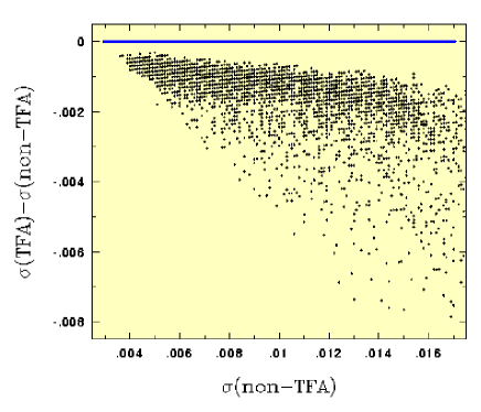
Figure 5: Decrease of the unbiased estimate of the standard deviation of the time series due to the application of TFA. The brightest 4293 stars with greater than 2800 data points per star of field G175 are used. The TFA result was obtained with 361 templates. For better visibility of the minimum decrease in $\sigma$, we plotted a horizontal line to indicate the zero correction level.

In order to examine the question whether the decrease of the standard deviation has also led to the diminishing of the temporal signatures of the systematics, we frequency analysed the original and TFA-processed light curves. The BLS routine was run on both datasets. The analysis was performed in the [0.01,0.99]d^-1 band that covers the period of interest in transit search, but excludes very long periods close to the total time span. We recall that the BLS routine generates several aliases (subharmonics) from the daily trends at frequencies of small integer ratios (see K02). This effect results in the appearance of several aliases in the frequency band chosen for this test. Therefore, the success of TFA in filtering out systematic periodicities can be judged from the above analysis.

The distribution function of the frequencies of the highest peaks obtained on the original, unfiltered dataset is shown in the upper panel of Fig. 6. The large number of stars affected by the daily trends (that appears here mostly at $\sim 0.5$d^-1) is somewhat surprising. Actually, it turns out that 24% of the highest peaks fall in the [0.49,0.51]d^-1 frequency range and about 22% of them appear in the $\pm 0.01$d^-1 neighbourhood of 0.02, 0.33 and 0.66d^-1. It is clear that a simple direct use of the data for transit search would leave a quite substantial part of the sample not utilized because of the domination of trends.

Next, the above analysis is repeated by applying TFA. The result is displayed in the lower panel of Fig. 6. We see that severe aliases due to the daily trends disappeared. Now, as it can be expected for a sample with time series of mostly pure noise, all frequency bins are nearly uniformly occupied. The remaining fluctuations are all of statistical origin, due to the low number of events falling in the narrow bins.

We note in passing that we performed the above test also on the peak frequencies based on DFT spectra. Although at low or moderate template numbers we still got some remnants under the 1% level in the frequency distribution around integer frequencies, at high number of templates we got basically a flat distribution at the 0.3% level, very similar to the one we got for the BLS spectra. We recall that 69% of the DFT peak frequencies obtained by the non-TFA DFT analysis fell in the $\pm 0.02$ d^-1 neighbourhood of positive integer frequencies.

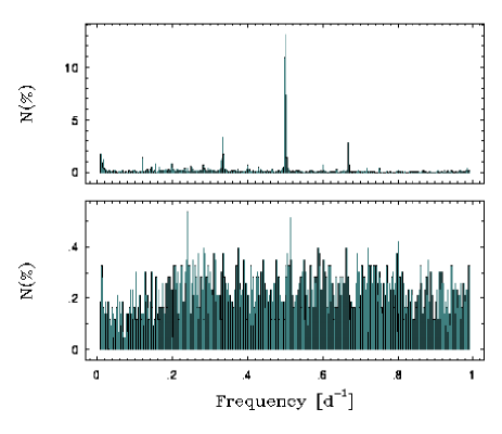
Figure 6: Comparison of the distribution functions of the peak frequencies obtained in the BLS analysis with and without TFA processing (lower and upper panels, respectively). Each bin has a width of $0.002$d^-1. The sum of the bin occupation number $\rm N$% over the full frequency range is equal to 100. The same number of data points and templates are used as in Fig. 5.

5 Transit detection tests

We examine the periodic transit detection capabilities of the BLS method on the TFA-processed light curves. This is done with the aid of various test signals generated from the observed time series and synthetic signals. To each of the 4293 observed, zero-averaged light curve we add the transit signals given in Table 1. Although most of the tests presented in this paper refer to signal #1, the other test signals were also utilized in order to check the efficiency of the method for various signal parameters. Most of these parameters correspond to realistic transit configurations, except perhaps for #5, where the relative duration of the transit is somewhat too long.

In order to illustrate the signal detection capability after applying TFA, in Fig. 7 we exhibit two specifically chosen examples for the extreme improvement one can get for trend-dominated signals. It is obvious that TFA is capable of suppressing a considerable part of the trend without a simultaneous suppression of the periodic signal component. Although the signal also suffers from some amount of suppression, in a very large number of cases this is smaller than the one exerted on the trends. This, as we will see below, ultimately leads to significantly higher detection rates for TFA-processed signals.

Table 1: Parameters of the synthetic signals

No.	$P$[d]	$\delta$[mag]	$\varphi$	$q$
#1	$5.12345$	$-0.015$	$0.73$	$0.03$
#2	$1.23456$	$-0.015$	$0.33$	$0.03$
#3	$1.23456$	$-0.005$	$0.33$	$0.03$
#4	$1.49000$	$-0.015$	$0.33$	$0.03$
#5	$12.5000$	$-0.015$	$0.33$	$0.03$

Comments:

$P$

= Period;

$\delta$

= Depth of the transit;

$\varphi$

= Phase of the transit, defined as $(t_{in}-t(1))/P$, where $t_{in}$ is the moment of the first ingress after $t(1)$, the time of the first item of the time series;

$q$

= Relative length of the transit, defined as the ratio of the actual transit length and the period.

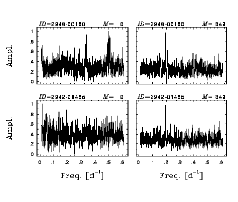
Figure 7: Examples of the signal detection capability of TFA. In both cases test signal #1 was added to the observed light curves of the stars given by the identification numbers in the headers.Left column: BLS spectra of the non-TFA (original) test light curves. Right column: BLS spectra of the TFA test light curves. Template numbers are shown in the headers. The spectra are normalized to unity in each panel separately.

In order to compare the detection rates obtained from the original and TFA-processed light curves, we need to define the meaning of the word ‘detection’. Based on the frequency spectrum, we employ the following two criteria to regard a peak frequency as being identical with the injected test frequency.

$-$

The highest peak in the BLS spectrum should have a frequency in the $[f_{\rm test}-0.001,f_{\rm test}+0.001]$d^-1 interval, where $f_{\rm test}$ is the frequency of the test signal, in the present case of signal #1 it is equal to 0.1952d^-1.

$-$

The Signal to Noise Ratio (SNR) of the highest peak in the frequency spectrum must be greater than 6. The definition of SNR is the following: ${\rm SNR}=[p({\rm highest\hskip 5.69054ptpeak})-\langle p\rangle]/\sigma(p)$. Here $p$ denotes the BLS statistics (denoted by SR in K02), $\langle p\rangle$ is the average power in the frequency band analysed, $\sigma(p)$ is the standard deviation of the spectrum (we omit large peaks in the computation of $\langle p\rangle$ and $\sigma(p)$).

The above lower limit of SNR is somewhat arbitrary and it is a compromise between avoiding too high false alarm rates but not losing too many positive peak identifications. At the end of this section we will discuss the effect of posing a more stringent condition on SNR.

For the characterization of the detection probability, we introduce the Cumulative Detection Probability (CDP) that is defined in the following way:

$${\rm CDP} = {N_{d}(m<I)\over N_{nv}(m<I)}\hskip 5.69054pt.$$ (8)

Here $N_{d}(m<I)$ denotes the number of detections for test signals brighter than $I$ magnitudes, $N_{nv}(m<I)$ stands for the number of non-variable stars in this magnitude range. Because some 5–10% of the stars in the sample are true variables and they will either dominate the signal or decrease the SNR of the test signal below the detection limit, conservatively we take $N_{nv}(m<I)=0.95N_{t}(m<I)$, where $N_{t}(m<I)$ is the total number of stars brighter than $I$ magnitude. Because in this test all stars have injected transit signals, the detection rates to be derived have nothing to do with the true incidence rates of transits in our sample or in stars in general. The sole purpose of this test is to find out by how much do we increase the chance of detection by applying TFA.

The derived CDPs on the sample of 4293 stars are shown in Fig. 8. The somewhat jagged variation of the curves for bright stars is attributed to the relatively small sample size for these stars.

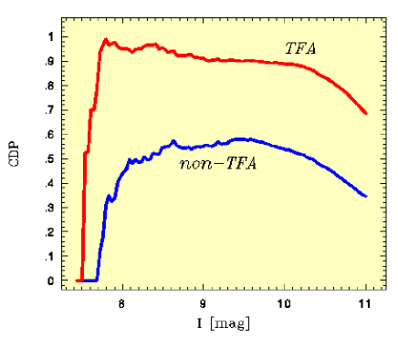
Figure 8: Cumulative Detection Probability for test signal #1 in the presence of observational noise. All cases considered have SNR$>6$. The TFA result was obtained with 595 templates.

It is clear from this figure that TFA introduces a substantial improvement in our detection capability. The high and almost constant detection rate down to $\sim 10.2$ mag indicates the steady performance of TFA. The situation changes at fainter magnitudes, when the random photometric noise becomes higher. This, coupled with the not too favorable combination of period, phase and data distribution for signal #1, results in a definite decrease in CDP at fainter magnitudes. The decrease of the detection probability is more visible if we check narrow magnitude intervals. For example, for test signal #1, the detection probability decreases from $0.45$ to $0.08$ for the raw data when moving from the $\pm 0.1$ range of $10.0$ mag to the same range of $11.0$ mag. The same probabilities for the TFA-processed light curves are $0.87$ and $0.27$, respectively. For short period signals the detection capability (both for the original and TFA-processed time series) is greater than for long period signals as is to be exhibited at the end of this section.

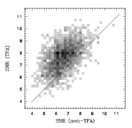
Figure 9: Comparison of the SNRs obtained for test signals #1 with BLS spectra satisfying only the frequency constraint for detectability. Shading is proportional to the number of cases (darker regions contain larger number of cases). The TFA result was obtained with 595 templates.

It is also important to characterize the change in the SNR when we lift the SNR$>6$ constraint. Then, by keeping only the frequency constraint given above, and plotting the SNR values for the variables satisfying this single constraint (both in the TFA-processed and original datasets), we get the plot displayed in Fig. 9. Again, the improvement introduced by TFA is obvious. Many transits, with SNR$<6$ in the original time series become confidently ‘discovered’ after applying TFA. However, it is also seen that there are cases when the original time series have higher SNR. Although this feature is expected to be rare, it is not too surprising. While TFA suppresses mostly those features in the target light curve that can also be found in the template set, it may happen that during this procedure, features (i.e., intrinsic variability) not representative of the trends, become also suppressed. This effect of TFA is not too harmful at higher SNR values (e.g., for SNR$>8$), because the signal will be securely detected in both datasets, albeit with a somewhat smaller significance for the TFA-processed time series. The situation becomes worse at lower SNR, when the signal may become suppressed under the detection limit.

In order to get a more quantitative insight into this phenomenon, we checked the number of cases when the signal was detected in the original, but escaped detection in the TFA-processed time series. By performing this and the opposite check with two different template numbers and detection limits for various test signals, we obtained the results shown in Table 2. It is seen that the number of such exclusive detections is always much higher among the TFA-processed light curves. In addition, the application of higher template numbers increases the number of cases when only TFA is capable to detect the signal. Nevertheless, it seems that there is almost always a relatively small fraction of stars that escape detection in TFA, because of the unwanted side effect of trend suppression.

Table 2: Mutually exclusive detections for various test signals

No.	$N_{6}^{361}$	$N_{6}^{820}$	$N_{8}^{361}$	$N_{8}^{820}$
#1	56	59	29	21
	1414	1696	692	1452
#2	0	1	0	0
	619	704	845	930
#3	24	28	5	8
	1014	1139	838	980
#4	56	82	37	69
	1162	1264	1176	1323
#5	0	19	0	0
	0	1957	0	177

Comments:

$-$

$N_{i}^{j}=$ Number of exclusive detections obtained with SNR$>i$ and template number $j$;

$-$

Upper rows: not detected using TFA-processed data, but detected using raw data

$-$

Lower rows: detected using TFA-processed data, but not detected using raw data

It is interesting to compare the effect of various signal parameters on the detection probability. As before, here we limit ourselves to the test signals given in Table 1. For each test signal we check the CDP obtained at two magnitude and at two SNR levels entering in the detection condition discussed above. Changing the SNR level is illustrative for the expected decrease of CDP when one is aimed at detections with high confidence and with practically zero false alarm rate. The derived CDP values are given in Table 3. As expected, TFA always yields higher CDP, independent of the signal. The gain is of course smaller for cases of high signal-to-noise ratio, such as for signal #2. It is noticeable that single site observations inevitably lead to bias toward discovering short periodic transits (see also Brown 2003). For example, test signals #2 and #5 have the same parameters except for their periods. This results in a dramatic difference in CDP. In terms of the signal-to-noise ratio of the frequency spectra, SNR rarely hits 8 even when TFA is employed for #5, whereas an overwhelming majority of the spectra of the original (non-TFA) data for #2 have SNR$>8$ and quite often above 10 (reaching a maximum value of 25).

Table 3: CDP for various test signals

No.	$CDP_{6}^{10}$	$CDP_{6}^{11}$	$CDP_{8}^{10}$	$CDP_{8}^{11}$
#1	0.54	0.35	0.05	0.03
	0.91	0.73	0.64	0.38
#2	0.90	0.83	0.86	0.76
	1.00	1.00	0.99	0.98
#3	0.36	0.17	0.19	0.08
	0.79	0.44	0.68	0.32
#4	0.72	0.51	0.62	0.37
	0.95	0.79	0.92	0.67
#5	0.05	0.03	0.00	0.00
	0.73	0.50	0.08	0.04

Comments:

$-$

$CDP_{i}^{j}=$ CDP at magnitude $j$ for stars with SNR$>i$;

$-$

Upper rows: non-TFA results, lower rows: TFA results with 820 templates.

6 Signal reconstruction

In Section 3 we emphasized that when using TFA for signal detection, we assume that the signal is trend- and noise-dominated, therefore the use of constant detrended signal {$A(i)=$const} seems to be justified. Nevertheless, the original signal will suffer from some level of distortion, because of the requirement of minimum variance for the signal that is assumed to be constant. It is clear that for non-periodic signals of arbitrary shape, sampled unevenly and gapped in time, is very difficult to make any reasonable initial guess on the original signal form. Therefore, the reconstruction method developed in this section can be applied only to periodic time series.

The main step of the algorithm is the iterative approximation of {$A(i)$}. This has already been described in Section 3. It is important to find a good method to estimate {$A(i)$} at each step of iteration. Here we employ the simple method of bin averaging to derive the updated set of {$A(i)$} at each step of iteration. Of course, the reliable estimate of {$A(i)$} requires the use of proper number of bins in order both to allow an ample sampling of the light curve and to ensure statistical stability due to observational noise. Although in our case of $\sim 3000$ data points per light curve even $100$ bins give a reasonable noise averaging, usually lower number of bins (e.g., 50) are also acceptable, because of the smooth shapes of most of the light curves.

Once the signal shape is more accurately determined by the above general method, one may proceed further and utilize this information to derive a more specific model for the signal shape. For example, if the signal turns out to be of box-shaped, one can use the BLS routine to get more accurate approximation for {$A(i)$}. However, it is emphasized that this second level of filtering can be used only if the first, more general method firmly supports our assumption on the signal form. Otherwise the output will be biased through our incorrect assumption on the signal shape.

Iteration on the folded light curve continues until the relative difference between the standard deviations of the residuals (see equations (2) and (3)) in the successive iterations become under a certain limit. We set this limit at $10^{-3}$.

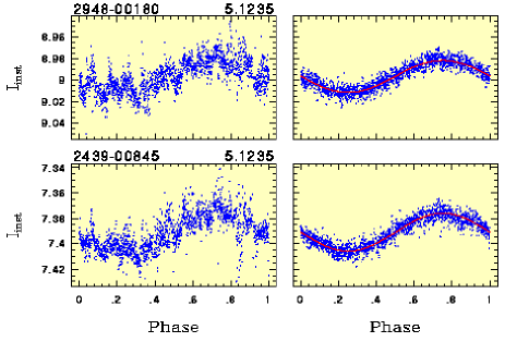
Figure 10: Reconstruction of a sinusoidal test signal with the aid of iterative TFA filtering. Left column: original folded signal. Right column: TFA-filtered signal with the synthetic signal shown by continuous line. Identifiers (GSC numbers) of the stars employed in the generation of the test signals and the corresponding periods are given in the headers of the panels on the left. We used 595 template light curves and bin averaging in the TFA filtering.

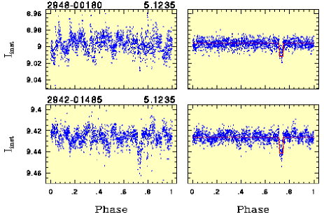
Figure 11: Reconstruction of our standard box-shaped test signal #1 (see Table 1) with the aid of iterative TFA filtering. Notation, method of reconstruction and the TFA parameters used are the same as in Fig. 10.

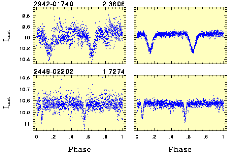
Figure 12: Examples of the reconstruction of the light curves of observed intrinsic variables with the aid of iterative TFA filtering. Notation, method of reconstruction and the TFA parameters used are the same as in Fig. 10.

For the illustration of the efficiency of the method, first we generate a sinusoidal test signal in the same way we did in the case of the transit signals in Section 5 (i.e., by injecting the synthetic signal in the real light curves). The period of the injected signal is the same as that of test signal #1 (see Table 1), whereas its amplitude is $0.015$ mag. We use 100 bins for the estimation of the detrended light curve {$A(i)$} during each step of iteration. In Fig. 10 we show two examples of the substantial improvement obtained after TFA filtering. As we see, the TFA-filtering returned the original signal form without suppressing the amplitude or modifying the phase.

The second example in Fig. 11 shows the result for our standard box-shaped transit signal (#1, see Table 1). Again, it is seen that the signal can be completely scrambled by systematics, yet TFA is able to reconstruct the original signal shape (and also to find the correct period).

In order to quantify the accuracy of the estimated parameters when TFA signal reconstruction is used, we compare the derived transit parameters with those obtained in the course of the BLS period search (i.e., without iterative TFA correction of the transit shape). In Table 4 we show the averages and standard deviations of the three parameters (computed only from the significant detections, as defined in Section 5). We see that both the phase and the width are estimated with the same accuracy in both cases, with no apparent systematic errors. However, the depth is substantially underestimated if TFA is applied without iterative signal reconstruction.

Table 4: Estimated parameters of test signal #1

Parameter	Average	$\sigma$
$\delta$	$-0.0111$	0.0013
	$-0.0147$	0.0016
q	0.0290	0.0019
	0.0290	0.0019
$\varphi$	0.7307	0.0043
	0.7308	0.0043

Comments:

$-$

Transit parameters are described in Table 1.

$-$

Only significant detections (as defined in Section 5) have been considered.

$-$

At each parameter the upper row refers to the values obtained without, whereas the lower one with iterative TFA filtering.

$-$

$\sigma$ denotes the standard deviations of the detected signal parameters.

Finally, in Fig. 12 we show two real examples for signal reconstruction from the G175 database. As in all of our examples presented in this section, we used bin averaging applicable for arbitrary-shaped signals. Although these examples are not representative of the overall effect of TFA on the other variables in the database, they clearly show the size of improvement one may get in cases heavily corrupted by systematics.

7 Conclusions

Current studies indicate that the incidence rate of hot Jupiters is much lower than it was believed a few years ago (Brown 2003). Although we do not have good observational constraint yet for bright Galactic field stars, based on the OGLE survey of faint Galactic Bulge stars and the very low number of positive cases obtained by spectroscopic follow-ups (Alonso et al. 2004; Pont et al. 2004, and references therein), the predicted low incidence rate could be close to reality. Therefore, it is of prime importance to develop effective methods both for data reduction and for subsequent data analysis. The goal to be reached by photometric surveys targeting extrasolar planets is twofold: (i) to reach photometric accuracy close to the photon noise; (ii) to minimize systematic effects leading to coloured noise and therefore seriously jeopardizing the discovery rate. Although current sophisticated data reduction techniques (e.g., Differential Image Analysis by Alard & Lupton 1998; Alard 2000) may help to reach the near photon noise limit and minimize systematic effects, the latter seems to be never eliminated completely. Systematic effects, usually appearing on a daily timebase, are present even in observations that cover small area of the sky per frame (MACHO, OGLE). Wide field surveys have severe additional disadvantages (e.g., narrow PSF, strong nonlinearities in the magnitude/position transformations, etc.) that amplify further the systematic effects and thereby make subsequent data analysis more difficult.

Since the appearance of systematics seems to be generic, it is important to devise a method that is capable of filtering out systematics from the time series photometry in a post-reduction phase. The reason why such an approach may work is that in standard data reduction pipelines the photometry is done through image processing of snapshots. Therefore, these types of data reduction methods are unable to consider the time series properties of the database. The Trend Filtering Algorithm (TFA) described in this paper takes into consideration the temporal behavior of the data by constructing a linear filter from a template set of time series chosen from the database to be analysed. Our TFA is capable to handle two problems:

(a)

Create optimally filtered time series for frequency analysis;

(b)

Reconstruct periodic signals scrambled by systematics.

In both cases the optimization of the filter is made in the standard least squares sense. In application (a) the signal is assumed to be trend- and noise-dominated, whereas in (b) this assumption is not made and the filtered signal is iteratively built up by applying case (a) assumption on the residual (observed minus cycle-averaged) time series.

Tests made on the database of the HATNet project have shown that by the application of TFA the signal detection rate (the Cumulative Detection Probability – CDP) increases by up to 0.4 for stars brighter than 11 mag. The improvement in the Signal to Noise Ratio (SNR) is often spectacular, leading to secure discoveries from signals originally completely hidden in the systematics. Once the period is found, the signal can be reconstructed by applying TFA iteratively as mentioned above.

Results presented in this paper indicate that there is a steady increase in CDP and SNR even for template numbers above 500. This suggests that systematics show up in many different forms and one needs to consider as many of them as possible when targeting the detection of weak signal components. Limitations to very high template numbers are set only by the size of the sample, the number of the data points, statistical and numerical stability and computational power.

Appendix A

The purpose of this Appendix is to show that templates containing periodic signals do not induce similar components at the level of detection in a pure noise target time series. For simplicity we discuss only the case for a single template. The result holds also for arbitrary number of orthogonal templates.

Let the target {$y_{i};i=1,2,...,n$} be equal to a pure Gaussian white noise series {$\eta_{i}$} with the following properties

$$E(\eta_{i})=0\hskip 14.22636ptE(\eta_{i}\eta_{j})=\delta_{ij}\sigma^{2}\hskip 5.69054pt,$$ (9)

where $E(.)$ denotes the expectation value, $\delta_{ij}$ is the Kronecker delta function, $\sigma$ is the standard deviation. The template is a simple harmonic function in the form of

$$x_{i}=A\sin\Phi_{i}\hskip 5.69054pt,$$ (10)

where $\Phi_{i}=\omega_{0}t_{i}+\varphi_{0}$. The TFA minimization criterion leads to the following expression for the estimate of the filtered target {$\hat{y}_{i}$}

$$\hat{y}_{i}=\eta_{i}-a\sin\Phi_{i}\hskip 5.69054pt;\hskip 5.69054pta={2\over n}\sum_{j=1}^{n}\eta_{j}\sin\Phi_{j}\hskip 5.69054pt.$$ (11)

It is seen that the amplitude of the induced periodic signal is expected to be very small, because it is computed through the Fourier transformation of the noise.

In order to compute the power spectrum of {$\hat{y}_{i}$} at arbitrary test frequency $\omega$, we take the Fourier transform of {$\hat{y}_{i}$}. For the sine and cosine transforms we get

$$S={2\over n}\sum_{i=1}^{n}\eta_{i}g_{i}\hskip 5.69054pt;\hskip 5.69054ptC={2\over n}\sum_{i=1}^{n}\eta_{i}f_{i}\hskip 5.69054pt,$$ (12)

where

$$f_{i}=\cos\omega t_{i}-\alpha\sin\Phi_{i}\hskip 5.69054pt;\hskip 5.69054pt\alpha={2\over n}\sum_{j=1}^{n}\sin\Phi_{j}\cos\omega t_{j}$$

$$g_{i}=\sin\omega t_{i}-\beta\sin\Phi_{i}\hskip 5.69054pt;\hskip 5.69054pt\beta={2\over n}\sum_{j=1}^{n}\sin\Phi_{j}\sin\omega t_{j}\hskip 5.69054pt.$$ (13)

By using the properties of equation (A1), we get for the expectation value of the power $P(\omega)=S^{2}+C^{2}$

$$E(P(\omega))={4\sigma^{2}\over n^{2}}\Bigl{[}n-(\alpha^{2}+\beta^{2})(n-\sum_{i=1}^{n}\sin^{2}\Phi_{i})\Bigr{]}\hskip 5.69054pt.$$ (14)

By omitting sums of oscillating terms, far from the template frequency $\omega_{0}$ we get the well-known result for the average noise power (see, e.g., Kovács 1980)

$$E(P(\omega))={4\sigma^{2}\over n}\hskip 5.69054pt.$$ (15)

At the template frequency, with the above assumption on the oscillating terms, we have $\alpha^{2}+\beta^{2}\approx 1$ and $\sum_{i=1}^{n}\sin^{2}\Phi_{i}\approx n/2$. Therefore, we get

$$E(P(\omega_{0}))={2\sigma^{2}\over n}\hskip 5.69054pt.$$ (16)

Thus, $E(P(\omega_{0}))/E(P(\omega))=1/2$, which means that TFA (on the average) does not induce extra signal component in the filtered time series; on the contrary, it ‘whitens out’ (in the statistical sense) even the pure noise target, resulting in a decrease of a factor of two in the average power at the template frequency.

References

- [1] Alard C., 2000, A&AS, 144, 363
- [2] Alard C., Lupton R. 1998, ApJ, 503, 325
- [3] Alonso R., Belmonte J. A., Deeg H., Brown T. M., 2003, in ‘Scientific Frontiers in Research on Extrasolar Planets’, Eds.: D. Deming, S. Seager, ASP Conf. Ser., 294, 371
- [4] Alonso R., Brown T. M., Torres G. et al., 2004, ApJ (Letters), to be published (astro-ph/0408421)
- [5] Bakos G., Noyes R. W., Kovács G., Stanek K. Z., Sasselov D. D., Domsa I., 2004, PASP, 116, 266 (B04)
- [6] Brown T. M., 2003, Ap. J., 593, 125
- [7] Drake A. J., Cook K. H., 2004, ApJ, 604, 379
- [8] Horne K., 2003, in ‘Scientific Frontiers in Research on Extrasolar Planets’, Eds.: D. Deming, S. Seager, ASP Conf. Ser., 294, 36
- [9] Kovács G., 1980, Ap&SS 69, 485
- [10] Kovács G., Zucker S., Mazeh, T., 2002, A&A, 391, 369 (K02)
- [11] Makidon R. B., Rebull L. M., Storm S. E., Adams M. T., Patten B. M., 2004, AJ, 127, 2228
- [12] Kruszewski A., Semeniuk I., 2003, Acta Astr., 53, 241
- [13] Pepper J., Gould A., Depoy D. L., 2003, Acta Astr., 53, 213
- [14] Pojmański G., 2003, Acta Astr., 53, 341
- [15] Pont F., Bouchy F., Queloz D., Santos N. C., Melo C., Mayor M., Udry S., 2004, A&A (Letters), to be published (astro-ph/0408499)
- [16] Press W. H., Teukolsky S. A., Vetterling W. T., Flannery B. P., 1992, Numerical Recepies in Fortran, The Art of Scientific Computing, Cambridge University Press
- [17] Stetson P. B., 1987, PASP, 99, 191