Spectroscopic Constants, Abundances, and Opacities of the TiH Molecule

Abstract

Using previous measurements and quantum chemical calculations to derive the molecular properties of the TiH molecule, we obtain new values for its ro-vibrational constants, thermochemical data, spectral line lists, line strengths, and absorption opacities. Furthermore, we calculate the abundance of TiH in M and L dwarf atmospheres and conclude that it is much higher than previously thought. We find that the TiH/TiO ratio increases strongly with decreasing metallicity, and at high temperatures can exceed unity. We suggest that, particularly for subdwarf L and M dwarfs, spectral features of TiH near $\sim$0.52 $\mu$m , 0.94 $\mu$m , and in the $H$ band may be more easily measurable than heretofore thought. The recent possible identification in the L subdwarf 2MASS J0532 of the 0.94 $\mu$m feature of TiH is in keeping with this expectation. We speculate that looking for TiH in other dwarfs and subdwarfs will shed light on the distinctive titanium chemistry of the atmospheres of substellar-mass objects and the dimmest stars.

1 INTRODUCTION

The discovery of the new spectroscopic classes L and T (Nakajima et al. 1995; Oppenheimer et al. 1995; Burgasser et al. 2000abc; Kirkpatrick et al. 1999) at lower effective temperatures, (T${}_{\rm eff}\,$), (2200 K$\rightarrow$700 K) than those encountered in M dwarfs has necessitated the calculation (and recalculation) of thermochemical and spectroscopic data for the molecules that predominate in such cool atmospheres. At temperatures ($T$) below 2500 K, a variety of molecules not dominant in traditional stellar atmospheres become important. Though a few molecules, such as TiO, VO, CO, and H₂O, have been features of M dwarf studies for some time, for the study of L and T dwarfs, even for solar metallicities, the molecules CH₄, FeH, CrH, CaH, and MgH take on increasingly important roles. The last four metal hydrides are particularly important in subdwarfs, for which the metallicity is significantly sub-solar. In subdwarf M dwarfs, the spectral signatures of “bimetallic” species such as TiO and VO weaken, while those of the “monometallic” hydrides, such as FeH, CaH, CrH, and MgH, increase in relative strength. This shift from metal oxides to metal hydrides in subdwarfs is an old story for M dwarfs, but recently, Burgasser et al. (2003) and Burgasser, Kirkpatrick & Lépine (2004) have discovered two L dwarf subdwarfs, 2MASS J05325346+8246465 and 2MASS J16262034+3925190, and this shift to hydrides is clear in them as well. In fact, Burgasser, Kirkpatrick & Lépine (2004) have recently tentatively identified titanium hydride (TiH) in 2MASS J0532 at $\sim$0.94 $\mu$m , a molecule that heretofore had not been seen in “stellar” atmospheres (see also Burgasser 2004).

In support of L and T dwarf studies, we have an ongoing project to calculate line lists, line strengths, abundances, and opacities of metal hydrides. Burrows et al. (2002) and Dulick et al. (2003) have already published new calculations for CrH and FeH, respectively. With this paper, and in response to the recent detection of TiH in 2MASS J0532, we add to this list new spectroscopic, thermochemical, and absorption opacity calculations for TiH. In §2, we summarize the spectroscopic measurements we use to help constrain the spectroscopic constants of TiH. We continue in §3 with a discussion of the computational chemistry calculations we performed in conjunction with our analysis of the laboratory work on TiH. In §5, we calculate TiH abundances with the newly-derived thermochemical data and partition functions and find that the TiH abundances, while not high, are much higher than previous estimates. We also describe the updates to our general chemical abundance code that are most relevant to titanium chemistry. Section 6 describes how we use these lists to derive opacities at any temperature and pressure and §7 summarizes our general conclusions concerning these updated TiH ro-vibrational constants, abundances, and opacities.

2 SUMMARY OF SPECTROSCOPIC WORK

Although spectra of TiH have been available for several decades (Smith & Gaydon 1971), major progress on the spectral assignment has been made only recently (Steimle et al., 1991; Launila & Lindgren, 1996; Andersson, Balfour & Lindgren, 2003; Andersson et al., 2003). The spectrum of TiH was first observed by Smith and Gaydon in 1971 in a shock tube and a tentative ${}^{4}\Delta-^{4}\Phi$ assignment was proposed for a band near 530 nm (Smith & Gaydon 1971). By comparing the TiH measurements (Smith & Gaydon 1971) with the spectra of $\alpha$ Ori, $\alpha$ Sco, and $\delta$ Vir, Yerle (1979) proposed that TiH was present in stellar photospheres. Yerle’s tentative TiH assignments in these complex stellar spectra are very dubious.

The first high-resolution investigation of TiH was made by Steimle et al. (1991) who observed the laser excitation spectrum of the 530-nm band. After rotational analysis, this band was assigned as the ${}^{4}\Gamma_{5/2}-X^{4}\Phi_{3/2}$ sub-band of a ${}^{4}\Gamma-X^{4}\Phi$ transition (called the $B^{4}\Gamma-X^{4}\Phi$ transition in the present paper). The spectrum of the 530-nm transition of TiH was later investigated by Launila and Lindgren (1996) by heating titanium metal in an atmosphere of about 250 Torr of hydrogen, and the spectra were recorded using a Fourier transform spectrometer. The assignment of the 530-nm system was confirmed as a ${}^{4}\Gamma-X^{4}\Phi$ transition by the rotational analysis of the four sub-bands of the 0-0 vibrational band. The spectrum of the analogous ${}^{4}\Gamma-X^{4}\Phi$ transition of TiD has recently been studied at high resolution using a Fourier transform spectrometer (Andersson, Balfour & Lindgren, 2003). TiD was also produced by heating titanium powder and 250 Torr of D₂ in a King furnace. The rotational analysis of the ${}^{4}\Gamma_{7/2}-X^{4}\Phi_{5/2}$ and ${}^{4}\Gamma_{5/2}-X^{4}\Phi_{3/2}$ sub-bands produced the first rotational constants for TiD (Andersson, Balfour & Lindgren, 2003).

In a more recent study, the spectra of TiH and TiD were observed in the near infrared (Andersson et al., 2003) using the Fourier transform spectrometer of the National Solar Observatory at the Kitt Peak. The molecules were produced in a titanium hollow cathode lamp by discharging a mixture of Ne and H₂ or D₂ gases. A new transition with complex rotational structure was observed near 938 nm and was assigned as a ${}^{4}\Phi-X^{4}\Phi$ transition (called the $A^{4}\Phi-X^{4}\Phi$ transition in the present paper). The complexity of this transition is due to the presence of perturbations, as well as overlapping from another unassigned transition (Andersson et al., 2003). The spectroscopic constants for the TiH and TiD states were obtained by rotational analysis of the 0-0 band of the four sub-bands.

In other experimental studies of TiH, a dissociation energy of 48.9$\pm$2.1 kcal mole^-1 was obtained by Chen et al. (1991) using guided ion-beam mass spectrometry. The fundamental vibrational intervals of 1385.3 cm^-1 for TiH and 1003.6 cm^-1 for TiD were measured from matrix infrared absorption spectra (Chertihin & Andrews, 1994). The molecules were formed by the reaction of laser-ablated Ti atoms with H₂ or D₂ and were isolated in an argon matrix at 10 K.

There have been several previous theoretical investigations of TiH. Ab initio calculations for TiH and other first-row transition metal hydrides have been carried out by Walch and Bauschlicher (1983), Chong et al. (1986), and Anglada et al. (1990). Spectroscopic properties of the ground states of the first row transition metal hydrides were predicted in these studies. Chong et al. (1986) and Anglada et al. (1990) have also calculated spectroscopic properties of some low-lying states. In a recent study the spectroscopic properties of the ground and some low-lying electronic states of TiH were computed by Koseki et al. (2002) by high level ab initio calculations that included spin-orbit coupling. The potential energy curves of low-lying states were calculated using both effective core potentials and all-electron approaches.

3 COMPUTATIONAL CHEMISTRY METHODS AND RESULTS

To supplement the sparse spectroscopic measurements summarized in §2, we calculate the spectroscopic constants, transition dipole moments, line strengths, and ro-vibrational constants of the TiH molecule using standard ab initio quantum chemical techniques. The orbitals of the TiH molecule are optimized using a state-averaged complete-active-space self-consistent-field (SA-CASSCF) approach (Roos, Taylor & Siegbahn 1980), with symmetry and equivalence restrictions imposed. Our initial choice for the active space include the Ti 3d, 4s, and 4p orbitals and the H 1s orbital. In $C_{2v}$ symmetry, this active space corresponds to four $a_{1}$, two $b_{1}$, two $b_{2}$, and one $a_{2}$ orbital, which is denoted (4221). Test calculations showed that this active space is much too small to study both the $B{}^{4}\Gamma-{}X^{4}\Phi$ and $A{}^{4}\Phi-{}X^{4}\Phi$ systems simultaneously. In fact, no practical choice for the active space was found that allowed the study of both band systems simultaneously. Therefore, the two band systems are studied using separate calculations. For the $B{}^{4}\Gamma-{}X^{4}\Phi$ system, the (4221) active space is sufficient. In this series of calculations, two ${}^{4}\Delta$ states and one state each of ${}^{4}\Pi$, ${}^{4}\Phi$, and ${}^{4}\Gamma$ are included in the SA procedure, with equal weight given to each state. In the $A{}^{4}\Phi-{}X^{4}\Phi$ SA-CASSCF calculations, it was necessary to increase the active space, and our final choice is a (7222) active space that has two additional $\sigma$ orbitals and one additional $\delta$ orbital, relative to the (4221) active space. Only the two ${}^{4}\Phi$ states are included in the SA-CASSCF calculations for the $A{}^{4}\Phi-{}X^{4}\Phi$ system.

More extensive correlation is included using the internally contracted multireference configuration interaction (IC-MRCI) approach (Werner & Knowles, 1988; Knowles & Werner, 1988). All configurations from the CASSCF calculations are used as references in the IC-MRCI calculations. The valence calculations correlate the Ti 3d and 4s electrons and the H electron, while in the core+valence calculations the Ti 3s and 3p electrons are also correlated. The Ti 3s- and 3p-like orbitals are in the inactive space so they are doubly occupied in all reference configurations. The effect of higher excitations is accounted for using the multireference analogue of the Davidson correction (+Q) (Langhoff & Davidson 1974). Since the IC-MRCI calculations are performed in $C_{2v}$ symmetry, the $\Delta$ and $\Gamma$ states are in the same symmetry as are the $\Phi$ and $\Pi$ states. Thus, for the $B{}^{4}\Gamma-{}X^{4}\Phi$ calculation, the IC-MRCI reference space included three roots of ${}^{4}A_{1}$ symmetry and two roots of ${}^{4}B_{1}$ symmetry. For the $A{}^{4}\Phi-{}X^{4}\Phi$ system, the reference space includes four roots of ${}^{4}B_{1}$ symmetry since there are two ${}^{4}\Pi$ states below the $A{}^{4}\Phi$ state.

Scalar relativistic effects are accounted for using the Douglas-Kroll-Hess (DKH) approach (Hess, 1986). For Ti we use the (21s16p9d4f3g1h)/[7s8p6d4f3g1h] quadruple zeta (QZ) 3s3p basis set (Bauschlicher, 1999), while for H we use the correlation-consistent polarized valence QZ set (Dunning, 1989). The nonrelativistic contraction coefficients are replaced with those from DKH calculations. All calculations are performed with Molpro2002 (Werner & Knowles, 2002) that is modified to compute the DKH integrals [C.W. Bauschlicher, unpublished].

The transition dipole moments for the forbidden ${}^{4}\Pi$-${}^{4}\Gamma$ and ${}^{4}\Pi$-${}^{4}\Phi$ transitions are close to zero. Therefore, we conclude that the states are quite pure despite the fact that the IC-MRCI calculations are performed in $C_{2v}$ symmetry. We summarize the computed spectroscopic constants along with available experimental data Andersson et al. (2003); Steimle et al. (1991); Launila & Lindgren (1996); Chertihin & Andrews (1994) in Table 1. We do not include the (2)${}^{4}\Delta$ state from the $B{}^{4}\Gamma-X{}^{4}\Phi$ calculation, since, based on the weight of the reference configurations in IC-MRCI calculations, this state is not well described by these calculations.

We first compare the results for the $X{}^{4}\Phi$ state as a function of treatment. For the treatments that include only valence correlation, $A{}^{4}\Phi-X{}^{4}\Phi$ and $B{}^{4}\Gamma-X{}^{4}\Phi$ calculations yield very similar results for the $X{}^{4}\Phi$ state. When core correlation is included, there is a larger difference between the two sets of calculations. For example, note that the $\omega_{e}$ values (see Table 1) which differ by 6.4 cm^-1 at the valence level, differ by 19.7 cm^-1 when core correlation is included. Our computed $\omega_{e}$ values are significantly larger than the value assigned by Chertihin and Andrews (1994) to TiH in an Ar matrix. However, recently L. Andrews [personal communication] has suggested that their value is incorrect. The $A{}^{4}\Phi-X{}^{4}\Phi$ core+valence treatment results in a small increase in the dipole moment, which is now in excellent agreement with experiment, while for the $B{}^{4}\Gamma-X{}^{4}\Phi$ treatment, the inclusion of core correlation leads to a significant decrease in size and a value that is significantly smaller than experiment. Using a finite field approach for the $X$ state in the $B{}^{4}\Gamma-X{}^{4}\Phi$ core+valence treatment yields a value that is in better agreement with experiment, but is still 0.29 D too small. The $A{}^{4}\Phi-X{}^{4}\Phi$ core+valence treatment yields the best agreement with experiment for the value of the Ti-H bond distance ($r_{0}$) of the $X$ state, in addition to yielding the best dipole moment.

The core+valence treatment yields a better $r_{0}$ value for the $A{}^{4}\Phi$ state, but the disagreement with experiment is larger than for the $X$ state. The valence treatment yields a somewhat better term value ($T_{0}$), with both the valence and core+valence values being larger than experiment. The inclusion of core correlation improves the agreement with experiment for the $r_{0}$ value for the $B{}^{4}\Gamma$ state and also improves the agreement with the experimental $T_{0}$. While the change in most $\omega_{e}$ values with the inclusion of core correlation is small, the inclusion of core correlation leads to a sizable reduction in $\omega_{e}$ for the $A{}^{4}\Phi$ state. We observe a decrease in the dipole moments of the ${}^{4}\Pi$, ${}^{4}\Delta$, and $B{}^{4}\Gamma$ states when core correlation is included, as found for the $X$ state in the $B{}^{4}\Gamma-X{}^{4}\Phi$ treatment. As for the $X$ state, the valence level dipole moment for the $B{}^{4}\Gamma$ state agrees better with experiment. We suspect that true values for the ${}^{4}\Pi$ and ${}^{4}\Delta$ states are closer to those obtained in the valence treatment than those obtained in the core+valence treatment.

While the dipole moments vary significantly when core correlation is included, the effect of including core correlation on the dipole transition moment is only up to about 3 percent in the Franck-Condon region for both transitions of interest. For the $A{}^{4}\Phi-X{}^{4}\Phi$ transition, core correlation increases the moment, while for the $B{}^{4}\Gamma-X{}^{4}\Phi$ transition core correlation decreases the moment.

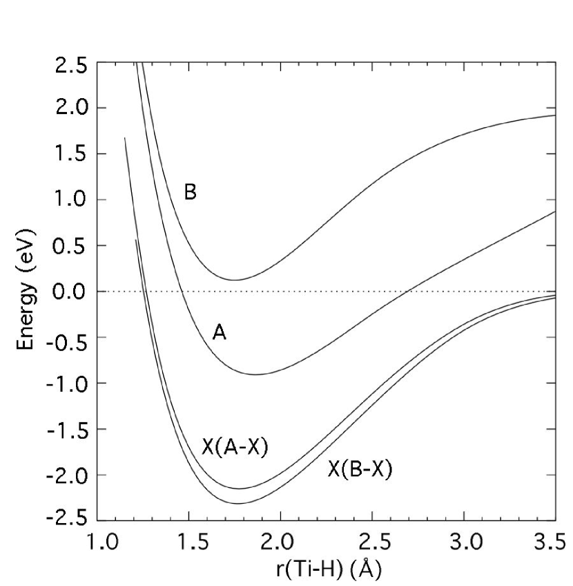
Figure 1: The core+valence IC-MRCI+Q potential energy curves for the $X$, $A$, and $B$ states. The zero of energy is Ti and H at infinite separation. The $X$ state is plotted twice, one curve is from the $A-X$ calculations while the second is from the B-X calculations. See the text for a full description of the two sets of calculations.

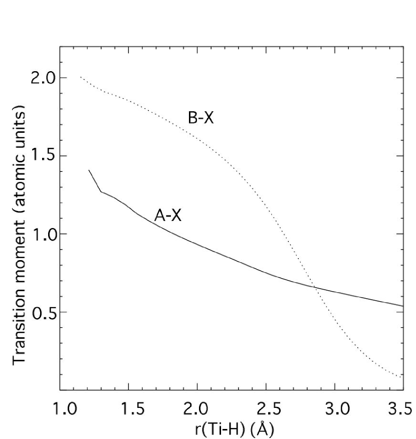
Figure 2: The core+valence IC-MRCI $A-X$ and $B-X$ transition dipole moments.

Given the limited experimental data it is difficult to definitively determine the best values for $\omega_{e}$, $\omega_{e}x_{e}$, and the transition moment. On the basis of previous calculation on CrH Bauschlicher et al. (2001); Burrows et al. (2002) and FeH Dulick et al. (2003), we feel that the calculations including the core+valence may yield superior values for all spectroscopic constants excluding the dipole moment, where the smaller active space used in the $B{}^{4}\Gamma-X{}^{4}\Phi$ calculations results in the valence treatment being superior for this property. For the $X{}^{4}\Phi$ state, we believe the results obtained using the $A{}^{4}\Phi-X{}^{4}\Phi$ treatment are superior because it has a larger active space and fewer states in the SA procedure. We also note that for the $A{}^{4}\Phi-X{}^{4}\Phi$ treatment, the $X$ state dipole moment improves when core correlation is included, which also supports using the $A{}^{4}\Phi-X{}^{4}\Phi$ treatment for the $X$ state. In the end, transition dipole moment functions computed at the core+valence level were used to generate the Einstein $A_{v^{\prime}v^{\prime\prime}}$ values for the $B{}^{4}\Gamma-X{}^{4}\Phi$ and $A{}^{4}\Phi-X{}^{4}\Phi$ transitions in Table 2. The transition moments and IC-MRCI+Q potentials used to compute the $A$ values in Table 2 are plotted in Figures 1 and 2, respectively.

Finally, we compare our best values to previous theoretical values. Our best results are in reasonable agreement with those reported by Anglada et al. (1990); for the $X$ and $A$ states their bond distances are 0.07 and 0.02 Å longer than our best values, respectively, and therefore in slightly worse agreement with experiment. Their $X$ state $\omega_{e}$ value is about 50 cm^-1 smaller than our best value, while their $A$ state value is about 140 cm^-1 larger than our best value. For the one bond distance for which they report their transition moments, their $A-X$ transition moment differs from our value by about 10%, while their $B-X$ moment is only very slightly smaller than our value. The $X$ state $r_{e}$ values reported by Koseki et al. (2002) are about 0.1 Å longer than our $r_{e}$ value. Their all electron $\omega_{e}$ value is in better agreement with our value than is their value with scalar relativistic effects added. This is a bit surprising since our calculations include the scalar relativistic effects. Overall the agreement between the different theoretical approaches is relatively good. Our use of much larger basis sets and the inclusion of core-valence correlation results in bond lengths that are in better agreement with experiment, and we assume that the other spectroscopic properties are more accurate in our calculations as well.

4 LINE POSITIONS AND INTENSITIES

A common feature associated with the electronic structure of transition metal hydrides is that the excited electronic states are often heavily perturbed by unobserved neighboring states whereas the ground states are for the most part unperturbed. The $X^{4}\Phi$, $A^{4}\Phi$, and $B^{4}\Gamma$ states of TiH are no exception. Recent work on the analyses of high-resolution Fourier transform emission and laser excitation spectra of the $A^{4}\Phi-X^{4}\Phi$ (Andersson et al. 2003) and $B^{4}\Gamma-X^{4}\Phi$ (Steimle et al. 1991; Launila & Lindgren 1996) $0-0$ bands have finally yielded rotational assignments for the heavily perturbed $A$ and $B$ states.

As a prerequisite to calculating opacities for temperatures up to 2000 K, a synthesized spectrum was generated comprised of rovibrational line positions and Einstein $A$-values for quantum numbers up to $v^{\prime\prime}=v^{\prime}=5$ and $J^{\prime\prime}=J^{\prime}=50.5$. Because the only available experimental data for these states is for $v=0$, we had to rely heavily on the ab initio calculations described above to supply the missing information on the vibrational structure. In particular, the first 4 vibrational levels were calculated from the ab initio potentials and fitted with 3 vibrational constants as reported at the end of Table 6. Note that the vibrational constants of Table 1 were generated in the same way but with 3 vibrational levels and 2 fitted vibrational constants (as listed in Table 1). The vibrational constants in Tables 1 and 6 are therefore slightly different.

The electronic coupling in the $X$, $A$, and $B$ states is intermediate Hund’s case (a) – (b) over a wide range of $J$. The case (a) Hamiltonians for the ${}^{4}\Phi$ and ${}^{4}\Gamma$ states in Tables 3 and 4, respectively, were selected for least-squares fitting of the experimental data. In determining the molecular constants for the $X$ state, the reported rotational lines in Andersson et al. (2003) were reduced to lower state combination differences, yielding the molecular constants listed in Table 5. ¿From these fitted constants, the $X$ state term energies were calculated and then used in transforming the observed rotational lines in the $A-X$ and $B-X$ $0-0$ bands into term energies for the $A$ and $B$ states. Molecular constants derived from fits of the $A$ and $B$ term energies are also listed in Table 5.

Except for the $X$ state, the centrifugal constants $D_{0}$ and $H_{0}$ were not statistically determined. Instead, these constants were held fixed in the fits of the $A$ and $B$ states to the values determined by the Dunham approximations,

$$D_{v} \simeq \xi^{2}B_{v}\hskip 10.0pt\mbox{and}\hskip 10.0ptH_{v}\>\simeq\>\xi^{5}\omega_{e}-\xi^{3}\alpha_{e}/3$$ (1)

where $\xi=2B_{v}/\omega_{e}$ and estimated values for $\omega_{e}$ and $\alpha_{e}$ were supplied by our ab initio calculations (Table 6). The presence of an anomalously large $e/f$ parity splitting in the $A$ state, undoubtedly due to perturbations, required separate fits of the $e$- and $f$-parity term energies, yielding the two sets of molecular constants in Table 5. Finally, the standard deviations from the fits, 0.031, 0.28, 0.16, and 1.18 cm^-1 for the $X$, $A$(e), $A$(f), and $B$ states, are comparable in quality to 0.026 and 0.42 cm^-1 for $X$ and $A$ (Andersson et al. 2003) and 0.020 and 0.573 cm^-1 for $X$ and $B$ (Launila & Lingren 1996) with roughly the same number of data points and adjustable parameters.

The molecular constants for $v>0$ were generated in a straightforward manner. With the ab initio estimates, $\omega_{e}$, $\omega_{e}x_{e}$, $\omega_{e}y_{e}$, $\alpha_{e}$, $\gamma_{e}$, and $\epsilon_{e}$, for each state (Table 6), the rotational constants for $v>0$ were computed from

$$B_{v} = B_{e}-\alpha_{e}(v+1/2)+\gamma_{e}(v+1/2)^{2}+\epsilon_{e}(v+1/2)^{3}$$ (2)

where the $B_{e}$’s were determined from $B_{0}$’s, the centrifugal constants $D_{v}$ and $H_{v}$ from eq. (1), and the spin-component energies $T_{v}(\Omega)$ by starting from the $T_{0}(\Omega)$ values and recursively adding vibrational separations of

$$\Delta G(v) = \omega_{e}-2v\>\omega_{e}x_{e}+(3v^{2}+1/4)\>\omega_{e}y_{e}$$ (3)

for $v>0$ in which the dependence of $A$, $\lambda$, and $\gamma$ on $v$ was assumed to be negligible. The list of molecular constants in Table 6 were then used with the ${}^{4}\Phi$ and ${}^{4}\Gamma$ Hamiltonians in computing the term energies from $v=0$ to $v=5$ for $e/f$ rotational levels up to $J=50.5$ for the $X$, $A(e)$, $A(f)$, and $B$ states. Note that all of the vibrational constants have been obtained using ab initio calculations so the location of bands with $\Delta v\not=0$ (computed using equation (3)) is relatively uncertain.

In our calculations the Einstein $A$-value is partitioned as

$$A = A_{v^{\prime}v^{\prime\prime}}\>\mbox{HLF}/(2J^{\prime}+1)$$

where $A_{v^{\prime}v^{\prime\prime}}$ is the Einstein $A$ for the vibronic transition $v^{\prime}-v^{\prime\prime}$, calculated using the ab initio electronic transition dipole moment function, and HLF is the Hönl–London factor. For reference, the Hönl-London factors (labeled as $S(J)$) in Tables 7 – 10 for ${}^{4}\Phi-{{}^{4}\Phi}$ and ${}^{4}\Gamma-{{}^{4}\Phi}$ transitions involving pure Hund’s case (a) and (b) coupling were derived using the method discussed in Dulick et al. (2003). Because the coupling in the $X$, $A$, and $B$ states is intermediate Hund’s case (a) – (b), the actual HLF’s were computed by starting from $\mbox{\bf{U}}^{\dagger}_{l}\mbox{\bf{T}}\mbox{\bf{U}}_{u}$, where $\mbox{\bf{U}}_{l}$ and $\mbox{\bf{U}}_{u}$ are the eigenvectors obtained from the diagonalizations of the lower and upper state Hamiltonians and T is the electric-dipole transition matrix (cf., eq. (1) in Dulick et al. (2003)). Squaring the matrix elements of $\mbox{\bf{U}}^{\dagger}_{l}\mbox{\bf{T}}\mbox{\bf{U}}_{u}$ yield numbers proportional to the HLF’s for intermediate coupling. In the absence of perturbations from neighboring states, as $J$ becomes large, the intermediate case HLF’s asymptotically approach the pure Hund’s case (b) values.

5 CHEMICAL ABUNDANCES OF TITANIUM HYDRIDE

In order to estimate the contribution ${\rm TiH}$ makes to M dwarf spectra, its abundance must be calculated. This is accomplished by minimizing the total free energy of the ensemble of species using the same methods as Sharp & Huebner (1990) and Burrows & Sharp (1999) (see Appendix A). To calculate the abundance of a particular species, its Gibbs free energy of formation from its constituent elements must be known. Using the new spectroscopic constants derived in §2 and §3, we have calculated for TiH this free energy and its associated partition function. In the case of ${\rm TiH}$, its dissociation into its constituent elements can be written as the equilibrium

$${\rm TiH}\rightleftharpoons{\rm Ti}+{\rm H}\,.$$

The Gibbs energy of formation is then calculated from eq. (A1) in Appendix A. Eq. (A1) is the general formula for obtaining the energy of formation of a gas-phase atomic or molecular species, be it charged or neutral.

Since the publication of Burrows & Sharp (1999), we have upgraded our chemical database significantly with the inclusion of several additional titanium-bearing compounds, and have updated most of the thermochemical data for titanium-bearing species (Barin 1995). In addition to ${\rm TiH}$, the new species are the solid condensates ${\rm TiS}$, ${\rm Mg_{2}TiO_{4}}$, ${\rm Ca_{3}Ti_{2}O_{7}}$, and ${\rm Ca_{4}Ti_{3}O_{10}}$, and the revised data are for the gas-phase species ${\rm TiO}$, TiO₂, and ${\rm TiS}$, the liquid condensates ${\rm TiN}$, ${\rm TiO_{2}}$, ${\rm Ti_{2}O_{3}}$, ${\rm Ti_{3}O_{5}}$, ${\rm Ti_{4}O_{7}}$, ${\rm MgTiO_{3}}$, ${\rm Mg_{2}TiO_{4}}$, and the solid condensates ${\rm TiN}$, ${\rm TiO_{2}}$, ${\rm Ti_{2}O_{3}}$, ${\rm Ti_{3}O_{5}}$, ${\rm Ti_{4}O_{7}}$, ${\rm MgTiO_{3}}$, ${\rm CaTiO_{3}}$, and ${\rm MgTi_{2}O_{5}}$. The revised data for TiO₂, in particular, have resulted in refined abundance estimates of TiO. We have obtained much better least-square fits to the free energy, and in nearly all cases the fitted polynomials agree to better than 10 cal mole^-1 compared with the tabulated values in Barin (1995) over the fitted temperature range, which for condensates corresponds to their stability field. For computational efficiency we sometimes extrapolate the polynomial fits of eq. (A2) for the condensates beyond the temperature range in which they are stable, but we ensure that the extrapolation is in a direction that further decreases stability.

Since ionization plays a significant role at higher temperatures, a number of ionized species are included in the gas phase, including electrons as an additional “element” with a negative stoichiometric coefficient. The ions considered in our equilibrium code are ${\rm e^{-}}$, ${\rm H^{+}}$, ${\rm H^{-}}$, ${\rm Li^{+}}$, ${\rm Na^{+}}$, ${\rm K^{+}}$, ${\rm Cs^{+}}$, ${\rm Mg^{+}}$, ${\rm Al^{+}}$, ${\rm Si^{+}}$, ${\rm Ti^{+}}$, ${\rm Fe^{+}}$, ${\rm H_{2}^{+}}$, ${\rm H_{2}^{-}}$, ${\rm OH^{+}}$, ${\rm CO^{+}}$, ${\rm NO^{+}}$, ${\rm N_{2}^{+}}$, ${\rm N_{2}^{-}}$, and ${\rm H_{3}O^{+}}$. Ions were not considered in the earlier work of Burrows and Sharp (1999).

The partition function of ${\rm TiH}$ is obtained from the estimated spectroscopic constants in Tables 11 and 12 (data taken from Table 1 and Anglada et al. 1990, or simply guessed). Table 11 lists 15 electronic states, with the quartet $X^{4}\Phi$ ground state being resolved into each of the four separate spin substates. The partition function is calculated using the method of Dulick et al. (2003). The contribution to the total partition function of each electronic state is determined using asymptotic approximations from the vibrational and rotational constants in Table 12, then these contributions are summed according to eq. (7) in Dulick et al. (2003), with the Boltzmann factor for the electronic energy being applied to each state, where the electronic energy of the lowest spin substate of the ground $X$ electronic state is zero by definition. Since the separate electronic energies for the spin substates of the ground electronic state are available, the $X$ state is treated as four separate states in the summation, so that effectively the sum is over 18 states. The partition function of titanium is obtained by summing over the term values below 20,000 cm^-1, with degeneracies as listed in Moore (1949). The partition function of hydrogen is set to a value of 2 for all the temperatures considered. Table 13 lists our resulting TiH partition function in steps of 200 K from 1200 K to 4800 K. Using the partition functions of ${\rm TiH}$, ${\rm Ti}$, and ${\rm H}$ in eq. (A1), $\Delta G(T)$ is calculated at 100 K intervals over the temperature range required to compute the abundance of ${\rm TiH}$, fitted to a polynomial, and then incorporated into our database.

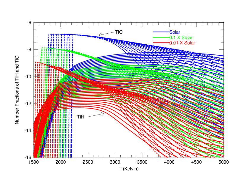
Figure 3: The log (base 10) of the number fractions of both TiH (solid) and TiO (dashed) as a function of temperature (T) from 1500 to 5000 Kelvin, for pressures from 10^-2 atmospheres to 10² atmospheres in equal logarithmic steps. Pressure increases for a given sequence from bottom to top. Furthermore, the condensation lines march rightward as the pressure increases. The abundances of both species are given for solar metallicity (blue), $0.1\times$ solar metallicity (green), and $0.01\times$ solar metallicity (red). TiO generally dominates at lower temperatures, until titanium condensables, such as perovskite, form, after which the abundances of all titanium compounds decrease precipitously (left of diagram). The condensation temperature increases with increasing pressure. However, at high temperatures, TiH comes into its own and its abundance can exceed that of TiO. For a given pressure, the temperature above which the TiH/TiO ratio exceeds unity is an increasing function of metallicity, being at 10² atmospheres and solar metallicity $\sim$4500 K, but at 10² atmospheres and $0.01\times$ solar metallicity $\sim$2500 K. As metallicity decreases, TiH becomes more and more important, though the abundances of both TiO and TiH decrease with metallicity. When the first titanium-bearing condensate appears, the abundance of TiH is already falling. Note that with increasing pressure the peak in TiH abundance shifts to higher temperatures more rapidly than the condensation temperature.

The thermochemistry indicates that the most important species of titanium are ${\rm TiO}$, ${\rm TiO_{2}}$, ${\rm TiH}$, ${\rm Ti}$, and ${\rm Ti^{+}}$. ${\rm TiO_{2}}$ is always subdominant and ${\rm Ti}$ and ${\rm Ti^{+}}$ are important only at higher temperatures than obtain in M, L, or T dwarf atmospheres. At solar metallicity, just before the first titanium-bearing condensate appears, ${\rm TiO_{2}}$ replaces Ti as the second most abundant titanium-bearing species, reaching an abundance of $\sim$9%. Figure 3 depicts the dependence of the TiO and TiH abundances with temperature from 1500 K to 5000 K for a range of pressures ($P$) from 10^-2 atmospheres to 10² atmospheres. This figure also shows the metallicity dependence of the TiO and TiH abundances. For solar metallicity, TiO dominates at low pressures below $\sim$4000 K and at high pressures below $\sim$4500 K, but the TiH abundances are not small. For solar metallicity, the TiH/TiO ratio at 10^-2 atmospheres and 2500 K is 10^-4 and at 10² atmospheres and 2500 K it is $\sim$10^-2 (one percent). The predominance of ${\rm TiO}$ before condensation, then its disappearance with condensation, matches the behavior seen in the M to L dwarf transition.

However, the abundance of TiO is a more strongly decreasing function of temperature than is that of TiH. For a given pressure, there is a temperature above which the TiH/TiO ratio actually goes above one. As Fig. 3 indicates, this transition temperature decreases with decreasing metallicity. For 0.01$\times$ solar metallicity and a pressure of 1 atmosphere, the TiH/TiO ratio hits unity at only $\sim$3500 K and at 10² atmospheres it does so near 2500 K. As a result, we expect that TiH will assume a more important role in low-metallicity subdwarfs than in “normal” dwarfs, with metallicities near solar. This fact is in keeping with the putative measurement of the TiH band near 0.94 $\mu$m (§6) in the subdwarf 2MASS J0532.

As expected, the abundance of gas-phase species containing titanium drops rapidly when the first titanium-bearing condensates appear, which occurs for solar metallicity at temperatures between 2200 K and 1700 K for pressures of 10² and 10^-2 atmospheres, respectively (see Fig. 3). At solar metallicity, when titanium-bearing condensates form, the TiH abundance is already falling with decreasing temperature; at condensation its abundance is at least an order of magnitude down from its peak abundance. As Fig. 3 indicates, the TiH abundance is an increasing function of pressure, but assumes a peak, sometimes broad, between the formation of condensates at lower temperatures and the formation of atomic Ti/Ti⁺ at higher temperatures.

The only significant previous study that included TiH is that of Hauschildt et al. (1997). These authors present numerical data in the form of fractional abundances in the gas phase for a number of titanium-bearing species, including TiO and TiH, as a function of optical depth. Unfortunately, this makes comparison with our results difficult. Nevertheless, we can still see that for their two solar-metallicity models the maximum ratio of the abundance of TiH to TiO is smaller than we obtain, sometimes by large factors. For instance, for their T_eff=2700 K model, at an optical depth of unity, their ${\rm TiH}$ abundance is over four orders of magnitude lower than that of TiO, and at an optical depth of 100, it is still down by three orders of magnitude. For their T_eff=4000 K model at unit optical depth, their ${\rm TiH}$ abundance is below that of TiO by three orders of magnitude. These very low abundances are in contrast to what we obtain at comparable $T/P$ points (cf. Fig. 3).

On the other hand, we find at a temperature of 2700 K, a pressure of 100 atmospheres, and solar metallicity that the abundance of TiH is as high as $\sim$1.5% of that of TiO. At 1 atmosphere, this ratio has dropped by about a factor of 10, but is still about a factor of 10 larger than the corresponding ratio in Hauschildt et al. At a temperature of 4000 K, a pressure of 100 atmospheres, and solar metallicity, we obtain a TiH/TiO abundance ratio as large as $\sim$24%. Furthermore, as previously mentioned, we find that the TiH/TiO ratio can go above one and at low metallicities is above one for a wider temperature range. Even at temperatures where this ratio is significantly below one, we conclude that the TiH abundance derived with the new thermochemical data is much higher than previously estimated.

6 TITANIUM HYDRIDE ABSORPTION OPACITIES

Using the results of §2, §3, and §4, we calculate the opacity of the two electronic systems $A^{4}\Phi-X^{4}\Phi$ and $B^{4}\Gamma-X^{4}\Phi$ of ${\rm TiH}$. These have band systems centered near 0.94 $\mu$m in the near IR and 0.53 $\mu$m in the visible, respectively. For the $A-X$ system, 4556 vibration-rotation transitions are considered for each of the 20 vibrational bands $v^{\prime}-v^{\prime\prime}$ with $v^{\prime}$=0 to 4 and $v^{\prime\prime}$=0 to 3, giving 91120 lines in total. For the $B-X$ system, 4498 vibration-rotation transitions are incorporated for each of the 24 vibrational bands $v^{\prime}$=0 to 3 and $v^{\prime\prime}$=0 to 5, giving 107,952 lines in total.

We use the same methods to calculate the line strengths and broadening as in §5 of Dulick et al. (2003), using the partition function of TiH from §5. Since broadening parameters for TiH are not available, those of ${\rm FeH}$ are used. In the absence of any other data, since ${\rm TiH}$ shares many characteristics with FeH, this is probably a reasonable assumption. A truncated Lorentzian profile is used, where the absorption in the wings of each line is truncated at min(25$\times P_{tot}$,100) cm^-1 on either side of the line center, $P_{tot}$ is the total gas pressure in atmospheres, and the detuning at which the absorption is set to zero does not exceed 100 cm^-1. To conserve the total line strength, the absorption in the part of the profile calculated is increased to account for the truncated wings. The reason for truncating the profiles is that we have no satisfactory theory to deal with the far wings of molecular lines, but we know that for atomic lines there is a rapid fall-off in the far wings, and, hence surmise that a rapid fall-off is probably realistic. However, our choice of determining its location is rather arbitrary.

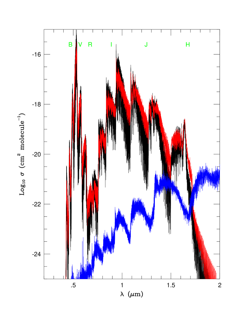
Figure 4: The log (base 10) of $\sigma$, the absorption cross section per molecule in cm², for ${\rm TiH}$ at 10 atmospheres and 3000 K (red) and 1 atmosphere and 2000 K (black). For comparison, the cross section per molecule for ${\rm H_{2}O}$ at 10 atmospheres and 3000 K is shown in blue. The approximate positions of the photometric bands $B$, $V$, $R$, $I$, $J$, and $H$ are also indicated. The broad absorption of ${\rm TiH}$ with several peaks between $\sim$0.7 $\mu$m and $\sim$1.95 $\mu$m is due to the $A-X$ electronic band system, and the absorption between $\sim$0.43 $\mu$m and $\sim$0.7 $\mu$m is due to the $B-X$ electronic band system. See text for a detailed discussion.

As with FeH, different isotopic versions are included in the calculations. The main isotope of ${\rm Ti}$ is ${\rm{}^{48}Ti}$, which makes up 73.8% of terrestrial titanium. The other isotopes of titanium are ${\rm{}^{46}Ti}$, ${\rm{}^{47}Ti}$, ${\rm{}^{49}Ti}$, and ${\rm{}^{50}Ti}$ with isotopic abundances of 8%, 7.3%, 5.5%, and 5.4%, respectively. Using the same methods as Dulick et al. (2003) based on Herzberg (1950), the shift in the energy levels, and, hence, the transition frequencies for the minor isotopic versions of TiH are calculated. As in the case of Dulick et al., the change in the line strength with isotope depends only on the isotopic fraction of Ti in that particular isotopic form, and effects due to changes in the partition function, Boltzmann factor, and intrinsic line strength are small, and so are neglected. Figure 4 shows the absorption opacity in cm² per ${\rm TiH}$ molecule (plotted in red) between a wavelength of 0.3 $\mu$m and 2.0 $\mu$m , at temperature/pressure points of 3000 K/10 atmospheres and 2000 K/1 atmosphere. For comparison, the ${\rm H_{2}O}$ (blue) opacities per molecule at 3000K and 10 atmospheres are also shown. The approximate location of the photometric bands $B$, $V$, and $R$ in the visible, and $I$, $J$, and $H$ in the infrared are also indicated.

The absorption spectrum of ${\rm TiH}$ covering the region in the near infrared from $\sim$0.7 $\mu$m (the limit of the far visible red) to $\sim$1.95 $\mu$m , is due to the $A-X$ electronic system, and the absorption between $\sim$0.43 $\mu$m and $\sim$0.7 $\mu$m in the visible is due to the $B-X$ electronic system. The two electronic systems overlap at $\sim$0.7 $\mu$m . The strongest absorption in the $A-X$ system corresponds to the $\Delta v$=0 bands (0-0, 1-1, 2-2, etc.), the next strongest peaks at a shorter wavelength and corresponds to the $\Delta v=1$ bands (1-0, 2-1, 3-2, etc.), and the next strongest peaks at a longer wavelength and corresponds to the $\Delta v=-1$ bands (0-1, 1-2, 2-3, etc.). There is a similar structure for the $B-X$ system. Many of the peak absorption features of TiH occur at about the same wavelengths as the peaks in absorption of ${\rm TiO}$, which is more abundant. This is particularly obvious for the $A-X$ system of ${\rm TiH}$. Moreover, although the cross section per molecule of ${\rm H_{2}O}$ is much less than that of ${\rm TiH}$ over most of the wavelength region, ${\rm H_{2}O}$ is far more abundant, and the five peaks corresponding to the $\Delta v$=-2, -1, 0, 1 and 2 sequence of bands for this $A-X$ system of TiH match up approximately with peaks in the ${\rm H_{2}O}$ absorption spectrum.

Therefore, because of the particular wavelength positions of the ${\rm TiO}$ and ${\rm H_{2}O}$ absorption bands and the high abundances of the ${\rm TiO}$ and ${\rm H_{2}O}$ molecules at solar metallicity, identifying ${\rm TiH}$ in a solar-metallicity M or L dwarf spectrum, while not impossible, is likely to be difficult. However, the TiH features are not completely obscured, in particular at $\sim$0.52 $\mu$m , $\sim$0.94 $\mu$m , and weakly in the $H$ band near 1.6 $\mu$m . Notice that the band heads of the $A-X$ transition are mainly R-heads because $B^{\prime}<B^{\prime\prime}$ but for the $\Delta v=-3$ sequence in the $H$ band the shading changes and P-heads form. The peak in the ${\rm TiH}$ absorption in the $H$ band corresponds with a deep trough of the ${\rm TiO}$ absorption, and is close to a minimum in the ${\rm H_{2}O}$ absorption. Therefore, in particular in subdwarfs with sub-solar metallicities, for which the abundances of metal hydrides come into their own vis à vis metal oxides (Fig. 3), spectral features of TiH in the $H$ band and at 0.94 $\mu$m should emerge. The larger TiH abundances we derive in §5 also suggest this. The recent detection in the subdwarf L dwarf 2MASS J0532 by Burgasser, Kirkpatrick & Lépine (2004) of the TiH feature at 0.94 $\mu$m is in keeping with these expectations.

7 CONCLUSIONS

For the TiH molecule, we have combined ab initio calculations with spectroscopic measurements to derive new thermochemical data, new spectral line lists and oscillator strengths, its abundance (for a given composition, temperature, and pressure), and its per-molecule absorption opacities. We find that with the new partition functions, the abundance of TiH in M and L dwarf atmospheres is much higher than previously thought, that the TiH/TiO ratio increases strongly with decreasing metallicity, and that at high enough temperatures the TiH/TiO ratio can exceed unity. Furthermore, we conclude that, particularly for subdwarf L and M dwarfs, spectral features of TiH near 0.94 $\mu$m and in the $H$ band may not be weak. The recent putative detection of the 0.94 $\mu$m feature in the L subdwarf 2MASS J0532 is encouraging in this regard and suggests that the detection of TiH in other dwarfs may shed light on their atmospheric titanium chemistry.

Appendix A FREE ENERGY OF A GAS-PHASE SPECIES

The Gibbs free energy of formation of any gas-phase species, relative to its constituent element or elements in their monatomic gaseous state, can be calculated if its spectroscopic data, and those of its constituent elements, are known. We start with the equilibrium

$$Y^{q}+q{\rm e^{-}}\rightleftharpoons\sum_{i=1}^{j}n_{i}X_{i}\,,$$

where $Y$ represents an atomic or molecular species, and has the electric charge $q$, which is zero for a neutral species, $X_{i}$ represents the $i$-th element in $Y$, $n_{i}$ is the corresponding stoichiometric coefficient, $j$ is the number of different elements in $Y$, and ${\rm e^{-}}$ is the electron.

Based on a generalization of the Saha equation and the law of mass action, the following equation can be derived to obtain the Gibbs energy of formation of $Y^{q}$:

$$\Delta G(Y^{q})=-RT\Biggl{[}\ln\left(Q[Y^{q}]\right)-\sum_{i=1}^{j}n_{i}\ln\left(Q[X_{i}]\right)+\frac{hcE}{kT}+\frac{5}{2}(1+q-N)\ln T$$

$$+\frac{3}{2}\Biggl{\{}\ln\left(\sum_{i=1}^{j}n_{i}m_{i}\right)-qm_{e}\Biggr{\}}+q\left(\ln 2+\frac{3}{2}\ln m_{e}\right)$$

$$+(1+q+N)\biggl{\{}\frac{5}{2}\ln k+\frac{3}{2}\ln\left[\frac{2\pi}{N_{A}h^{2}}\right]-\ln A_{o}\biggr{\}}\Biggr{]}\,,$$ (A1)

where $Q[Y^{q}]$ and $Q[X_{i}]$ are the partition functions corresponding to $Y^{q}$ and the atoms $X_{i}$, respectively, and $E$ is the total energy (in wavenumbers) to fully dissociate a neutral molecule into its constituent atoms, if the species is a molecule. For a positive ion, the ionization potential (or, for a multiply charged positive ion, the sum of the ionization potentials) must be included in $E$. For a negative ion, the electron affinity must be subtracted from $E$. In addition, the total number of atoms in the molecule is $N$, and is given by $\sum_{i=1}^{j}n_{i}$, i.e., the sum of the number of atoms of each element over the number of elements. The mass of the electron and the mass of the $i$-th element are $m_{e}$ and $m_{i}$ in amu, respectively, $R$, $N_{A}$, and $A_{o}$ are the gas constant, Avogadro’s number, and the standard atmosphere, respectively, and the other symbols have their usual meanings.

To be rigorously correct, for ions the molecular weight is corrected for the gain/loss in mass due to the addition/removal of electrons. For neutral monatomic species all terms on the right hand side of eq. (A1) cancel yielding zero, and the energy of formation for free electrons is zero by definition. For convenience, all the temperature-independent terms (after multiplying by $-RT$) have been collected together, and depend only on the mass, the number of atoms, and charge of the species.

In order to incorporate the free energies into our existing database in a uniform way, eq. (A1) is calculated at 100 K intervals over the temperature range we are likely to use, then a polynomial fit of the form

$$\Delta G(T)=a/T+b+cT+dT^{2}+eT^{3}$$ (A2)

is made. The lowest number of coefficients that make the best fit over the calculated range is adopted. The results for TiH using this procedure are $a$=-3.046$\times 10^{5}$, $b$=-4.915$\times 10^{4}$, $c$=2.325$\times 10^{1}$, $d$=-1.568$\times 10^{-4}$, and $e$=4.539$\times 10^{-8}$ for $G(T)$ in calories per mole.

In the case of diatomic neutral molecules, such as ${\rm TiH}$, eq. (A1) simplifies by putting $q=0$, $N=2$, $j=2$ and $n_{1}=n_{2}=1$, and the appropriate partition functions for the molecule and the atoms are used. In addition, the energy $E$ to fully dissociate the molecule is just the dissociation potential from the ground vibrational level of the ground electronic state, which for ${\rm TiH}$ is 2.08 eV, or 16776 cm^-1.

Table 1: Summary of IC-MRCI+Q Spectroscopic Constants.

State	$r_{0}$(Å)	$\omega_{e}$(cm-1)	$\omega_{e}x_{e}$(cm-1)	Dipole(debye)a	$T_{00}$(cm-1)
valence correlation
$A{}^{4}\Phi-X{}^{4}\Phi$ calculation
$X{}^{4}\Phi$	1.818	1533.4	21.94	2.30	0
$A{}^{4}\Phi$	1.896	1375.9	23.17	2.81	10745
$B{}^{4}\Gamma-X{}^{4}\Phi$ calculation
$X{}^{4}\Phi$	1.821	1527.0	21.85	2.13	0
${}^{4}\Pi$	1.838	1489.3	22.31	1.91	1694
${}^{4}\Delta$	1.905	1402.4	21.82	1.17	4082
$B{}^{4}\Gamma$	1.804	1577.8	27.52	3.19	17735
core+valence correlation
$A{}^{4}\Phi-X{}^{4}\Phi$ calculation
$X{}^{4}\Phi$	1.788	1548.9	20.23	2.46	0
$A{}^{4}\Phi$	1.888	1342.6	21.26	3.25	11237
$B{}^{4}\Gamma-X{}^{4}\Phi$ calculation
$X{}^{4}\Phi$	1.794	1529.2	20.04	1.52b	0
${}^{4}\Pi$	1.813	1487.4	20.36	1.40	1732
${}^{4}\Delta$	1.885	1398.7	20.66	1.24	4231
$B{}^{4}\Gamma$	1.764	1592.5	27.07	2.59	18874
Experiment
$X{}^{4}\Phi$	1.779c	1385.3d		2.455e	0
$A{}^{4}\Phi$	1.867c				10595c
$B{}^{4}\Gamma$	1.7248f			2.998e	18878f

^a Computed as an expectation value at the IC-MRCI level.

^b Using a finite field approach, the IC-MRCI(+Q) level yields 2.06(2.17)debye.

^c Andersson et al. (2003). Note Launila & Lindgren (1996) give 1.7847 Å for $r_{0}$ of the $X$ state.

^d Chertihin & Andrews (1994).

^e Steimle et al. (1991).

^f Launila & Lindgren (1996).

Table 2: Einstein A${}_{v^{\prime}v^{\prime\prime}}$ Values for the Bands of the $B{}^{4}\Gamma-X{}^{4}\Phi$ and $A{}^{4}\Phi-X{}^{4}\Phi$ Transitions.

v′	v′′	A (s-1) [$B{}^{4}\Gamma-X{}^{4}\Phi$]	A (s-1) [$A{}^{4}\Phi-X{}^{4}\Phi$   ]
0	0	0.4003$\times 10^{8}$	0.2336$\times 10^{7}$
0	1	0.6103$\times 10^{6}$	0.7567$\times 10^{6}$
0	2	0.1279$\times 10^{5}$	0.1776$\times 10^{6}$
0	3	0.2072$\times 10^{3}$	0.3919$\times 10^{5}$
0	4	0.7146	-
0	5	0.2469	-
1	0	0.3239$\times 10^{6}$	0.2577$\times 10^{6}$
1	1	0.3831$\times 10^{8}$	0.1329$\times 10^{7}$
1	2	0.1105$\times 10^{7}$	0.1071$\times 10^{7}$
1	3	0.3751$\times 10^{5}$	0.4074$\times 10^{6}$
1	4	0.9085$\times 10^{3}$	-
1	5	0.6571$\times 10^{1}$	-
2	0	0.1205$\times 10^{4}$	0.8251$\times 10^{4}$
2	1	0.5105$\times 10^{6}$	0.4106$\times 10^{6}$
2	2	0.3664$\times 10^{8}$	0.6651$\times 10^{6}$
2	3	0.1463$\times 10^{7}$	0.1090$\times 10^{7}$
2	4	0.7186$\times 10^{5}$	-
2	5	0.2383$\times 10^{4}$	-
3	0	0.2718$\times 10^{3}$	0.9007$\times 10^{2}$
3	1	0.8623$\times 10^{4}$	0.2273$\times 10^{5}$
3	2	0.5489$\times 10^{6}$	0.4793$\times 10^{6}$
3	3	0.3499$\times 10^{8}$	0.4793$\times 10^{6}$
3	4	0.1664$\times 10^{7}$	-
3	5	0.1119$\times 10^{6}$	-
4	0	-	0.2572
4	1	-	0.3647$\times 10^{3}$
4	2	-	0.4142$\times 10^{5}$
4	3	-	0.4816$\times 10^{6}$

Table 3: ${}^{4}\Phi$ Hund’s Case (a) Hamiltonian Matrix

$x=J+1/2$, $t=\sqrt{3(x^{2}-4)}$, $u=\sqrt{4(x^{2}-9)}$, $v=\sqrt{3(x^{2}-16)}$
$\displaystyle{\begin{array}[]{r@{\hspace{5pt}}c@{\hspace{5pt}}l}T(9/2)\hskip 5.0&=\hfil\hskip 5.0&T+9A/2+2\lambda+3\gamma\\[5.0pt] T(7/2)\hskip 5.0&=\hfil\hskip 5.0&T+3A/2-2\lambda-2\gamma\\[5.0pt] T(5/2)\hskip 5.0&=\hfil\hskip 5.0&T-3A/2-2\lambda-5\gamma\\[5.0pt] T(3/2)\hskip 5.0&=\hfil\hskip 5.0&T-9A/2+2\lambda-6\gamma\\[5.0pt] \end{array}}$
$<9/2|H|9/2>$	=	$T(9/2)+(x^{2}-10)B-(x^{4}-17x^{2}+52)D+(x^{6}-21x^{4}+96x^{2}-40)H$
$<9/2|H|7/2>$	=	$<7/2|H|9/2>\>=\>-v\>[B-\gamma/2-2(x^{2}-5)D+(3x^{4}-23x^{2}+16)H]$
$<9/2|H|5/2>$	=	$<5/2|H|9/2>\>=\>-uv\>[D-(3x^{2}-4)H]$
$<9/2|H|3/2>$	=	$<3/2|H|9/2>\>=\>-tuvH$
$<7/2|H|7/2>$	=	$T(7/2)+x^{2}B-(x^{4}+7x^{2}-84)D+(x^{6}+21x^{4}-258x^{2}+264)H$
$<7/2|H|5/2>$	=	$<5/2|H|7/2>\>=\>-u\>[B-\gamma/2-2(x^{2}+3)D+(3x^{4}+28x^{2}-60)H]$
$<7/2|H|3/2>$	=	$<3/2|H|7/2>\>=\>-tu\>(D-(3x^{2}+14)H)$
$<5/2|H|5/2>$	=	$T(5/2)+(x^{2}+6)B-(x^{4}+19x^{2}-12)D+(x^{6}+39x^{4}+72x^{2}-456)H$
$<5/2|H|3/2>$	=	$<3/2|H|5/2>\>=\>-t\>[B-\gamma/2-2(x^{2}+7)D+(3x^{4}+49x^{2}+100)H]$
$<3/2|H|3/2>$	=	$T(3/2)+(x^{2}+8)B-(x^{4}+19x^{2}+52)D+(x^{6}+33x^{4}+222x^{2}+248)H$

Table 4: ${}^{4}\Gamma$ Hund’s Case (a) Hamiltonian Matrix

$x=J+1/2$, $t=\sqrt{3(x^{2}-25)}$, $u=\sqrt{4(x^{2}-16)}$, $v=\sqrt{3(x^{2}-9)}$
$\displaystyle{\begin{array}[]{r@{\hspace{5pt}}c@{\hspace{5pt}}l}T(11/2)\hskip 5.0&=\hfil\hskip 5.0&T+6A+2\lambda+9\gamma/2\\[5.0pt] T(9/2)\hskip 5.0&=\hfil\hskip 5.0&T+2A-2\lambda-3\gamma/2\\[5.0pt] T(7/2)\hskip 5.0&=\hfil\hskip 5.0&T-2A-2\lambda-11\gamma/2\\[5.0pt] T(5/2)\hskip 5.0&=\hfil\hskip 5.0&T-6A+2\lambda-15\gamma/2\end{array}}$
$<11/2|H|11/2>$	=	$T(11/2)+(x^{2}-13)B-(x^{4}-23x^{2}+94)D+(x^{6}-30x^{4}+201x^{2}-172)H$
$<11/2|H|9/2>$	=	$<9/2|H|11/2>\>=\>-t\>[B-\gamma/2-2(x^{2}-7)D+(3x^{4}-35x^{2}+44)H]$
$<11/2|H|7/2>$	=	$<7/2|H|11/2>\>=\>-tu\>[D-(3x^{2}-7)H]$
$<11/2|H|5/2>$	=	$<5/2|H|11/2>\>=\>-tuvH$
$<9/2|H|9/2>$	=	$T(9/2)+(x^{2}-1)B-(x^{4}+5x^{2}-138)D+(x^{6}+18x^{4}-439x^{2}+804)H$
$<9/2|H|7/2>$	=	$<7/2|H|9/2>\>=\>-u\>[B-\gamma/2-2(x^{2}+3)D+(3x^{4}+28x^{2}-123)H]$
$<9/2|H|5/2>$	=	$<5/2|H|9/2>\>=\>-uv\>[D-(3x^{2}+17)H]$
$<7/2|H|7/2>$	=	$T(7/2)+(x^{2}+7)B-(x^{4}+21x^{2}-42)D+(x^{6}+42x^{4}+x^{2}-1164)H$
$<7/2|H|5/2>$	=	$<5/2|H|7/2>\>=\>-v\>[B-\gamma/2-2(x^{2}+9)D+(3x^{4}+61x^{2}+156)H]$
$<5/2|H|5/2>$	=	$T(5/2)+(x^{2}+11)B-(x^{4}+25x^{2}+94)D+(x^{6}+42x^{4}+369x^{2}+548)H$

Table 5: Derived Molecular Constants (cm^-1) From Observed Data

State	$T_{0}$	$B_{0}$	$D_{0}\times 10^{4}$	$H_{0}\times 10^{9}$	$A_{0}$	$\gamma_{0}$
$X^{4}\Phi$	string85.1362	5.3668672(614)	2.61187(303)	string9.108(405)	32.96454(797)	string0.193432(889)
$A^{4}\Phi(e)$	10688.3028(848)	4.876910(846)	2.58010	–8.025	30.4589(246)	–0.10251(733)
$A^{4}\Phi(f)$	10687.880(156)	4.86282(109)	2.55780	–8.112	29.0992(410)	–0.22281(435)
$B^{4}\Gamma$	18799.595(238)	5.70361(115)	2.94312	–7.459	39.1548(442)	–1.0047(147)

Table 6: Generated Molecular Constants (cm^-1) for the $X\>^{4}\Phi$, $A\>^{4}\Phi$, and $B\>^{4}\Gamma$ Vibrational Levels

$v$	$B_{v}$	$D_{v}\times 10^{4}$	$H_{v}\times 10^{9}$	$T_{v}(\Lambda-3/2)$	$T_{v}(\Lambda-1/2)$	$T_{v}(\Lambda+1/2)$	$T_{v}(\Lambda+3/2)$
$X\>^{4}\Phi$ State
0	5.3668672	2.61187	string9.108	–64.3649	string34.7222	string134.1962	string234.0570
1	5.1007701	2.21602	–8.378	1444.1222	1543.2093	1642.6833	1742.5441
2	4.8611877	1.91820	–8.781	2912.1487	3011.2358	3110.7098	3210.5707
3	4.6513671	1.68039	–8.813	4338.4489	4437.5360	4537.0100	4636.8709
4	4.4745555	1.49595	–8.652	5721.7571	5820.8442	5920.3182	6020.1790
5	4.3340001	1.35936	–8.424	7060.8075	7159.8946	7259.3686	7359.2294
$A\>^{4}\Phi(e)$ State
0	4.8769102	2.58010	–8.025	10548.6548	10646.3250	10737.3941	10821.8623
1	4.6169393	2.18919	–9.213	11848.7691	11946.4393	12037.5085	12121.9766
2	4.3736732	1.86106	–9.643	13106.3657	13204.0358	13295.1050	13379.5732
3	4.1484432	1.58810	–9.585	14319.7104	14417.3805	14508.4497	14592.9179
4	3.9425804	1.36321	–9.237	15487.0692	15584.7394	15675.8086	15760.2767
5	3.7574161	1.18002	–8.745	16606.7082	16704.3784	16795.4476	16879.9157
$A\>^{4}\Phi(f)$ State
0	4.8628162	2.55780	–8.112	10547.0989	10656.5177	10743.1469	10806.9864
1	4.6028453	2.16921	–9.254	11847.2133	11956.6321	12043.2612	12107.1008
2	4.3595792	1.84313	–9.651	13104.8098	13214.2286	13300.8578	13364.6973
3	4.1343492	1.57197	–9.569	14318.1545	14427.5733	14514.2025	14578.0420
4	3.9284864	1.34864	–9.205	15485.5134	15594.9321	15681.5613	15745.4009
5	3.7433221	1.16679	–8.701	16605.1524	16714.5711	16801.2003	16865.0399
$B\>^{4}\Gamma$ State
0	5.7036054	2.94312	–7.459	18572.2017	18726.8115	18879.4119	19030.0029
1	5.4171527	2.52009	–8.938	20110.5248	20265.1346	20417.7350	20568.3260
2	5.1537792	2.17010	–9.613	21594.7116	21749.3214	21901.9218	22052.5128
3	4.9169618	1.88449	–9.772	23020.5977	23175.2075	23327.8079	23478.3989
4	4.7101772	1.65659	–9.636	24384.0185	24538.6283	24691.2287	24841.8197
5	4.5369023	1.48041	–9.363	25680.8094	25835.4192	25988.0196	26138.6106

Table 7: ${{}^{4}\Phi}-{{}^{4}\Phi}$ Hönl-London Factors – Case (a) Coupling

Branch	$\Omega^{\prime\prime}$	Parity	$\Omega^{\prime}$	Parity	$S(J)$
$P(J)$	9/2	$e/f$	9/2	$e/f$	$\displaystyle{\frac{1}{4}\cdot\frac{(2J-9)\>(2J+9)}{J}}$
$P(J)$	7/2	$e/f$	7/2	$e/f$	$\displaystyle{\frac{1}{4}\cdot\frac{(2J-7)\>(2J+7)}{J}}$
$P(J)$	5/2	$e/f$	5/2	$e/f$	$\displaystyle{\frac{1}{4}\cdot\frac{(2J-5)\>(2J+5)}{J}}$
$P(J)$	3/2	$e/f$	3/2	$e/f$	$\displaystyle{\frac{1}{4}\cdot\frac{(2J-3)\>(2J+3)}{J}}$
$Q(J)$	9/2	$e/f$	9/2	$f/e$	$\displaystyle{\frac{81}{4}\cdot\frac{2J+1}{J\>(J+1)}}$
$Q(J)$	7/2	$e/f$	7/2	$f/e$	$\displaystyle{\frac{49}{4}\cdot\frac{2J+1}{J\>(J+1)}}$
$Q(J)$	5/2	$e/f$	5/2	$f/e$	$\displaystyle{\frac{25}{4}\cdot\frac{2J+1}{J\>(J+1)}}$
$Q(J)$	3/2	$e/f$	3/2	$f/e$	$\displaystyle{\frac{9}{4}\cdot\frac{2J+1}{J\>(J+1)}}$
$R(J)$	9/2	$e/f$	9/2	$e/f$	$\displaystyle{\frac{1}{4}\cdot\frac{(2J-7)\>(2J+11)}{J+1}}$
$R(J)$	7/2	$e/f$	7/2	$e/f$	$\displaystyle{\frac{1}{4}\cdot\frac{(2J-5)\>(2J+9)}{J+1}}$
$R(J)$	5/2	$e/f$	5/2	$e/f$	$\displaystyle{\frac{1}{4}\cdot\frac{(2J-3)\>(2J+7)}{J+1}}$
$R(J)$	3/2	$e/f$	3/2	$e/f$	$\displaystyle{\frac{1}{4}\>\frac{(2J-1)\>(2J+5)}{J+1}}$

Table 8: ${{}^{4}\Phi}-{{}^{4}\Phi}$ Hönl-London Factors – Case (b) Coupling

Branch	$N^{\prime\prime}$	Parity	$N^{\prime}$	Parity	$S(J)$
${}^{P}P(J)$	$J-3/2$	$+/-$	$J-5/2$	$+/-$	$\displaystyle{\frac{1}{4}\cdot\frac{(2J-9)\>(2J+1)\>(2J+3)}{(2J-3)\>(J-1)}}$
${}^{Q}P(J)$	$J-3/2$	$+/-$	$J-3/2$	$+/-$	$\displaystyle{108\cdot\frac{2J+1}{J\>(2J-3)\>(2J-1)^{2}}}$
${}^{R}P(J)$	$J-3/2$	$+/-$	$J-1/2$	$+/-$	$\displaystyle{\frac{3}{4}\cdot\frac{(2J-7)\>(2J+5)}{J^{2}\>(2J-1)^{2}\>(J-1)}}$
${}^{P}P(J)$	$J-1/2$	$+/-$	$J-3/2$	$+/-$	$\displaystyle{\frac{1}{4}\cdot\frac{(2J-7)\>(2J-3)\>(2J+1)\>(2J+5)\>(J+1)}{J^{2}\>(2J-1)^{2}}}$
${}^{Q}P(J)$	$J-1/2$	$+/-$	$J-1/2$	$+/-$	$\displaystyle{576\cdot\frac{(J-1)\>(J+1)}{J\>(2J-1)^{2}\>(2J+1)^{2}}}$
${}^{R}P(J)$	$J-1/2$	$+/-$	$J+1/2$	$+/-$	$\displaystyle{\frac{3}{4}\cdot\frac{(2J-5)\>(2J+7)}{J^{2}\>(2J+1)^{2}\>(J+1)}}$
${}^{P}P(J)$	$J+1/2$	$+/-$	$J-1/2$	$+/-$	$\displaystyle{\frac{1}{4}\cdot\frac{(2J-5)\>(2J-1)\>(2J+3)\>(2J+7)\>(J-1)}{J^{2}\>(2J+1)^{2}}}$
${}^{Q}P(J)$	$J+1/2$	$+/-$	$J+1/2$	$+/-$	$\displaystyle{108\cdot\frac{2J-1}{J\>(2J+1)^{2}\>(2J+3)}}$
${}^{P}P(J)$	$J+3/2$	$+/-$	$J+1/2$	$+/-$	$\displaystyle{\frac{1}{4}\cdot\frac{(2J-3)\>(2J-1)\>(2J+9)}{(2J+3)\>(J+1)}}$
${}^{Q}Q(J)$	$J-3/2$	$+/-$	$J-3/2$	$+/-$	$\displaystyle{36\cdot\frac{(2J+1)\>(J+1)}{J\>(2J-1)^{2}}}$
${}^{R}Q(J)$	$J-3/2$	$+/-$	$J-1/2$	$+/-$	$\displaystyle{\frac{3}{4}\cdot\frac{(2J-7)\>(2J+1)\>(2J+5)}{J^{2}\>(2J-1)^{2}}}$
${}^{P}Q(J)$	$J-1/2$	$+/-$	$J-3/2$	$+/-$	$\displaystyle{\frac{3}{4}\cdot\frac{(2J-7)\>(2J+1)\>(2J+5)}{J^{2}\>(2J-1)^{2}}}$
${}^{Q}Q(J)$	$J-1/2$	$+/-$	$J-1/2$	$+/-$	$\displaystyle{36\cdot\frac{(2J^{2}+J-4)^{2}}{J\>(2J-1)^{2}\>(2J+1)\>(J+1)}}$
${}^{R}Q(J)$	$J-1/2$	$+/-$	$J+1/2$	$+/-$	$\displaystyle{\frac{1}{4}\cdot\frac{(2J-5)\>(2J-1)\>(2J+3)\>(2J+7)}{J^{2}\>(2J+1)\>(J+1)^{2}}}$
${}^{P}Q(J)$	$J+1/2$	$+/-$	$J-1/2$	$+/-$	$\displaystyle{\frac{1}{4}\cdot\frac{(2J-5)\>(2J-1)\>(2J+3)\>(2J+7)}{J^{2}\>(2J+1)\>(J+1)^{2}}}$
${}^{Q}Q(J)$	$J+1/2$	$+/-$	$J+1/2$	$+/-$	$\displaystyle{36\cdot\frac{(2J^{2}+3J-3)^{2}}{J\>(2J+1)\>(2J+3)^{2}\>(J+1)}}$
${}^{R}Q(J)$	$J+1/2$	$+/-$	$J+3/2$	$+/-$	$\displaystyle{\frac{3}{4}\cdot\frac{(2J-3)\>(2J+1)\>(2J+9)}{(2J+3)^{2}\>(J+1)^{2}}}$
${}^{P}Q(J)$	$J+3/2$	$+/-$	$J+1/2$	$+/-$	$\displaystyle{\frac{3}{4}\cdot\frac{(2J-3)\>(2J+1)\>(2J+9)}{(2J+3)^{2}\>(J+1)^{2}}}$
${}^{Q}Q(J)$	$J+3/2$	$+/-$	$J+3/2$	$+/-$	$\displaystyle{36\cdot\frac{J\>(2J+1)}{(2J+3)^{2}\>(J+1)}}$
${}^{R}R(J)$	$J-3/2$	$+/-$	$J-1/2$	$+/-$	$\displaystyle{\frac{1}{4}\cdot\frac{(2J-7)\>(2J+3)\>(2J+5)}{J\>(2J-1)}}$
${}^{Q}R(J)$	$J-1/2$	$+/-$	$J-1/2$	$+/-$	$\displaystyle{108\cdot\frac{2J+3}{(2J-1)\>(2J+1)^{2}\>(J+1)}}$
${}^{R}R(J)$	$J-1/2$	$+/-$	$J+1/2$	$+/-$	$\displaystyle{\frac{1}{4}\cdot\frac{(2J-5)\>(2J-1)\>(2J+3)\>(2J+7)\>(J+2)}{(2J+1)^{2}\>(J+1)^{2}}}$
${}^{P}R(J)$	$J+1/2$	$+/-$	$J-1/2$	$+/-$	$\displaystyle{\frac{3}{4}\cdot\frac{(2J-5)\>(2J+7)}{J\>(2J+1)^{2}\>(J+1)^{2}}}$
${}^{Q}R(J)$	$J+1/2$	$+/-$	$J+1/2$	$+/-$	$\displaystyle{576\cdot\frac{J\>(J+2)}{(2J+1)^{2}\>(2J+3)^{2}\>(J+1)}}$
${}^{R}R(J)$	$J+1/2$	$+/-$	$J+3/2$	$+/-$	$\displaystyle{\frac{1}{4}\cdot\frac{J\>(2J-3)\>(2J+1)\>(2J+5)\>(2J+9)}{(2J+3)^{2}\>(J+1)^{2}}}$
${}^{P}R(J)$	$J+3/2$	$+/-$	$J+1/2$	$+/-$	$\displaystyle{\frac{3}{4}\cdot\frac{(2J-3)\>(2J+9)}{(2J+3)^{2}\>(J+1)^{2}\>(J+2)}}$
${}^{Q}R(J)$	$J+3/2$	$+/-$	$J+3/2$	$+/-$	$\displaystyle{108\cdot\frac{2J+1}{(J+1)\>(2J+3)^{2}\>(2J+5)}}$
${}^{R}R(J)$	$J+3/2$	$+/-$	$J+5/2$	$+/-$	$\displaystyle{\frac{1}{4}\cdot\frac{(2J-1)\>(2J+1)\>(2J+11)}{(2J+5)\>(J+2)}}$

Table 9: ${{}^{4}\Gamma}-{{}^{4}\Phi}$ Hönl-London Factors – Case (a) Coupling

Branch	$\Omega^{\prime\prime}$	Parity	$\Omega^{\prime}$	Parity	$S(J)$
$P(J)$	9/2	$e/f$	11/2	$e/f$	$\displaystyle{\frac{1}{8}\cdot\frac{(2J-11)\>(2J-9)}{J}}$
$P(J)$	7/2	$e/f$	9/2	$e/f$	$\displaystyle{\frac{1}{8}\cdot\frac{(2J-9)\>(2J-7)}{J}}$
$P(J)$	5/2	$e/f$	7/2	$e/f$	$\displaystyle{\frac{1}{8}\cdot\frac{(2J-7)\>(2J-5)}{J}}$
$P(J)$	3/2	$e/f$	5/2	$e/f$	$\displaystyle{\frac{1}{8}\cdot\frac{(2J-5)\>(2J-3)}{J}}$
$Q(J)$	9/2	$e/f$	11/2	$f/e$	$\displaystyle{\frac{1}{8}\cdot\frac{(2J-9)\>(2J+1)\>(2J+11)}{J\>(J+1)}}$
$Q(J)$	7/2	$e/f$	9/2	$f/e$	$\displaystyle{\frac{1}{8}\cdot\frac{(2J-7)\>(2J+1)\>(2J+9)}{J\>(J+1)}}$
$Q(J)$	5/2	$e/f$	7/2	$f/e$	$\displaystyle{\frac{1}{8}\cdot\frac{(2J-5)\>(2J+1)\>(2J+7)}{J\>(J+1)}}$
$Q(J)$	3/2	$e/f$	5/2	$f/e$	$\displaystyle{\frac{1}{8}\cdot\frac{(2J-3)\>(2J+1)\>(2J+5)}{J\>(J+1)}}$
$R(J)$	9/2	$e/f$	11/2	$e/f$	$\displaystyle{\frac{1}{8}\cdot\frac{(2J+11)\>(2J+13)}{J+1}}$
$R(J)$	7/2	$e/f$	9/2	$e/f$	$\displaystyle{\frac{1}{8}\cdot\frac{(2J+9)\>(2J+11)}{J+1}}$
$R(J)$	5/2	$e/f$	7/2	$e/f$	$\displaystyle{\frac{1}{8}\cdot\frac{(2J+7)\>(2J+9)}{J+1}}$
$R(J)$	3/2	$e/f$	5/2	$e/f$	$\displaystyle{\frac{1}{8}\cdot\frac{(2J+5)\>(2J+7)}{J+1}}$

Table 10: ${{}^{4}\Gamma}-{{}^{4}\Phi}$ Hönl-London Factors – Case (b) Coupling

Branch	$N^{\prime\prime}$	Parity	$N^{\prime}$	Parity	$S(J)$
${}^{P}P(J)$	$J-3/2$	$+/-$	$J-5/2$	$+/-$	$\displaystyle{\frac{1}{8}\cdot\frac{(2J-11)\>(2J-9)\>(2J+1)}{(2J-3)\>(J-1)}}$
${}^{Q}P(J)$	$J-3/2$	$+/-$	$J-3/2$	$+/-$	$\displaystyle{\frac{3}{2}\cdot\frac{(2J-9)\>(2J+1)\>(2J+5)}{J\>(2J-3)\>(2J-1)^{2}}}$
${}^{R}P(J)$	$J-3/2$	$+/-$	$J-1/2$	$+/-$	$\displaystyle{\frac{3}{8}\cdot\frac{(2J+5)\>(2J+7)}{J^{2}\>(2J-1)^{2}\>(J-1)}}$
${}^{P}P(J)$	$J-1/2$	$+/-$	$J-3/2$	$+/-$	$\displaystyle{\frac{1}{8}\cdot\frac{(2J-9)\>(2J-7)\>(2J-3)\>(2J+1)\>(J+1)}{J^{2}\>(2J-1)^{2}}}$
${}^{Q}P(J)$	$J-1/2$	$+/-$	$J-1/2$	$+/-$	$\displaystyle{8\cdot\frac{(2J-7)\>(2J+7)\>(J-1)\>(J+1)}{J\>(2J-1)^{2}\>(2J+1)^{2}}}$
${}^{R}P(J)$	$J-1/2$	$+/-$	$J+1/2$	$+/-$	$\displaystyle{\frac{3}{8}\cdot\frac{(2J+7)\>(2J+9)}{J^{2}\>(2J+1)^{2}\>(J+1)}}$
${}^{P}P(J)$	$J+1/2$	$+/-$	$J-1/2$	$+/-$	$\displaystyle{\frac{1}{8}\cdot\frac{(2J-7)\>(2J-5)\>(2J-1)\>(2J+3)\>(J-1)}{J^{2}\>(2J+1)^{2}}}$
${}^{Q}P(J)$	$J+1/2$	$+/-$	$J+1/2$	$+/-$	$\displaystyle{\frac{3}{2}\cdot\frac{(2J-5)\>(2J-1)\>(2J+9)}{J\>(2J+1)^{2}\>(2J+3)}}$
${}^{P}P(J)$	$J+3/2$	$+/-$	$J+1/2$	$+/-$	$\displaystyle{\frac{1}{8}\cdot\frac{(2J-5)\>(2J-3)\>(2J-1)}{(2J+3)\>(J+1)}}$
${}^{Q}Q(J)$	$J-3/2$	$+/-$	$J-3/2$	$+/-$	$\displaystyle{\frac{1}{2}\cdot\frac{(2J-9)\>(2J+5)\>(2J+1)\>(J+1)}{J\>(2J-1)^{2}}}$
${}^{R}Q(J)$	$J-3/2$	$+/-$	$J-1/2$	$+/-$	$\displaystyle{\frac{3}{8}\cdot\frac{(2J+1)\>(2J+5)\>(2J+7)}{J^{2}\>(2J-1)^{2}}}$
${}^{P}Q(J)$	$J-1/2$	$+/-$	$J-3/2$	$+/-$	$\displaystyle{\frac{3}{8}\cdot\frac{(2J-9)\>(2J-7)\>(2J+1)}{J^{2}\>(2J-1)^{2}}}$
${}^{Q}Q(J)$	$J-1/2$	$+/-$	$J-1/2$	$+/-$	$\displaystyle{\frac{1}{2}\cdot\frac{(2J-7)\>(2J^{2}+J-4)^{2}\>(2J+7)}{J\>(2J-1)^{2}\>(2J+1)\>(J+1)}}$
${}^{R}Q(J)$	$J-1/2$	$+/-$	$J+1/2$	$+/-$	$\displaystyle{\frac{1}{8}\cdot\frac{(2J-1)\>(2J+3)\>(2J+7)\>(2J+9)}{J^{2}\>(2J+1)\>(J+1)^{2}}}$
${}^{P}Q(J)$	$J+1/2$	$+/-$	$J-1/2$	$+/-$	$\displaystyle{\frac{1}{8}\cdot\frac{(2J-7)\>(2J-5)\>(2J-1)\>(2J+3)}{J^{2}\>(2J+1)\>(J+1)^{2}}}$
${}^{Q}Q(J)$	$J+1/2$	$+/-$	$J+1/2$	$+/-$	$\displaystyle{\frac{1}{2}\cdot\frac{(2J-5)\>(2J^{2}+3J-3)^{2}\>(2J+9)}{J\>(2J+1)\>(2J+3)^{2}\>(J+1)}}$
${}^{R}Q(J)$	$J+1/2$	$+/-$	$J+3/2$	$+/-$	$\displaystyle{\frac{3}{8}\cdot\frac{(2J+1)\>(2J+9)\>(2J+11)}{(2J+3)^{2}\>(J+1)^{2}}}$
${}^{P}Q(J)$	$J+3/2$	$+/-$	$J+1/2$	$+/-$	$\displaystyle{\frac{3}{8}\cdot\frac{(2J-5)\>(2J-3)\>(2J+1)}{(2J+3)^{2}\>(J+1)^{2}}}$
${}^{Q}Q(J)$	$J+3/2$	$+/-$	$J+3/2$	$+/-$	$\displaystyle{\frac{1}{2}\cdot\frac{J\>(2J-3)\>(2J+1)\>(2J+11)}{(2J+3)^{2}\>(J+1)}}$
${}^{R}R(J)$	$J-3/2$	$+/-$	$J-1/2$	$+/-$	$\displaystyle{\frac{1}{8}\cdot\frac{(2J+3)\>(2J+5)\>(2J+7)}{J\>(2J-1)}}$
${}^{Q}R(J)$	$J-1/2$	$+/-$	$J-1/2$	$+/-$	$\displaystyle{\frac{3}{2}\cdot\frac{(2J-7)\>(2J+3)\>(2J+7)}{(2J-1)\>(2J+1)^{2}\>(J+1)}}$
${}^{R}R(J)$	$J-1/2$	$+/-$	$J+1/2$	$+/-$	$\displaystyle{\frac{1}{8}\cdot\frac{(2J-1)\>(2J+3)\>(2J+7)\>(2J+9)\>(J+2)}{(2J+1)^{2}\>(J+1)^{2}}}$
${}^{P}R(J)$	$J+1/2$	$+/-$	$J-1/2$	$+/-$	$\displaystyle{\frac{3}{8}\cdot\frac{(2J-7)\>(2J-5)}{J\>(2J+1)^{2}\>(J+1)^{2}}}$
${}^{Q}R(J)$	$J+1/2$	$+/-$	$J+1/2$	$+/-$	$\displaystyle{8\cdot\frac{J\>(2J-5)\>(2J+9)\>(J+2)}{(2J+1)^{2}\>(2J+3)^{2}\>(J+1)}}$
${}^{R}R(J)$	$J+1/2$	$+/-$	$J+3/2$	$+/-$	$\displaystyle{\frac{1}{8}\cdot\frac{J\>(2J+1)\>(2J+5)\>(2J+9)\>(2J+11)}{(2J+3)^{2}\>(J+1)^{2}}}$
${}^{P}R(J)$	$J+3/2$	$+/-$	$J+1/2$	$+/-$	$\displaystyle{\frac{3}{8}\cdot\frac{(2J-5)\>(2J-3)}{(2J+3)^{2}\>(J+1)^{2}\>(J+2)}}$
${}^{Q}R(J)$	$J+3/2$	$+/-$	$J+3/2$	$+/-$	$\displaystyle{\frac{3}{2}\cdot\frac{(2J-3)\>(2J+1)\>(2J+11)}{(J+1)\>(2J+3)^{2}\>(2J+5)}}$
${}^{R}R(J)$	$J+3/2$	$+/-$	$J+5/2$	$+/-$	$\displaystyle{\frac{1}{8}\cdot\frac{(2J+1)\>(2J+11)\>(2J+13)}{(2J+5)\>(J+2)}}$

Table 11: Estimated TiH Data for Thermochemistry

State	Term value in cm-1
$X^{4}\Phi_{3/2}$	0.0
$X^{4}\Phi_{5/2}$	99.6
$X^{4}\Phi_{7/2}$	199.2
$X^{4}\Phi_{9/2}$	298.8
$1^{4}\Sigma^{-}$	970
$1^{4}\Pi$	1732
$1^{2}\Delta$	1770
$1^{4}\Delta$	4231
$1^{2}\Pi$	3390
$1^{2}\Phi$	3710
$1^{2}\Sigma^{-}$	5810
$2^{4}\Sigma^{-}$	8630
$2^{4}\Delta$	9520
$2^{4}\Pi$	10810
$A^{4}\Phi$	10595
$2^{2}\Pi$	6940
$2^{2}\Delta$	13870
$B^{4}\Gamma$	18878

Table 12: Estimated Molecular Constants of TiH for Thermochemistry (in cm^-1)

State	$B_{e}$	$\alpha_{e}$	$D_{e}$	$\omega_{e}$	$\omega_{e}x_{e}$
$X^{4}\Phi$	5.4975	0.286	2.56$\times 10^{-4}$	1548.9	20.2
$1^{4}\Sigma^{-}$	5.08	0.27	2.5$\times 10^{-4}$	1484	22.8
$1^{4}\Pi$	5.32	0.29	2.5$\times 10^{-4}$	1487	20.4
$1^{2}\Delta$	5.36	0.29	2.5$\times 10^{-4}$	1519	26.9
$1^{4}\Delta$	4.92	0.27	2.6$\times 10^{-4}$	1399	20.6
$1^{2}\Pi$	5.22	0.28	2.5$\times 10^{-4}$	1450	24.6
$1^{2}\Phi$	5.00	0.27	2.5$\times 10^{-4}$	1462	26.6
$1^{2}\Sigma^{-}$	5.02	0.27	2.5$\times 10^{-4}$	1446	27.4
$2^{4}\Sigma^{-}$	5.13	0.28	2.5$\times 10^{-4}$	1469	27.4
$2^{4}\Delta$	4.81	0.27	2.5$\times 10^{-4}$	1367	23.2
$2^{4}\Pi$	4.86	0.27	2.5$\times 10^{-4}$	1403	29.6
$A^{4}\Phi$	4.9915	0.274	2.6$\times 10^{-4}$	1342.6	21.3
$2^{2}\Pi$	5.25	0.29	2.5$\times 10^{-4}$	1564	24.7
$2^{2}\Delta$	5.03	0.27	2.5$\times 10^{-4}$	1435	22.1
$B^{4}\Gamma$	5.8906	0.303	3.6$\times 10^{-4}$	1592.5	27.1

Table 13: Derived Partition Function of TiH

Temperature (K)	Partition Function
1200	1852
1400	2560
1600	3427
1800	4469
2000	5700
2200	7136
2400	8792
2600	10682
2800	12825
3000	15236
3200	17930
3400	20926
3600	24240
3800	27890
4000	31895
4200	36272
4400	41040
4600	46217
4800	51824

References

- Andersson, Balfour & Lindgren (2003) Andersson, N., Balfour, W.J., & Lindgren, B. 2003, J. Mol. Spectrosc., 217, 298
- Andersson et al. (2003) Andersson, N., Balfour, W. J., Bernath, P.F., Lindgren, B., & Ram R.S. 2003, J. Chem. Phys., 118, 3543
- Anglada, Bruna & Peyerimhoff (1990) Anglada, J., Bruna, P.J., & Peyerimhoff, S.D. 1990, Mol. Phys., 69, 281
- Barin (1995) Barin, I. 1995, “Thermochemical Data of Pure Substances,” Third Edition, ISBN 3-527-28745-0, VCH Weinheim, Germany
- Bauschlicher (1999) Bauschlicher, C.W. 1999, Theor. Chem. Acc., 103, 141
- Bauschlicher et al. (2001) Bauschlicher, C.W., Ram, R.S., Bernath, P.F., Parsons, C.G., & Galehouse, D. 2001, J. Chem. Phys., 115, 1312
- Burgasser et al. (1999) Burgasser, A.J., et al. 1999, ApJ, 522, L65
- (8) Burgasser, A.J., et al. 2000a, ApJ, 531, L57
- (9) Burgasser, A.J., Kirkpatrick, J.D., Reid, I.N., Liebert, J., Gizis, J.E., & Brown, M.E. 2000b, AJ, 120, 473
- (10) Burgasser, A.J., et al. 2000c, AJ, 120, 1100
- Burgasser et al. (2003) Burgasser, A., Kirkpatrick, J.D., Burrows, A., Liebert, J., Reid, I.N., Gizis, J.E., McGovern, M., Prato, L., & McLean, I. 2003, ApJ, 592, 1186
- Burgasser (2004) Burgasser, A. 2004, ApJ, 614, L73
- Burgasser, Kirkpatrick & Lépine (2004) Burgasser, A., Kirkpatrick, J.D., & Lépine, S. 2004, in the proceedings of the Splinter Session on Spectral Classification beyond M of the International Workshop on “Cool Stars, Stellar Systems, and the Sun 13,” (ESA Special Publications Series), held July 2004 in Hamburg, Germany
- Burrows & Sharp (1999) Burrows, A. & Sharp, C.M. 1999 ApJ, 512, 843
- Burrows et al. (2002) Burrows, A., Ram, R.S., Bernath, P.F., Sharp, C.M., & Milsom, J.A. 2002, ApJ, 577, 986
- Chertihin & Andrews (1994) Chertihin, G.V. & Andrews, L. 1994, J. Am. Chem. Soc., 116, 8322
- Chen, Clemmer, & Armentrout (1991) Chen, Y., Clemmer, D.E., & Armentrout, P.B. 1991, J. Chem. Phys., 95, 1228
- Chong et al. (1986) Chong, D.P., Langhoff, S.R., Bauschlicher, C.W., Walch, S.P., & Partridge, H. 1986, J. Chem. Phys., 85, 2850
- Dulick et al. (2003) Dulick, M. Bauschlicher, C.W. Jr, Burrows, A., Sharp, C.M., Ram, R.S. & Bernath, P.F. 2003, ApJ, 594, 651
- Dunning (1989) Dunning, T. H. 1989, J. Chem. Phys., 90, 1007
- Hauschildt et al. (1997) Hauschildt, P.H., Allard, F., Alexander, D.R., & Baron, E. 1997, ApJ, 488, 428
- Herzberg (1950) Herzberg, G. 1950 “Molecular Spectra and Molecular Structure: I. Spectra of Diatomic Molecules,” Van Nostrand Reinhold Company, N.Y.
- Hess (1986) Hess, B. A. 1986, Phys. Rev. A., 33, 3742
- Kirkpatrick et al. (1999) Kirkpatrick, J.D., Reid, I.N., Liebert, J., Cutri, R.M., Nelson, B., Beichman, C.A., Dahn, C.C., Monet, D.G., Gizis, J., & Skrutskie, M.F. 1999, ApJ, 519, 802
- Knowles & Werner (1988) Knowles, P.J. & Werner, H.-J. 1988, Chem. Phys. Lett., 145, 5
- Koseki et al. (2002) Koseki, S., Ishihara, Y., Umeda, H., Fedorov, D.G., & Gordon, M.S. 2002, J. Phys. Chem. A, 106, 785
- Langhoff & Davidson (1974) Langhoff, S.R. & Davidson, E.R. 1974, Int. J. Quantum Chem., 8, 61
- Launila & Lindgren (1996) Launila, O. & Lindgren, B. 1996, J. Chem. Phys., 104, 6418
- Moore (1949) Moore, C.E. 1949 “Atomic Energy Levels,” NBS Circular 467
- Nakajima et al. (1995) Nakajima, T., Oppenheimer, B.R., Kulkarni, S.R., Golimowski, D.A., Matthews, K., & Durrance, S.T. 1995, Nature, 378, 463
- Oppenheimer et al. (1995) Oppenheimer, B.R., Kulkarni, S.R., Matthews, K., & Nakajima, T. 1995, Science, 270, 1478
- Roos, Taylor & Siegbahn (1980) Roos, B.O., Taylor, P.R., & Siegbahn, P.E.M. 1980, Chem. Phys., 48, 157.
- Sharp & Huebner (1990) Sharp, C.M. & Huebner, W.F. 1990 ApJS, 72, 417
- Smith & Gaydon (1971) Smith, R.E. & Gaydon, A.G. 1971, J. Phys. B, 4, 797.
- Steimle et al. (1991) Steimle, T.C., Shirley, J.E., Simard, B., Vasseur, M., & Hacket, P. 1991, J. Chem. Phys., 95, 7179
- Walch & Bauschlicher (1983) Walch, S.P. & Bauschlicher, C.W. 1983, J. Chem. Phys., 78, 4597
- Werner & Knowles (1988) Werner, H.-J. & Knowles, P.J. 1988, J. Chem. Phys., 89, 5803
- Werner & Knowles (2002) Werner, H.-J. & Knowles, P.J., MOLPRO University of Birmingham 2002, with contributions from Amos, R.D. et al.
- Yerle (1979) Yerle, R. 1979, Astron. Astrophys., 73, 346