A multi-dimensional, adiabatic hydrodynamics code for studying tidal excitation

Abstract

We have developed a parallel, simple, and fast hydrodynamics code for multi-dimensional, self-gravitating, adiabatic flows. Our primary motivation is the study of the non-linear evolution of white dwarf oscillations excited via tidal resonances, typically over hundreds of stellar dynamical times. Consequently, we require long term stability, low diffusivity, and high algorithmic efficiency. An Eulerian finite-difference scheme on a regular Cartesian grid fulfills these requirements. It provides uniform resolution throughout the flow, as well as simplifying the computation of the self-gravitational potential, which is done via spectral methods. In this paper, we describe the numerical scheme and present the results of some diagnostic problems. We also demonstrate the stability of a cold white dwarf in three dimensions over hundreds of dynamical times. Finally, we compare the results of the numerical scheme to the linear theory of adiabatic oscillations, finding numerical quality factors on the order of 6000, and excellent agreement with the oscillation frequency obtained by the linear analysis.

1 Introduction

White dwarfs (WDs) are known to be common endpoints of stellar evolution. A significant amount of evidence suggests that both stellar mass black holes ($<10^{2}$ M_⊙ ) and neutron stars are also relatively common. More recently, both theoretical (see, e.g., Madau & Rees, 2001) and observational (see, e.g., Colbert & Ptak, 2002; Gerssen et al., 2002) studies have implied the existence of intermediate mass black holes ($10^{2}$–$10^{5}$M_⊙ ). As a result, it appears inevitable that white dwarf–compact object binaries will form. This may be especially likely within cluster environments.

After formation, the subsequent evolution of a white dwarf–compact object binary will typically be driven by gravitational radiation. As the system passes through resonances between the normal mode frequencies of the white dwarf and harmonics of the orbital frequency, it is possible to resonantly excite oscillations on the white dwarf. Even small amounts of energy transfer may have a non-negligible impact upon the orbit, possibly with consequences for gravitational wave detections of such systems (e.g., by LISA). Large energy transfers may result in heating and, possibly, the detonation of the white dwarf, leading to an exotic type I supernova and, perhaps, a subsequent $\gamma$-ray burst. In order to assess the magnitude and likelihood of such scenarios, it is necessary to understand the mode excitation process in detail. For the linear regime, this has been done (Rathore et al., 2003, 2004), and it was found that, depending upon the initial conditions, it is possible to excite modes with large enough amplitudes that the validity of the linear theory becomes questionable. Therefore, it is necessary to investigate the mode evolution in the non-linear regime. This is most directly done via numerical hydrodynamics simulations.

A number of hydrodynamics codes which may be used for this purpose currently exist. Two such codes, ZEUS (Stone & Norman, 1992) and Flash (Fryxell et al., 2000) have been developed to be generic hydrodynamic engines. Such codes provide access to a sophisticated suite of hydrodynamic simulation tools. However, they also have the disadvantage of being complicated to use and, perhaps, suboptimal for our specific problem. In addition, to a good approximation, the white dwarf oscillations are adiabatic, and hence detailed treatment of shocks and entropy generation are unnecessary.

Motl et al. (2002) have developed an adiabatic hydrodynamics code, primarily for studying binary mass transfer. However, the choice of a cylindrical grid, while useful for the mass transfer application, is problematic for the case of a pulsating white dwarf, where it is important to maintain uniform resolution throughout the star. Furthermore, a cylindrical coordinate system complicates the numerical advection scheme. These difficulties are avoided with a Cartesian grid, an additional advantage of which is that the Poisson equation can be solved easily and efficiently via spectral methods.

We present a simple hydrodynamics code with some diagnostics and an example application. This is done in seven sections with §2 reviewing the hydrodynamic equations, §3 outlining the differencing scheme used, §4 describing the method used to solve the Poisson equation, §5 presenting some tests of the code, §6 applying the code to an oscillating white dwarf, and §7 containing concluding remarks.

2 Governing Hydrodynamic Equations

There is considerable freedom in the choice of macroscopic quantities used to describe fluid flows. Our choice was primarily dictated by the numerical convenience of the sourced advective form of the hydrodynamic equations. In addition, since we are restricting ourselves to adiabatic flows, it is convenient to use the entropy rather than the energy as a thermodynamic variable. We therefore chose the following five quantities to describe the fluid flow: mass density ($\rho$), entropy density ($s$), and momentum density (${\bf J}$).

The equations for $\rho$ and $s$ have a purely advective form,

$$\frac{\partial\rho}{\partial t}+\mn@boldsymbol{\nabla}\cdot{\bf v}\rho =0$$ (1)

$$\frac{\partial s}{\partial t}+\mn@boldsymbol{\nabla}\cdot{\bf v}s =0\,,$$ (2)

which correspond to the conservation of mass and entropy. The equation for ${\bf J}$ can be written in a sourced advective form,

$$\frac{\partial{\bf J}}{\partial t}+\mn@boldsymbol{\nabla}\cdot{\bf v}\,{\bf J}=-\mn@boldsymbol{\nabla}P-\rho\mn@boldsymbol{\nabla}\Phi+{\bf f}\,,$$ (3)

where the pressure ($P$) is given by an equation of state,

$$P=P(\rho,s)\,,$$ (4)

the self-gravitational potential ($\Phi$) is determined by the Poisson equation,

$$\nabla^{2}\Phi=4\pi G\rho\,,$$ (5)

and ${\bf f}$ is any additional external force per unit volume acting on the fluid (e.g., an external gravitational field and/or Coriolis forces).

3 Differencing Scheme

In one dimension, the use of a staggered mesh avoids the interpolation of the flow velocities to the cell boundaries. With a zone-centred grid, the velocities would have to be interpolated, which would complicate the advection step in the momentum conservation equation (3). However, in multiple dimensions, the interpolation of vector quantities (e.g., the momentum density) cannot be avoided by the use of a staggered mesh. Therefore, we use the conceptually simpler zone-centred grid.

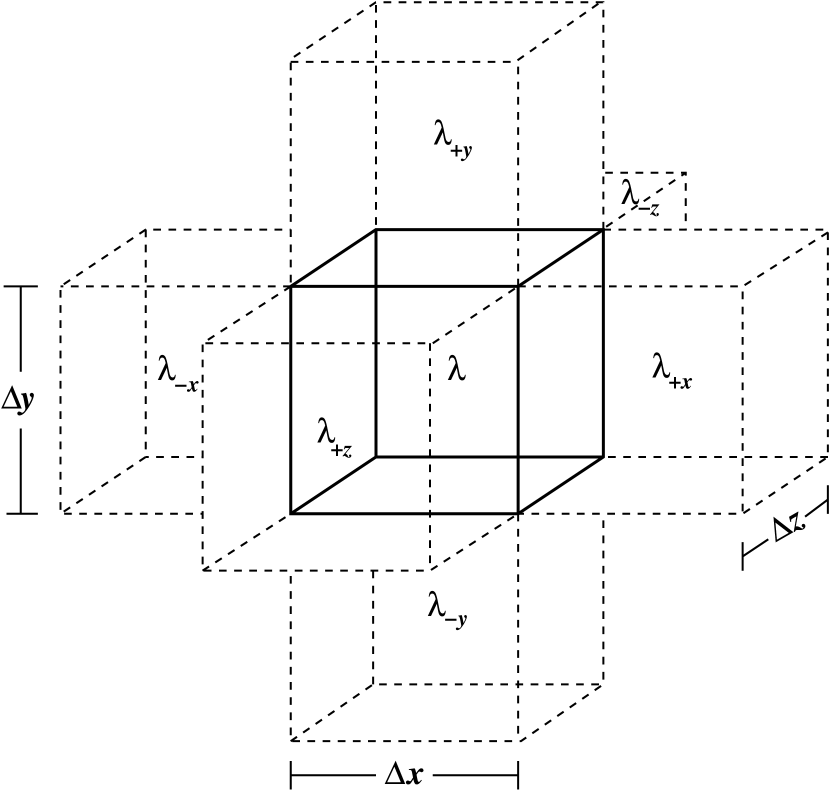
Figure 1: The geometry of a zone-centred, uniform Cartesian grid is shown. Here, $\lambda$ can be any of the five evolved quantities ($\rho$, $s$, and ${\bf J}$) or the gravitational potential ($\Phi$).

Casting the hydrodynamic equations in a sourced advective form allows the explicit conservation of mass, entropy, and momentum (insofar as the source terms allow).

3.1 Advection

The advection steps in equations (1–3) may be integrated to yield finite-difference equations for a given cell

$$\Delta\lambda=\frac{\Delta t}{\Delta V}\sum_{i=x,y,z}\left(\Lambda_{-i}-\Lambda_{+i}\right)\Delta S_{i}\,,$$ (6)

where $\Delta\lambda$ is the change in the quantity $\lambda$ due to fluid advection, $\Delta t$ is the time step, $\Delta V$ is the cell volume, $\Lambda_{\pm i}$ are the fluxes of the quantity $\lambda$ at the $\pm i$th boundary of the cell, and $\Delta S_{i}$ is the area of the cell surface normal to the $i$th direction.

In general some interpolation is required to determine the values of the fluxes at the boundaries of the cell. We break the interpolation of the fluxes into an interpolation over the fluid velocity and an interpolation over the advected quantities,

$$\Lambda_{\pm i}=\lambda^{*}_{\pm i}\overline{v}_{\pm i}\,,$$ (7)

where $\overline{v}_{\pm i}$ is the interpolated component of the velocity normal to the $\pm i$th cell face at the cell boundary, and $\lambda^{*}$ is the interpolated value of the advected quantity. The $\overline{v}_{\pm i}$ are defined by

$$\overline{v}_{\pm i}=\frac{1}{2}(v^{i}+v^{i}_{\pm i})\,,$$ (8)

where $v^{i}$ and $v^{i}_{\pm i}$ are the values of the fluid velocity in the $i$th direction at the centre of the current cell, and the centres of the neighbouring cells in the $\pm i$th directions, respectively.

A numerical difficulty with the interpolation of the advected quantities is that advecting the volumetric densities tends to generate unphysically high velocities in low cells with low mass density. We circumvent this problem by using consistent transport (Stone & Norman, 1992), in which it is the specific quantities that are interpolated, i.e.

$$\lambda^{*}_{\pm i}=\overline{\rho}_{\pm i}(\overline{\lambda/\rho})_{\pm i}\,,$$ (9)

where $\overline{\rho}_{\pm i}$ and $(\overline{\lambda/\rho})_{\pm i}$ are the interpolated values of $\rho$ and the specific quantity $\lambda/\rho$ at the $\pm i$th boundary of the cell.

The choice of the method used for interpolating the advected quantities has to be made carefully, so as to avoid introducing instabilities in the finite-difference scheme. Several such methods exist, of which we have chosen to use upwinding methods. These methods provide stability by clipping new local extrema, and limit diffusivity by interpolating quantities to the boundary in a way that accounts for the difference between the velocities associated with the upwind and downwind characteristics. Upwinding methods of various orders exist, with the the higher-order methods being necessarily more computationally expensive. The three methods we have implemented are the donor cell (zeroth-order), van Leer (first-order), and piecewise parabolic advection (PPA; second-order) methods.

3.1.1 Donor Cell Upwinding

The donor cell method is a zeroth-order upwinding scheme, approximating the spatial distribution of a given quantity, $q$, as a step function. In this method, all information from the downwind cell is ignored, i.e. at the $-i$th cell boundary

$$\overline{q}_{-i}=\left\{\begin{aligned} &q_{-i}&{\rm if}\quad\overline{v}_{-i}\geq 0\\ &q&{\rm if}\quad\overline{v}_{-i}<0\end{aligned}\right.\,.$$ (10)

For a given cell, this only requires information from the nearest neighbours. In practise, donor cell upwinding is highly diffusive (see, e.g., §5.1), and hence was not used beyond the testing stage.

3.1.2 van Leer Upwinding

The van Leer upwinding method is a first-order method first described by its namesake (van Leer, 1977a, b, 1979). In contrast to the donor cell method, the distribution of $q$ is approximated by a piecewise linear function. The slopes of these linear functions are given by the so-called van Leer slopes, defined below for a given cell along the $i$th direction,

$$dq^{i}=\left\{\begin{aligned} &\frac{2(q_{+i}-q)(q-q_{-i})}{\Delta x^{i}(q_{+i}-q_{-i})}&{\rm if}\quad(q_{+i}-q)(q-q_{-i})>0\\ &0&{\rm otherwise}\end{aligned}\right.\,.$$ (11)

In terms of the van Leer slopes, the upwinded value of the quantity $q$ at the $-i$th cell boundary is given by

$$\overline{q}_{-i}=\left\{\begin{aligned} &q_{-i}+\frac{1}{2}\left(\Delta x^{i}-\overline{v}_{-i}\Delta t\right)dq^{i}_{-i}&{\rm if}\quad\overline{v}_{-i}\geq 0\\ &q-\frac{1}{2}\left(\Delta x^{i}+\overline{v}_{-i}\Delta t\right)dq^{i}&{\rm if}\quad\overline{v}_{-i}<0\end{aligned}\right.\,,$$ (12)

where the notation $dq^{i}_{\pm j}$ denotes the van Leer slope in the $i$th direction for the neighbouring cell in the $\pm j$th direction. The van Leer method prevents the introduction of new local extrema, and hence ensures stability in the advection scheme. When the van Leer slopes vanish, the scheme reduces to the donor cell method. Note that, because van Leer upwinding uses the van Leer slopes of neighbouring cells, it requires information from both the nearest and next-nearest neighbours.

3.1.3 PPA Upwinding

The PPA method is a second-order upwinding method originally developed by Colella & Woodward (1984). It approximates the distribution of $q$ by a piecewise parabolic function. The essence of the method is the determination of the monotonized left and right interface values, $q_{L}$ and $q_{R}$, which are computed via equations (1.6)–(1.10) in Colella & Woodward (1984). In terms of $q_{L}$ and $q_{R}$, the upwinded value of $q$ at the $-i$th cell boundary is given by

$$\overline{q}_{-i}=\left\{\begin{aligned} &\begin{aligned} &q_{R,-i}+\xi(q_{-i}-q_{R,-i})\\ &\ +\xi(1-\xi)(2q_{-i}-q_{R,-i}-q_{L,-i})\end{aligned}&{\rm if}\quad\overline{v}_{-i}\geq 0\\ &\begin{aligned} &q_{L}+\xi(q-q_{L})\\ &\ +\xi(1-\xi)(2q-q_{R}-q_{L})\end{aligned}&{\rm if}\quad\overline{v}_{-i}<0\end{aligned}\right.\,,$$ (13)

where $\xi=\overline{v}_{-i}\Delta t/\Delta x^{i}$. This requires information from the nearest three neighbours.

The PPA method is substantially less diffusive than the van Leer method. This is especially notable at discontinuities, where the profiles generated by PPA are significantly steeper than those generated by the van Leer scheme. However, the improvement comes with a relatively high computational cost. It has been found by Stone & Norman (1992) that, typically, increasing the grid resolution is a computationally more efficient way to obtain greater accuracy. For this reason, unless explicitly stated otherwise, we use the van Leer upwinding method.

3.2 Artificial Viscosity

In Eulerian upwinding schemes, shocks can lead to numerical instabilities. If resolving shocks is critical, the instabilities may be cured via the introduction of Riemann solvers (capable of localising a shock to a single cell boundary). However, if resolving shocks is unnecessary, it is significantly easier to introduce an artificial numerical viscosity to smooth them out. Several prescriptions for implementing numerical viscosity can be found in the literature; we chose to implement the von Neumann-Richtmyer scheme because of its ability to produce the correct shock propagation velocity and its low dissipation far from shocks (a direct result of the fact that it acts only in regions of compression; Stone & Norman, 1992). This scheme takes the form of defining a viscous pseudo-pressure for each direction which is non-vanishing in regions of compression only:

$$Q^{i}=\left\{\begin{aligned} &l^{2}\rho\left(\frac{\partial v^{i}}{\partial x^{i}}\right)^{2}&{\rm if}\quad\frac{\partial v^{i}}{\partial x^{i}}<0\\ &0&{\rm otherwise}\end{aligned}\right.\,,$$ (14)

for $i=x,\,y,\,z$, where $l$ is the length scale over which shocks are to be smoothed. The associated source term for equation (3) is given by

$$F^{i}_{\rm visc}=-\frac{\partial Q^{i}}{\partial x^{i}}\,.$$ (15)

Typically this will smooth a shock front over a number of cells–a distance that is usually much larger than the natural shock depth. It should also be noted that a strictly correct treatment of shocks is precluded by the adiabatic condition, equation (2). This can be remedied by the inclusion of a viscous source term in the entropy equation. However, since for the applications we envision shocks will result in the rapid thermalisation of the kinetic energy of the stellar oscillations, their mere production may make a purely hydrodynamic description inapplicable. In particular, thermonuclear processes could dominate at such a point, and thus neither the added complexity and computational overhead of the Reimann solver methods nor the complication of an entropy source term are required.

3.3 Momentum Source Terms

In addition to advection, the momentum density evolves due to pressure gradients, self-gravity, and external forces (if any). We have found that simply finite-differencing $\mn@boldsymbol{\nabla}P$ leads to a less stable system than calculating the gradient via partial derivatives of the equation of state, and finite-differencing in $\rho$ and $s$. In contrast, the gravitational acceleration is obtained directly in terms of a second-order, finite-difference of the gravitational potential (the details of solving for which are presented in §4). The finite differencing of the viscous force is performed in two steps: (i) determining the viscous pseudo-pressure, and (ii) finite differencing the viscous pseudo-pressure to obtain the viscous force directly. In finite difference form, the viscous pseudo-pressure is defined by

$$Q^{i}_{\pm i}=\left\{\begin{aligned} &\eta\frac{\rho_{\pm i}+\rho}{2}\left(\frac{v^{i}_{\pm i}-v^{i}}{\Delta x^{i}}\right)^{2}&{\rm if}\quad\pm\left(v^{i}_{\pm i}-v^{i}\right)<0\\ &0&{\rm otherwise}\end{aligned}\right.\,,$$ (16)

for $i=x,\,y,\,z$. The dimensionless coefficient $\eta$ is approximately the number of cells over which discontinuities are to be smoothed. Typically, we find $\eta=2$ to be adequate. The viscous force is then determined by

$$F^{i}_{\rm visc}=-\frac{Q^{i}_{+i}-Q^{i}_{-i}}{\Delta x^{i}}\,.$$ (17)

Therefore, excluding external forces, the source terms in equation (3) are given by

$$-\left(\frac{\partial P}{\partial\rho}\right)_{s}\frac{\rho_{+i}-\rho_{-i}}{2\Delta x^{i}}-\left(\frac{\partial P}{\partial s}\right)_{\rho}\frac{s_{+i}-s_{-i}}{2\Delta x^{i}}\\ -\rho\frac{\Phi_{+i}-\Phi_{-i}}{2\Delta x^{i}}+F^{i}_{\rm visc}\,,$$ (18)

for $i=x,\,y,\,z$.

When using a barotropic equation of state, $P(\rho)$, it can be convenient to write the source terms in terms of the specific enthalpy, $h$,

$$-\rho\left(\frac{h_{+i}-h_{-i}}{2\Delta x^{i}}+\frac{\Phi_{+i}-\Phi_{-i}}{2\Delta x^{i}}\right)+F^{i}_{\rm visc}\,,$$ (19)

for $i=x,\,y,\,z$. An example of when this is useful will be discussed in §6. Note that in this case, the entropy equation is superfluous.

3.4 Courant-Friedrichs-Lewy Time Step

The stability of our explicit finite-difference scheme requires that the time step should satisfy the Courant-Friedrichs-Lewy (CFL) criterion. This corresponds to the physical consideration that, in a single time step, information should only propagate into a given cell from the neighbouring cells which are used to compute spatial derivatives at that point. A time step that is too large would require information from more distant cells, which is not available in the differencing scheme. Therefore, for stability,

$$\Delta t\leq t_{\rm CFL}\,,$$ (20)

where the CFL time is defined by

$$t_{\rm CFL}=\min\left(\frac{\Delta x}{c_{s}+|v^{x}|},\,\frac{\Delta y}{c_{s}+|v^{y}|},\,\frac{\Delta z}{c_{s}+|v^{z}|}\right)\,,$$ (21)

where $c_{s}$ is the local adiabatic sound speed (see e.g. Motl et al., 2002; Stone & Norman, 1992, and references therein). In addition, the inclusion of an artificial viscosity imposes the additional requirement that the time step does not exceed the timescale for diffusion across cell width length-scales:

$$t_{\rm visc}=\min\left(\frac{\Delta x}{4\eta|\Delta v^{x}|},\frac{\Delta y}{4\eta|\Delta v^{y}|},\frac{\Delta z}{4\eta|\Delta v^{z}|}\right)\,,$$ (22)

(see e.g. Stone & Norman, 1992). In practise, for many operator split methods, taking the time step to be the CFL time does not ensure stability. Rather, it is necessary to take $\Delta t$ to be some fraction of $t_{\rm CFL}$ or $t_{\rm visc}$. In practise, we find that a robust choice is

$$\Delta t\leq\frac{1}{4}\min\left(t_{\rm CFL},t_{\rm visc}\right)\,.$$ (23)

From equation (21) it is clear that the cells with the highest velocities (both kinetic and sound) will provide the most stringent limits on the time step. An example is the case of cells constituting the vacuum surrounding a star. In practise, for numerical reasons, no portion of the grid can have vanishing mass density. Therefore, we take ‘zero’ density to be some small fraction (typically, $10^{-8}$) of the initial maximum density. As a result, the vacuum is physically insignificant. Nonetheless, because of their large accretion velocities (though negligible momentum densities), the vacuum cells can be the limiting factor in determining the time step. To avoid this problem, we impose a velocity cap, so that the CFL time is set by only considering cells with densities larger than, say, $10^{-6}$ of the maximum density. The remaining cells have their velocities capped at

$$v_{\rm cap}=\min\left(\frac{\Delta x}{\Delta t},\,\frac{\Delta y}{\Delta t},\,\frac{\Delta z}{\Delta t}\right)\,,$$ (24)

so as to not drive the time step down. While this explicitly violates the hydrodynamic equations presented in §2, it does so in a physically negligible manner.

We use operator splitting to separate the source and advection contributions to the evolution of the fluid quantities at each time step. However, we do not use directional splitting, making our scheme a variation of the unsplit method of van Leer. Thus, a single time step is taken in three stages: (1) taking half of the source step, (2) performing the updates due to advection, and (3) taking the second half of the source step. The gravitational potential is calculated at each source sub-step.

3.5 Boundary Conditions

Because the upwinding methods require information about neighbouring cells, it is necessary to provide a boundary of ghost cells along the outer edges of the grid. As these ghost cells are not evolved themselves, they require some prescription for assigning the evolved quantities to them. We have implemented three types of boundary conditions: fixed, replicated, and outflow.

The first, and simplest, is the fixed boundary condition. In this prescription, the boundary cells are fixed to have ‘zero’ density, entropy density, and momentum flux. This tends to limit the velocity of the ‘zero’ density vacuum by not providing a boundary momentum flux.

The second set of boundary conditions consists of replicating the last set of cells in the grid. This provides a slightly more realistic set of boundary conditions, allowing the accretion of the ‘zero’ density vacuum to stabilise through hydrodynamic balance. However, if a physically significant portion of the flow is crossing the boundary, then this is significantly superior to the first scheme.

The third set of boundary conditions implemented are the so-called outflow boundary conditions. In this prescription, fluid is allowed to flow off the grid but not into it. In order to prevent the boundaries from physically affecting the fluid on the grid, the boundary values for density and entropy are chosen to preserve hydrostatic equilibrium in the last grid zone. Note that this does not stop the fluid from advecting off the grid through this zone. As a result, this will minimise the creation of spurious reflections at the boundaries. For a self-gravitating fluid configuration that is initially contained entirely within the grid, this provides the most realistic set of conditions.

3.6 Parallelisation

The primary purpose for the development of our code is to perform high resolution studies of the non-linear evolution of normal modes in white dwarfs. The resulting computational requirements necessitate high-performance computing. Because the sourced advection step for a given cell depends only upon cells in its immediate neighbourhood, it naturally lends itself to a straightforward parallelisation scheme. This takes the form of dividing the entire grid into a number of sub-domains, each of which are handled by a separate process. Because interprocess communication incurs substantial performance penalties, we need to choose a domain decomposition that minimises the communication required. The source of interprocess communication in each sourced advection step is the need for neighbour data around the edges of each sub-domain. Therefore, the time penalties due to interprocess communication are dictated by the surface area of each sub-domain, as well as the depth of neighbours that is necessary (one for donor cell upwinding, two for van Leer upwinding, and three for PPA upwinding). Hence, minimising the surface area of each sub-domain minimises the interprocess communication.

We have chosen to implement our code in the C++ programming language. This choice is motivated by considerations such as modularity of design, flexibility, efficiency, ease of code reuse, and extensibility. For example, using the object-oriented paradigm in the C++ language has allowed us to maintain a clean separation between interfaces and implementations (e.g., for the equation of state, Poisson equation solver, and initial conditions etc.), and features such as templates have allowed us to write generic code without sacrificing runtime performance.

Since standard C++ does not provide facilities for parallel computing, it is necessary to use additional libraries to handle the parallelisation. We have chosen to implement parallelisation via the Message Passing Interface (MPI). Since both optimising, ISO-compliant C++ compilers and high quality MPI implementations are available for virtually every major computing platform, our code is highly portable.

4 Solving the Poisson Equation

Equation (5) is distinct from equations (1-3) in that it requires global, rather than local, information. There are a number of methods that can be used to solve the Poisson equation. These include general elliptic equation set solvers, multigrid methods, multipole methods, and spectral methods (see e.g. Motl et al., 2002; Fryxell et al., 2000; Muller & Steinmetz, 1995; Stone & Norman, 1992). Spectral methods tend to be the most efficient, and implementing them on a regular Cartesian grid is straightforward.

The solution of the Poisson equation requires the specification of a boundary condition on some closed surface. In most physical problems, this surface is chosen to lie at infinity, upon which the potential is chosen to vanish. However, since our computational domain is finite, it is not possible to impose a boundary condition at infinity in a straightforward manner. Instead, we define the value of the potential on the surface of our domain, which we compute via a multipole expansion:

$$\Phi^{B}({\bf x})=-\sum_{l=0}^{\infty}\sum_{m=-l}^{l}\frac{4\pi G}{2l+1}r^{-l-1}Q_{lm}Y_{lm}({\bf\hat{x}})\,,$$ (25)

where

$$Q_{lm}=\int d{\bf x}^{\prime}r^{\prime l}Y_{lm}^{*}({\bf\hat{x}}^{\prime})\rho({\bf x}^{\prime})\,.$$ (26)

In practise, it is only necessary to include the first few multipoles (for our purposes $l_{\rm max}=5$) to obtain accurate boundary values. Note that the boundary condition at infinity is built into the multipole expansion.

Given the Dirichlet boundary condition, it is possible to solve Poisson equation via a discrete sine transform (DST) (see e.g. Press et al., 1992). Written in its finite-difference form, (5) becomes

$$\sum_{i=x,y,z}\frac{\Phi_{+i}-2\Phi+\Phi_{-i}}{(\Delta x^{i})^{2}}=4\pi G\rho\,.$$ (27)

In terms of their discrete sine transforms $\widehat{\Phi}$ and $\widehat{\rho}$, $\Phi$ and $\rho$ are given by

$$\Phi_{i,j,k} =\frac{2}{IJK}\sum_{m=1}^{I-1}\sum_{n=1}^{J-1}\sum_{p=1}^{K-1}\widehat{\Phi}_{m,n,p}\sin\frac{\pi im}{I}\sin\frac{\pi jn}{J}\sin\frac{\pi kp}{K}$$ (28)

$$\rho_{i,j,k} =\frac{2}{IJK}\sum_{m=1}^{I-1}\sum_{n=1}^{J-1}\sum_{p=1}^{K-1}\widehat{\rho}_{m,n,p}\sin\frac{\pi im}{I}\sin\frac{\pi jn}{J}\sin\frac{\pi kp}{K}\,,$$ (29)

where $i$, $j$, $k$, and $I$, $J$, $K$ define the location in, and the dimensions of, the computational domain, respectively. Substituting these expansions into (27) gives

$$\widehat{\Phi}_{m,n,p}=-4\pi G\frac{\widehat{\rho}_{m,n,p}}{\kappa^{2}_{m,n,p}}\,,$$ (30)

where

$$\kappa^{2}_{m,n,p} =\frac{2}{(\Delta x)^{2}}\left(1-\cos\frac{\pi m}{I}\right)$$

$$+\frac{2}{(\Delta y)^{2}}\left(1-\cos\frac{\pi n}{J}\right)$$

$$+\frac{2}{(\Delta z)^{2}}\left(1-\cos\frac{\pi p}{K}\right)\,.$$

The potential $\Phi_{i,j,k}$ is then computed from (28).

Expanding $\Phi$ in terms of the sine basis functions of the Fourier series ensures that it vanishes at the boundaries of the domain. Non-zero boundary conditions can be incorporated by adding an appropriate source term to the right side of equation (27). We may define $\Phi^{\prime}=\Phi-\Phi^{B}$ where now $\Phi^{B}$ is determined by equation (25) at one zone beyond the boundary and vanishes everywhere else. The resulting equation for $\Phi^{\prime}$ is the same as equation (27) in the interior and is given by

$$\sum_{i=x,y,z}\frac{\Phi^{\prime}_{+i}-2\Phi^{\prime}+\Phi^{\prime}_{-i}}{(\Delta x^{i})^{2}}=4\pi G\rho-\frac{\Phi^{B}_{\pm j}}{(\Delta x^{j})^{2}}=4\pi G\rho^{\prime}\,,$$ (31)

on the $\pm j$th boundary. As a result, the effective source terms are given by

$$4\pi G\rho^{\prime}_{i,j,k} =4\pi G\rho_{i,j,k}$$ (32)

$$-\frac{1}{(\Delta x)^{2}}\left(\delta_{i,1}\Phi^{B}_{0,j,k}+\delta_{i,I-1}\Phi^{B}_{I,j,k}\right)$$

$$-\frac{1}{(\Delta y)^{2}}\left(\delta_{j,1}\Phi^{B}_{i,0,k}+\delta_{j,J-1}\Phi^{B}_{i,J,k}\right)$$

$$-\frac{1}{(\Delta z)^{2}}\left(\delta_{k,1}\Phi^{B}_{i,j,0}+\delta_{k,K-1}\Phi^{B}_{i,j,K}\right)\,.$$

To summarise, our procedure for solving the Poisson equation is:

1. Calculate $\Phi^{B}$ via the multipole expansion (25).

2. Calculate the effective source terms for $\Phi^{\prime}$ from (32).

3. Perform a DST on the effective source terms.

4. Calculate $\widehat{\Phi}^{\prime}$ from (30).

5. Perform a DST on $\widehat{\Phi}^{\prime}$ to determine $\Phi^{\prime}$.

We do not actually need to add $\Phi^{B}$ to our final answer since it only affects the ghost points outside our grid. Note that, because we use a second-order finite-difference to determine the gravitational acceleration in equation (18), it is necessary to define $\Phi$ on an extra surface of ghost cells on each edge of the domain.

The DST is most efficiently parallelised in terms of a slab decomposition of the grid, as opposed to the ideal decomposition for the sourced advection step (which is cubical). As a result, a significant amount of interprocess communication is required to prepare for the solution of the Poisson equation at each source sub-step. However, we have found that the time saved by using the DST more than outweighs the penalty incurred by the communication overhead compared to alternative methods.

5 Test Problems

5.1 Advection

Figure 2: A square pulse that has been advected five times its initial width (50 cells) using the donor cell (open circles), van Leer (filled triangles), and PPA (open squares) upwinding schemes. For reference, the original pulse profile is also shown.

In order to test the advection scheme, we considered the advection of a square pulse (without source terms). In Figure 2, the pulse is shown after being advected five times its initial width (50 cells) using both the donor cell and van Leer upwinding methods. It is clear that both methods are diffusive, with the donor cell method substantially more so.

Figure 3: A sine wave is advected with periodic boundary conditions for 100 times its wavelength (200 cells) using the van Leer (filled triangles) and PPA (open squares) upwinding schemes. In the top panel the density profile is shown explicitly, while in the bottom the residuals are plotted. For reference the analytical result is also shown.

In general, diffusion will lead to errors in both the amplitude and the phase of an advected pulse. In order to quantify these errors for diffusion resulting from the upwinding scheme, a sine wave was advected with periodic boundary conditions for 100 times its wavelength. By this time, the donor cell upwinding scheme has diffused the sine wave completely, hence only the van Leer and PPA methods are shown in Figure 3. The errors are at the 4% and 0.4% levels, respectively, with deviations becoming most significant at extrema. In both the square pulse and the sine wave, a noticeable asymmetry (which is determined by the direction of propagation) develops as a result of higher-order effects in the upwinding schemes.

5.2 Sod Shock Tube

The pressure source term in equation (3) was tested by the Sod shock tube problem. The Sod shock tube consists of an initial density and pressure discontinuity, and its subsequent evolution for an ideal gas ($\Gamma=1.4$) and a specific set of initial conditions. For $x>0$, $\rho=0.125$ and $P=0.1$, while for $x\leq 0$, $\rho=1$ and $P=1$. Because it is the entropy density and not the pressure that is evolved, it is necessary to find $s$ as a function of $\rho$ and $P$ for an ideal gas:

$$s=\ln\left(\frac{P^{n}}{\rho^{n+1}}\right)\quad{\rm where}\quad n=\frac{1}{\Gamma-1}\,.$$ (33)

The Sod shock tube is useful as a test because the resulting $\rho$ and $P$ profiles for any given time can be calculated analytically (see, e.g., Sod, 1978; Hawley et al., 1984).

Figure 4: The density, pressure, velocity, and entropy are shown for the Sod shock tube at $t=0.2$ (the units of which depend upon the units chosen for the pressure and density). 200 cells were used with van Leer upwinding. The head and tail of the rarefaction wave are located at $x=-0.235$ and $x=-0.014$, respectively. The contact and shock discontinuities are at $x=0.184$ and $x=0.35$, respectively.

In Figure 4, the numerical results from our code are compared to the analytical solutions. Overall, they are in good agreement, with the exception of two minor discrepancies. The most notable discrepancy is the entropy deficit in the post-shock fluid ($0.184<x<0.35$). This is a result of using the adiabatic condition, and thus ignoring entropy production at shocks. Hence, the higher analytical value is easy to understand. Because we intend to apply the code to scenarios in which the adiabatic condition holds to a very good approximation, we expect the entropy deficit to be physically insignificant. The second discrepancy is the overshoots at points where the slopes of quantities change discontinuously. As discussed in Stone & Norman (1992), this is a real result, originating from the numerical viscosity inherent in any finite-difference code. The most important result, however, is the fact that the artificial viscosity causes the shock fronts to be well behaved in our code.

5.3 Pressure-Free Collapse

The gravitational source term in equation (3) was tested via the pressure-free collapse of a uniform density sphere. Once again, there is an analytical solution:

$$r =r_{0}\cos^{2}\beta$$

$$\rho =\rho_{0}\cos^{-6}\beta$$ (34)

$$t =\left(\beta+\frac{1}{2}\sin 2\beta\right)\left(\frac{8\pi}{3}G\rho_{0}\right)^{-1/2}\,,$$

(see, e.g., Stone & Norman, 1992). Figure 5 depicts the result after allowing the radius to halve (at $t=0.909$ for $G=1$), for a $256\times 256\times 256$ cell grid. There is a small excess on the edges resulting from our implementations of viscosity and consistent transport (which necessarily treats the advection of velocity into the edges differently due to the density gradients). Overall, it does show good agreement with the analytical prediction.

Figure 5: The numerical (open circles) and analytical (solid line) solutions for the density as a function of distance along a radial section for the pressure free collapse of a uniform density sphere are shown. The initial radius and total mass of the sphere was unity. A $256\times 256\times 256$ cell grid was used. With Newton’s constant given by $G=1$, this occurs at $t=0.909$.

6 Application to a Pulsating White Dwarf

6.1 Hydrostatic Equilibrium

The problem of choosing an equilibrium fluid configuration is made non-trivial by the finite differencing of the the dynamical equations. Consequently, a method to produce an equilibrium solution for the finite difference equations is required. For a barotropic equation of state, we have chosen to make use of the self-consistent field (SCF) method (see, e.g., Motl et al., 2002; Hachisu, 1986; Ostriker & Mark, 1968). Because it is well described elsewhere, we will only summarise the procedure here.

1. An initial guess for the density (taken from the continuous solution) is used to generate the gravitational potential via the method described in §4.

2. The new gravitational potential and the initial density guess are then used to calculate the Bernoulli constant at the centre of the star.

3. the Bernoulli constant and the new gravitational potential are used to calculate the enthalpy at all points on the grid, which is then subsequently inverted to yield the new density guess.

This procedure is iterated until the Bernoulli constant converges to some specified tolerance–i.e. when the fractional change is less than some small value (say, $10^{-12}$). The resulting density distribution is a solution to

$$\frac{h_{+i}-h_{-i}}{2\Delta x^{i}}+\frac{\Phi_{+i}-\Phi_{-i}}{2\Delta x^{i}}=0\,,$$ (35)

and, hence, no net momentum flux is generated if the source terms are given by equation (19). Note that, if the source terms are given by equation (18), this may still produce a net momentum flux, and is not necessarily a good approximation to equilibrium in that case.

Model	$M\,(M_{\odot})$	$R\,(10^{6}{\rm m})$	$\omega_{*}\,({\rm Hz})$	$\omega_{f2}\,({\rm Hz})$	$\omega_{p2}\,({\rm Hz})$
CWD	0.632	8.56	0.365	0.562	1.15
HWD	0.632	11.2	0.243	0.560	0.749

Table 1: Stellar properties for a cold white dwarf with (CWD) and without (HWD) an isothermal envelope. Specifically, the mass, radius, fiducial stellar frequency $\omega_{*}=\sqrt{GM/R^{3}}$, frequency of the adiabatic quadrupolar fundamental mode, and the frequency of the lowest order adiabatic quadrupolar $p$-mode. Note that the inclusion of the isothermal envelope does not change the mass appreciably while significantly increasing the radius.

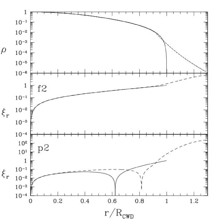
Figure 6: Shown in the top panel are the density profiles for the cold white dwarf with (solid) and without (dashed) the isothermal envelope. The two lower panels are the radial displacement profiles for the quadrupolar fundamental mode ($f2$) and the lowest order quadrupolar $p$-mode ($p2$) for the two models. Note that the density and $f2$ mode profiles are very nearly the same for the two cases. However, the mode profiles differ substantially for the $p2$ mode.

When

$$\left|\frac{\partial P}{\partial x^{i}}\right|>\frac{P}{\Delta x^{i}}\,,$$ (36)

the pressure gradient required to preserve hydrostatic equilibrium cannot be resolved on the grid. For a star, this can result in strong, inwardly directed forces at the surface, driving shocks into the interior. We have found that adding an isothermal envelope can mitigate this problem by pushing the region where this inequality is true off the grid, while adding an insignificant amount of mass to the star itself. This is done explicitly by setting a fiducial density (which we chose to be $10^{-2}$ of the central density) at which the equation of state changes from that of a cold white dwarf to a $\Gamma=1$ polytrope. The polytropic constant is chosen such that $P(\rho)$ remains continuous across the transition. Table 1 compares the properties of the cold white dwarf with (HWD) and without (CWD) the isothermal envelope. Note that while the isothermal envelope increases the radius significantly, it does not change the mass or the frequency of the quadrupolar fundamental mode ($\omega_{f2}$). The reason for this can be seen in Figure 6. The $f2$ mode is more strongly weighted in the core where the addition of the isothermal envelope makes no difference. In contrast, the lowest-order quadrupolar $p$-mode is substantially affected by the presence of the envelope. This probably results from the fact that the radial wavelength of the $p2$ is much closer to the height of the isothermal envelope. Henceforth, all evolutions were begun with the HWD model listed in Table 1.

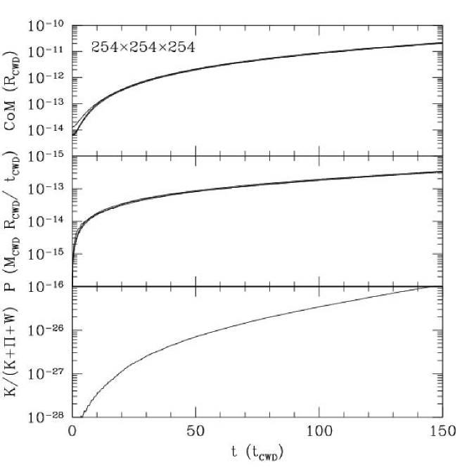
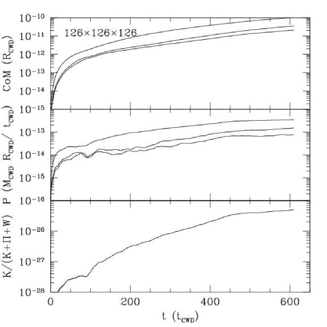
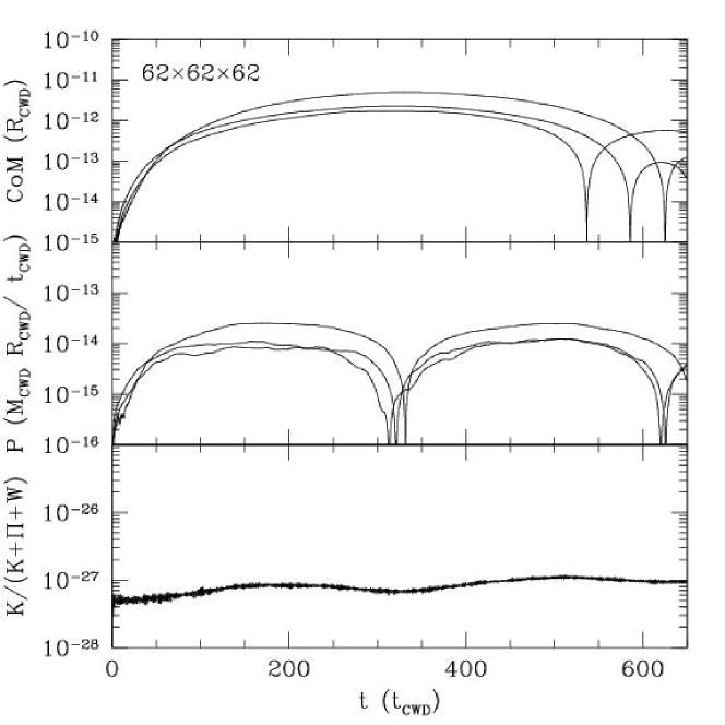
Figure 7: Shown are the centre-of-mass (top panels), net momentum (middle panels), and fraction of the total energy converted into kinetic energy (bottom panels) for a number of grid resolutions (note the different time scales). In all cases these quantities saturate well below significant levels (e.g., for the worst case, the centre-of-mass moves by less than $10^{-8}$ cell widths in the 150 dynamical times shown, thus it would require roughly $10^{13}$ dynamical times before the centre-of-mass moves one stellar radius. Typically, these appear to turn over, implying that they may never rise significantly above $10^{-7}$ cell widths.)

The quality of the equilibrium generated by the SCF method may be explicitly demonstrated. Figure 7 shows the evolution of the centre-of-mass position, net momentum, and the fraction of the total energy that is converted into kinetic energy for a star initially in hydrostatic equilibrium. The last quantity is given in terms of the kinetic, internal, and gravitational components:

$$K=\int\frac{1}{2}\rho v^{2}\,d^{3}x\,,\quad\Pi=\int p\,d^{3}x\,,\quad W=\int\rho\Psi\,d^{3}x\,.$$ (37)

Despite an initial exponential rise, these quantities saturate at relatively low levels for all resolutions shown. Note that all times are measured in dynamical times of the cold white dwarf, $t_{\rm CWD}\equiv 1/\omega_{*}$, which is approximately the time it takes for a disturbance to cross the star.

6.2 Oscillation Modes

In general, the problem of interest is dynamical. Specifically, we are interested in the non-linear evolution of the oscillation modes of a cold white dwarf which are being excited resonantly by tidal forces. Towards this end, it is important to obtain a measure of the numerical quality factor ($Q$; the $e$-folding time of the energy in the oscillation), and the oscillation frequencies themselves. That the latter may be different from the frequencies in Table 1 is a result of both the approximation of discrete cells and the fact that the finite-difference equations are distinct from the continuous equations. However, we expect the deviation to be small, and therefore a close agreement between the predicted and observed frequencies serves as yet another test for the correctness of our code. Both the quality factor and the oscillation eigenfrequencies can be obtained by deforming the star in a particular way, and analysing the subsequent oscillations.

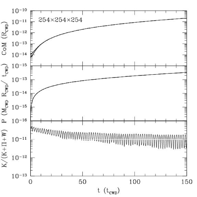
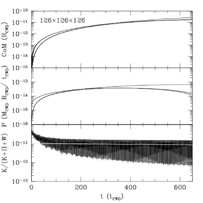
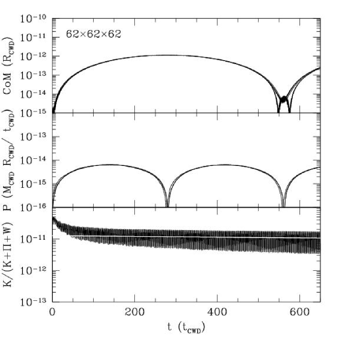
Figure 8: Same as Figure 7 for the case when a quadrupolar perturbation is present (note the difference in scales in comparison to that figure). The white line drawn through the oscillations is for a $Q$ of approximately 6000.

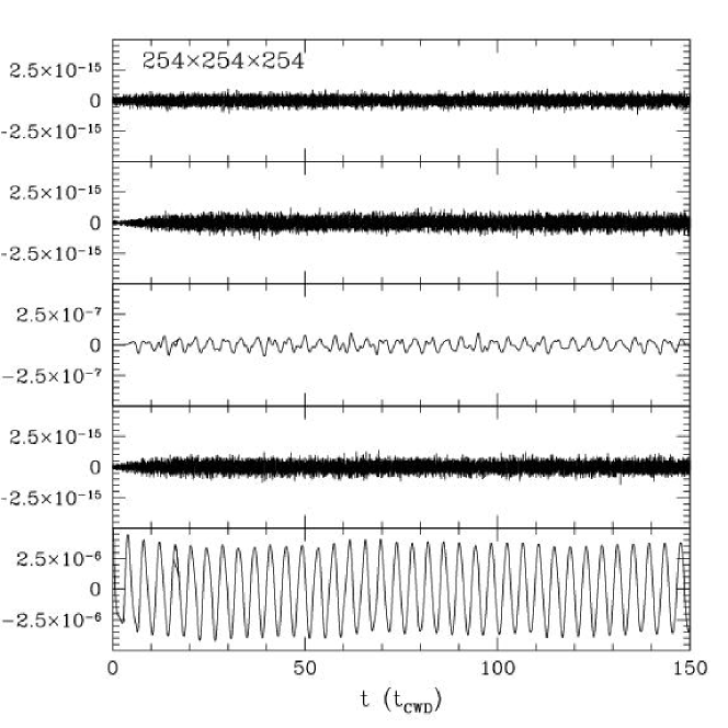
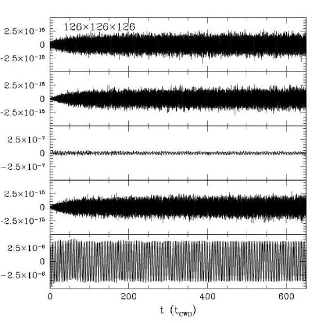
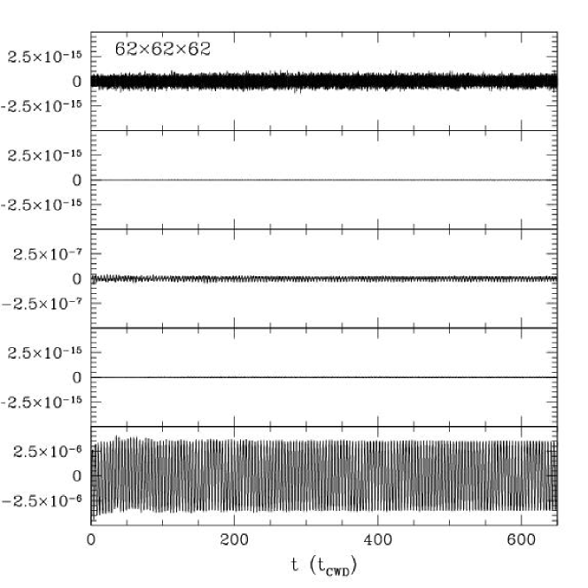
Figure 9: The quadrupolar moments of the perturbed star for each of the resolutions considered in Figure 8. From top to bottom, the panels are the odd $m=2$, odd $m=1$, $m=0$, even $m=1$, and even $m=2$ moments. Note the difference in scales of the different moments, namely that the even $m=2$ moment is two orders of magnitude larger than the $m=0$ moment (which is sourced by the Cartesian geometry) and nine orders of magnitudes larger than the others.

We deformed the star by adding a fractional quadrupolar perturbation to the density, i.e.

$$\Delta\rho({\bf r})=A\rho(r)Y^{e}_{22}(\theta,\phi)\,,$$ (38)

where the amplitude, $A$, was chosen to be small ($10^{-4}$) so that the resulting oscillation occurred in the linear regime. This initiated an even $m=2$ standing wave on the star. Figures 8 and 9 show the resulting evolutions for a number of grid resolutions. The same diagnostics as those used to demonstrate hydrostatic equilibrium are shown in Figure 7. In this case as well, the centre-of-mass and momentum drift saturate at levels well below those of interest. Unlike hydrostatic equilibrium, there now exists a non-vanishing kinetic energy. It is strongly harmonic and decays exponentially. Because the initial perturbation excited all of the even quadrupolar modes with $m=2$, there are a number of distinct decay constants, with the slowest being due to the $f2$ mode. This exponential decay at late times may be fit to estimate the numerical $Q$, found here to be on the order of $6000$.

Figure 10: Shown are the power spectra of the even $m=2$ quadrupolar moment as a function of angular frequency (using the mean squared amplitude normalisation). As expected, for each grid resolution there is a strong spike coincident with the $f2$ mode frequency predicted for the HWD model.

In Figure 9, the quadrupolar moments are shown. The even $m=2$ moment is strongly dominant as expected. It also has a very clear harmonic structure. This may be Fourier analysed to produce the dominant oscillation mode, as shown in Figure 10. In the power spectrum of the even $m=2$ quadrupolar moment, there is a peak which extends five orders of magnitude above the rest of the spectrum. This peak is clearly identifiable with the $f2$ mode, and appears to have very nearly the frequency predicted by the HWD model.

7 Conclusions

We have developed and tested a parallel, simple and fast hydrodynamics code for multi-dimensional, self-gravitating, adiabatic flows. Both the advection terms and the solution for the self-gravity are greatly simplified by the use of a uniform Cartesian geometry, ultimately leading to explicit conservation of mass, entropy, and momentum to nearly numerical accuracy. The simplifying assumption of adiabaticity and the absence of shocks eliminate the necessity for more numerically expensive schemes, yielding an efficient code.

We have also applied our code to a number of standard diagnostic problems in order to verify its physical correctness and limitations. This has been done in a systematic fashion intended to test each aspect of the code separately, including the advection scheme, the pressure source terms, and finally the gravitational potential. Finally we have demonstrated the fitness of the code for the problem which motivated its development: the study of tidally excited adiabatic oscillations on white dwarfs. This has been done in two stages: firstly, verifying the long term numerical stability of a white dwarf in hydrostatic equilibrium, and, secondly, measuring the numerical quality factor (found to be on the order of 6000) and the quadrupolar fundamental mode frequency (found to be very nearly that predicted by a linear mode analysis of the white dwarf model). The details of tidally exciting adiabatic oscillations with non-linear amplitudes on cold white dwarfs, and their subsequent evolution will be discussed in a future publication.

References

- Colbert & Ptak (2002) Colbert E. J. M., Ptak A. F., 2002, ApJS, 143, 25
- Colella & Woodward (1984) Colella P., Woodward P. R., 1984, J. Comp. Phys., 54, 174
- Fryxell et al. (2000) Fryxell B., Olson K., Ricker P., Timmes F. X., Zingale M., Lamb D. Q., MacNeice P., Rosner R., Truran J. W., Tufo H., 2000, ApJS, 131, 273
- Gerssen et al. (2002) Gerssen J., van der Marel R. P., Gebhardt K., Guhathakurta P., Peterson R. C., Pryor C., 2002, AJ, 124, 3270
- Hachisu (1986) Hachisu I., 1986, ApJS, 62, 461
- Hawley et al. (1984) Hawley J. F., Wilson J. R., Smarr L. L., 1984, ApJ, 277, 296
- Madau & Rees (2001) Madau P., Rees M. J., 2001, ApJL, 551, L27
- Motl et al. (2002) Motl P. M., Tohline J. E., Frank J., 2002, ApJS, 138, 121
- Muller & Steinmetz (1995) Muller E., Steinmetz M., 1995, Comp. Phys. Comm., 89, 45
- Ostriker & Mark (1968) Ostriker J. P., Mark J. W.-K., 1968, ApJ, 151, 1075
- Press et al. (1992) Press W. H., Teukolsky S. A., Vetterling W. T., Flannery B. P., 1992, Numerical recipes in C. The art of scientific computing. Cambridge: University Press, —c1992, 2nd ed.
- Rathore et al. (2004) Rathore Y., Blandford R. D., Broderick A. E., 2004, MNRAS
- Rathore et al. (2003) Rathore Y., Broderick A. E., Blandford R., 2003, MNRAS, 339, 25
- Sod (1978) Sod G. A., 1978, J. Comp. Phys., 27, 1
- Stone & Norman (1992) Stone J. M., Norman M. L., 1992, ApJS, 80, 753
- van Leer (1977a) van Leer B., 1977a, J. Comp. Phys., 23, 263
- van Leer (1977b) van Leer B., 1977b, J. Comp. Phys., 23, 276
- van Leer (1979) van Leer B., 1979, J. Comp. Phys., 32, 101