The influence of the geomagnetic field and of the uncertainties in the primary spectrum on the development of the muon flux in the atmosphere.

Abstract

In this paper we study the sensitivity of the flux of atmospheric muons to uncertainties in the primary cosmic ray spectrum and to the treatment of the geomagnetic field in a calculation. We use the air shower simulation program AIRES to make the calculation for two different primary spectra and under several approximations to the propagation of charged particles in the geomagnetic field. The results illustrate the importance of accurate modelling of the geomagnetic field effects. We propose a high and a low fit of the proton and helium fluxes, and calculate the muon fluxes with these different inputs. Comparison with measurements of the muon flux by the CAPRICE experiment shows a slight preference for the higher primary cosmic ray flux parametrization.

I Introduction

The study of the muon fluxes in the atmosphere is currently of great interest because of the correlation between the muon and neutrino fluxes. Atmospheric neutrinos are produced from the decay channels of pions and kaons and the subsequent muon decay. The production of electron and muon neutrinos is dominated by the processes $\pi^{+}\rightarrow\mu^{+}+\nu_{\mu}$ followed by $\mu^{+}\rightarrow e^{+}+\overline{\nu}_{\mu}+\nu_{e}$ (and their charge conjugates), with a similar chain for charged kaons. When all particles decay, there will be two muon neutrinos for each electron neutrino resulting in an expected ratio $\nu_{\mu}/\nu_{e}$ of the flux of $\nu_{\mu}+\overline{\nu}_{\mu}$ to the flux of $\nu_{e}+\overline{\nu}_{e}$ of about 2. The experimental measurements k1 ; k2 ; imb ; sk1 ; frejus ; nusex ; ultima indicate, however, that the ratio of muon to electron neutrinos in the atmosphere is significantly smaller than two.

This disagreement with theoretical predictions has been interpreted in terms of neutrino oscillations oscila . In order to calculate precisely the neutrino oscillation parameters one has to know the neutrino flux at production. Because of the close connection beteween the neutrinos and the muons, a standard test of codes used for calculating the neutrino flux is to calculate the muon flux with the same procedure and compare it to measurements of muons. Our approach here is related but somewhat different. We calculate only the muon flux, and we use the comparison with measurements to probe two aspects of the input that are common to both the neutrino and the muon fluxes.

The calculation of both muons and neutrinos starts with the primary spectrum outside the atmosphere. Therefore uncertainties in the measurements of the primary spectrum of protons, helium and heavier nuclei affect both fluxes in a similar way. Because the uncorrelated fluxes depend essentially on energy per nucleon, heavy nuclei have relatively little effect, and the largest uncertainty in normalization comes from protons and helium. Experimental measurements of primary proton and helium spectra in some cases show significant differences from each other. We find that it is possible to divide the experimental data over a fairly large energy range into two groups: group 1 corresponds to the data wich give a lower flux and group 2 to a higher flux. By making a “high” fit and a “low” fit over an extended energy range, we can define a reasonable range where the primary spectum should lie. Comparison with measured muon fluxes may provide an extra constraint on the normalization of the primary flux.

Treatment of the geomagnetic field affects both the neutrino and the muon fluxes. One effect is a consequence of the field acting on the primary cosmic rays, which determines allowed and forbidden trajectories. Primaries on allowed trajectories reach the atmosphere to interact and produce secondary muons and neutrinos while those on forbidden trajectories do not reach the atmosphere and therefore do not contribute to secondary fluxes. The other significant effect is the bending of charged muons after production in the atmosphere. Which trajectories are allowed and which forbidden depends both on magnetic rigidity (defined as total momentum divided by charge of the nucleus) and on the direction of the particle. At high geomagnetic latitudes all primaries with energies above pion production threshold are allowed. At low latitudes, particles need to have a minimum rigidity to reach the atmosphere, and this minimum value is higher for positive particles from the East than from the West. We investigate the sensitivity of the muon fluxes to both aspects of the geomagnetic field as a function energy and atmospheric depth.

The paper is organized as follows: Section II is divided in three subsections. In II.1 we report on the method used to calculate the atmospheric muon fluxes; in II.2 we describe the treatment of the geomagnetic field; and in II.3 we propose the high and low fits of the primary proton and helium spectrum data. The results are reported in III and finally we summarize our conclusions in section IV.

II The simulations

II.1 Air shower simulations

In this work we have used the Air Shower Simulation Program (AIRES) AIRES ; AIRESManual , which provides full space-time particle propagation and accounts for the atmospheric density profile atmosfera and the Earth’s curvature. The particles taken into account by AIRES in the simulation are: gammas, electrons, positrons, muons, pion, kaons, lambda baryons, nucleons, antinucleons and nuclei up to Z=36. The hadronic processes are simulated using different models, according with their energy. High energy collisions are processed invoking an external package, SIBYLL or QGSjet (SIBYLL 2.1 SIBYLL or QGSjet01 QGSJET ), while low energy ones are processed using an extension of the Hillas splitting algorithm (EHSA)AIRES ; AIRESCCICRC ; AUGERJPG . In this work we use SIBYLL. The threshold energy separating the low and high energy regimes is 200 GeV. The effect of the geomagnetic field (GF) inside the atmosphere is taken into account in AIRES. The GF calculations are controlled from the input instruction by specifying a date and the geographic coordinates of a site. The program uses the IGRF model GF to evaluate the magnetic field intensity and orientation. It is assumed that the shower develops under the influence of a constant and homogeneous field which is evaluated before starting the simulations.

The input used in the simulation and the procedure to calculate the flux is the same as that used in Ref sergioyyo . In Ref sergioyyo the CAPRICE experimental geomagnetic transmission function was used to estimate the cutoff prior to the calculation of the muon flux. Here we use a more precise backtracking method, as described in the next subsection.

II.2 Geomagnetic field effects

The magnetic field affects the low energy muon flux both through the geomagnetic cutoffs on the primary cosmic rays, including the East-West effect, and by the bending of trajectories of secondary charged particles inside the atmosphere.

The East-West effect is the suppression of cosmic ray nuclei incident on the atmosphere from the East compared to those from the West. This suppression is due to the combination of the following two facts johnson alvarez :

-

Positively charged particles at the same zenith angle have a higher cutoff from the East direction than from the West (and vice-versa for negatively charged particles) since some of their trajectories intersect the Earth.

-

Cosmic rays are positively charged nuclei, so they will bend in one sense in the geomagnetic field.

To calculate these geomagnetic effects we use backtracking technique in a detailed, time-dependent geomagnetic field model (IGRF, International Geomagnetic Field model). This technique consists of the integration of the equation of motion of a particle with the opposite charge starting at a position near the top of the atmosphere. We inject antiprotons outwards from an altitude of 100 km in various directions and see if the backtracked antiproton reaches a distance of 30 R_⊕ from the Earth within a total pathlength of 300 R_⊕. Any direction in which an antiproton of a given momentum can reach this distance is an allowed direction from which a proton of the opposite momentum can arrive. The backtracked antiprotons that do not reach that distance are either trapped in the geomagnetic field or their trajectories intersect the surface of the Earth. In these last two cases the trajectory is considered forbidden. The results are expressed in terms of a transmission function, also called penetration probability, which is zero at low rigidity and increases to one at higher rigidity. The energy dependence of the transmission function depends on the geomagnetic latitude and the angle between the cosmic ray direction and the geomagnetic field lines. The geomagnetic cutoff is treated in the simulation by the application of this function to the input primary cosmic ray flux,

To explore the East-West effect we have compared two transmission functions, one averaged over primaries inside a cone of half angle 30^∘ from the East and the other over a similar cone from the West.

The CAPRICE Geomagnetic transmission function emiliano used in Ref. sergioyyo was obtained by comparing the shape of the spectra of alpha particles measured by the balloon borne experiment CAPRICE94 boe99b with the shape of CAPRICE98 amb99 . These two balloon experiments flew in different locations: the first in Lynn Lake, Manitoba, Canada, where the geomagnetic cutoff is negligible, and the other in Ft. Summer New Mexico (USA) where the vertical cutoff is 4.3 GV. This transmission function is only a function of rigidity and therefore does not produce the East-West effect. We compare the two methods in Section III below.

II.3 The low and high fits to the primary Spectrum data

New measurements of the primary spectra of protons and helium have improved our knowledge of the primary spectrum up to 100 GeV compared to what was previously known. There are nevertheless still significant discrepancies between different experiments. For this reason we have performed two different fits: one with the experiments that give the lowest (we will call them Group 1) and another that give the highest fluxes (Group 2). All these measurements were fitted to the following function:

$$\phi(E_{k})=k\times(E_{k}+b\phantom{0}exp\left(-c\sqrt{E}_{k}\right))^{-\alpha}$$ (1)

where $E_{k}$ is the kinetic energy per nucleon hamburgcrf , and $\alpha$ and $k$ are free parameters.

Group 1 consists of the data of CAPRICE98 emiliano , Atic ATICi ATIC below 100 GeV and RunJob RunJOB RunJOBi at high energy. Group 2 consists of the data of AMS AMSp  AMSh , BESS Bess at low energy and JACEE Jacee at high energy (There was not a considerable difference between AMS-JACEE and BESS-JACEE fit for the protons fluxes).

In figure 1 we show the combination of the experimental data on the proton fluxes for the experiments of group 1 (left) and for group 2 (right). Three different fits are shown in the left-hand panel. The solid line corresponds to the fit of all the data. We have also made separate fits for the low energy data (the dashed line) and for the high energy data (the dotted line). The left hand side of the figure 1 shows the proton data from AMS with full circles, BESS with open circles and JACEE with stars. We have done two fits for the following two groups AMS-JACEE (solid line) and BESS-JACEE (dashed line).

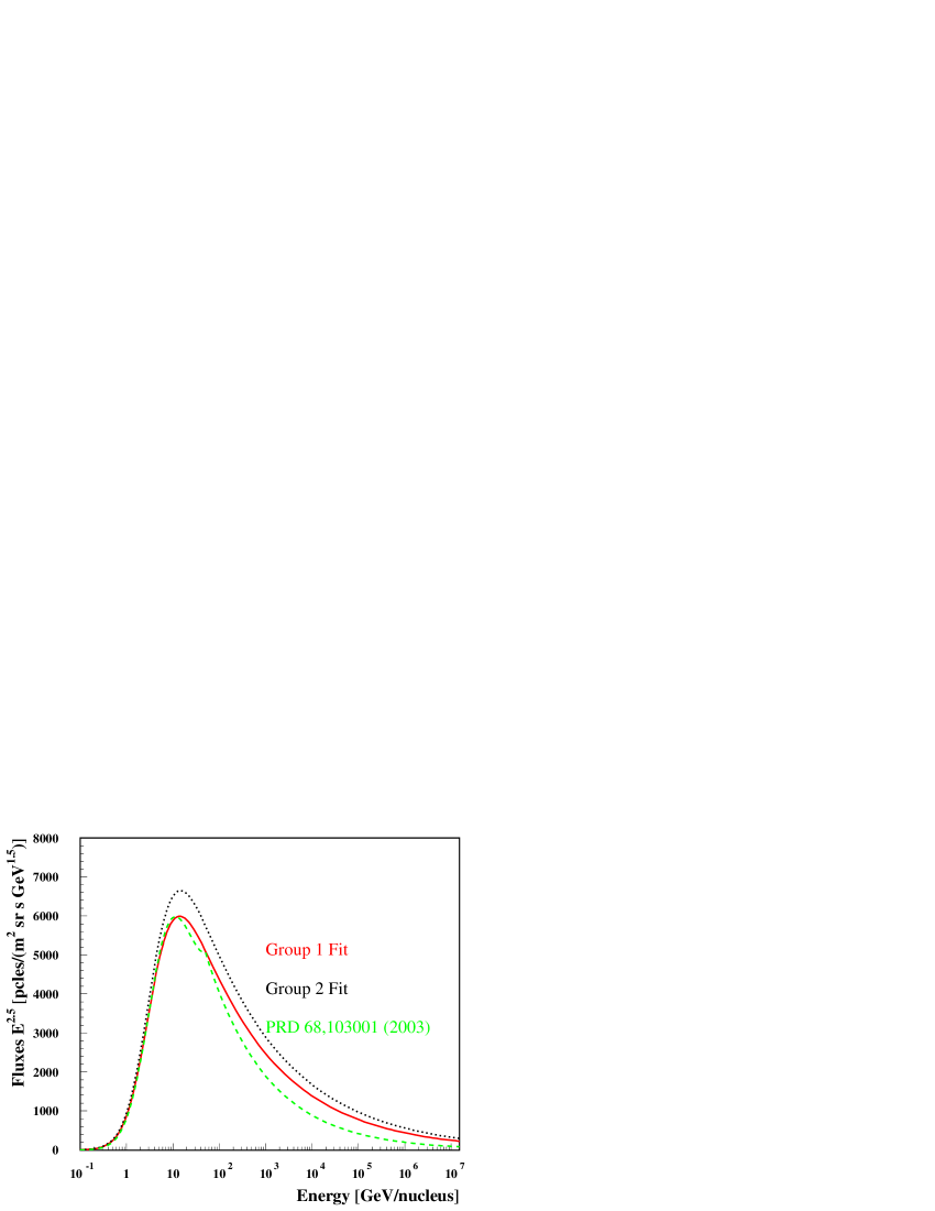
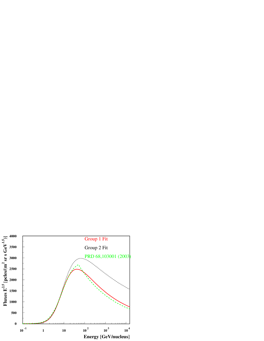
Figure 3: Fluxes of proton (left) and helium (right) at the top of the atmosphere, plotted as function of the kinetic energy of the primaries. (1) Solid line: Group 1 fit. (2) Dotted line: Group 2 fit. (3) Dashed line: Input used in Ref. sergioyyo .

Figure 2 shows the helium experimental data for group 1 (left) and group 2 (right). For group 1 we have made two fits with different values of b and c. For group 2 there is a considerable difference between the data of AMS and JACEE. This is not the case in a combination of BESS and JACEE data. For this reason we performed two different fits but implement in the calculation the BESS-JACEE data fit. The parameters for the fluxes of group 1 and group 2 are shown in table 1. To have a clear picture in figure 3 we show three different fits of the absolute fluxes of proton (left) and helium (right) that we will use in this calculation (Group 1, Group 2 and that of Ref. sergioyyo ).

Table 1: Parameters for the Hydrogen and Helium components in the fit of Equation 1 for the two data groups.

Group	Component	00000$\alpha$	0000 $k$	0$b$	0 $c$
001	Hydrogen	2.751 $\pm$ 0.004	14000 $\pm$ 130	2.15	0.21
001	Helium	2.734 $\pm$ 0.005	657 $\pm$ 8	1.25	0.14
002	Hydrogen	2.738 $\pm$ 0.004	15000 $\pm$ 160	2.15	0.21
002	Helium	2.639 $\pm$ 0.008	615 $\pm$ 16	1.25	0.14

The fluxes of H and He were complemented by fluxes of heavy nuclei in eight groups that were fitted to the available data as in Ref. sergioyyo . The extensions of the spectra of heavy nuclei are not extremely important for the calculations of the atmospheric muon fluxes because H and He nuclei provide 85 to 90% of the all nucleon fluxes. The potential error from inexact fitting of the spectra of heavy nuclei would not exceed 3% of the all nucleon flux. It is the normalization of the proton fluxes that dominate the difference in muon fluxes between group 1 and group 2.

III Results

III.1 Geomagnetic field effects.

To check the validity of the transmission functions we have calculated the flux of protons at an altitude of 5.5 g/cm² where we have experimental results from the CAPRICE98 experiment. In figure 4 the proton flux at 5.5 g/cm² is plotted on the left as a function of momentum. The full points correspond to the data of the proton flux at 5.5 g/cm² from CAPRICE98 experiment emilianot and the lines are the proton fluxes obtained by the AIRES simulation. The narrow solid line is without applying any transmission function, the wide solid line is using the CAPRICE transmission function and the dotted is applying the theoretical transmission function. We are able to reproduce quite well the proton flux at 5.5 g/cm² emilianot using both the CAPRICE and the theoretical transmission functions.

To illustrate the East-West effect we apply to our input flux the theoretical geomagnetic transmission function but selecting primaries particles that only came from the East or from the West. In figure 4 on the right the dotted line corresponds to the flux of protons calculated using the theoretical geomagnetic transmission function from the West. The wide solid line corresponds to protons from the East. There is a definite excess of protons that come from the West at energies lower than 10 GeV.

The effect of this excess on the muon fluxes is illustrated in figures 5 and 6. In these two figures we plot the muon flux coming from the West (dotted line) and coming from the East (solid line) as a function of the momentum. In the two figures it is possible to see that the excess of muons coming from the West decreases with increasing atmospheric depth and is negligible at the ground. To quantify the results we calculate the relative differences between the East West fluxes for positives and negative muons. It was found that the relative differences between the two directions for muons of energy around 0.2 GeV is of order of 25 % at 5.5 g/cm², 10 % at 219 g/cm², 5 % at 462 g/cm² and null at ground.

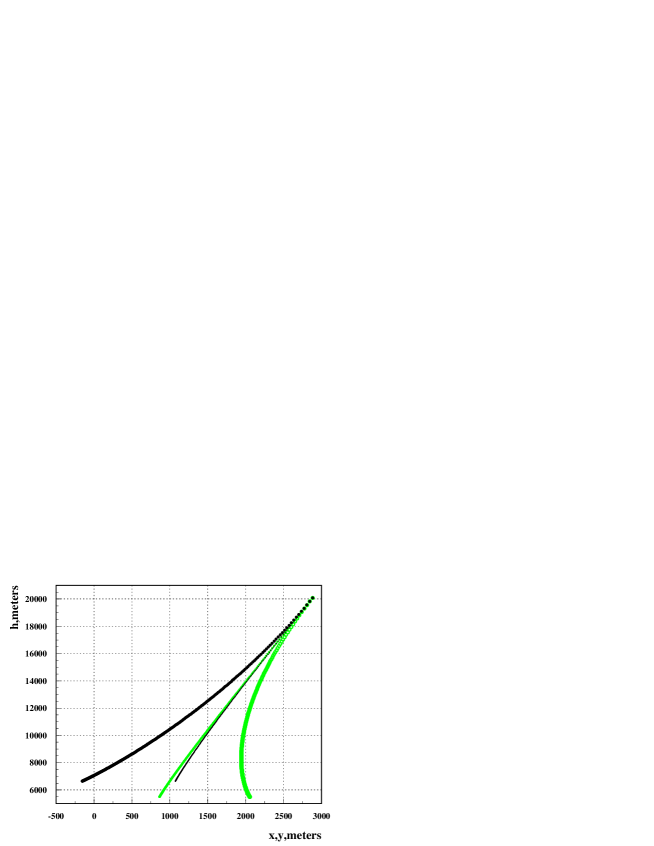
Figure 7: A positive and a negative 1 GeV/c muon injected at 20 Km with $cos(\theta)$=0.98 and azimuth=45⁰ bending in the Geomagnetic field at For Sumner in x and y direction and followed to decay. (1) Narrow light line: Negative muon deflected in $x$ direction. (2) Wide light line: Negative muon deflected in $y$ direction. (3) Narrow solid line: Positive muon deflected in $x$ direction. (4) Wide solid line: Positive muon deflected in $y$ direction. The weight of the particle curves depend on the azimuth angle and is stronger when the particle are perpendicular to $B$.

The muon flux also changes because of the bending in the local magnetic field inside the atmosphere. Figure 7 illustrates this effect by comparing two trajectories, one of a positive muon, the other of a negative muon. We injected a positive and a negative muon, each of 1 GeV, at 20 Km with zenith angle of $11^{\circ}$ and azimuth of $45^{\circ}$. The muons were followed until decay in the geomagnetic field at Fort Sumner. The narrow dark line is a negative muon deflected in x direction and the wide dark line in y direction. The narrow light line is a positive muon deflected in x direction and the wide line a positive deflected in y direction. It is possible to see that the positive muon decays before reaching at an altitude of 6000 meters. In addition, some muons bend away from the Earth, outside the opening angle of the (vertical) muon detector. Such variations in the muon track will produce a change in the muon fluxes.

To see this we calculate the flux in function of the momentum with the local magnetic field at Fort Summer and with zero magnetic field at different altitudes in the atmosphere. In figures 8 and 9 it is possible to see that the differences are higher at low atmospheric depth but there is a remaining difference also at ground level.

III.2 Muon fluxes from different primary protons and helium spectra.

We study the uncertainty in the predicted muon fluxes by using three different primary spectra of proton and helium in the calculation: group 1, group 2 and those from Ref.  sergioyyo . Figures 10 and 11 show the fluxes of positive and negative muons as a function of momentum using as input Group 1 (dashed line), Group 2 (dotted line) and that of Ref. sergioyyo (solid line). The experimental data of the muon flux of CAPRICE98 is with solid points.

To clarify these plots we calculate the relative difference between the CAPRICE98 data and the three results of the simulation. In figures [12-13] it is possible to see that the higher cosmic ray input fits the experimental data somewhat better. To quantify the results we also calculate the relative differences between $\mu^{+}$ and $\mu^{-}$ fluxes obtained from group 1 and group 2 ($\frac{Group2-Group1}{Group1}$). At all altitudes the relative difference between the muon fluxes is less than 30 % at energies around 180 GeV and less than 20 % at energies lower than 20 GeV. The difference in the calculated muon charge ratio $\mu^{+}$ /$\mu^{-}$ with the different inputs is very small, less than 1 %.

IV Conclusion

We have made an analysis of the effect of the geomagnetic field outside and inside the atmosphere. The differences in the muon fluxes due to the effect of the magnetic field outside the atmosphere decrease with increasing atmospheric depth. The reason is that muons on the ground are generated by higher energy cosmic rays that suffer much less from the geomagnetic cutoff. This is not the case for the effects due to the local magnetic field. This effect is nearly the same at all altitudes. The reason is that muons with higher energy do not easily decay and have much longer pathlengths that compensate for the smaller amount of bending per unit pathlength.

We also include a calculation of the East-West effect and see the difference in the muon fluxes coming from these directions. These differences increase at low geomagnetic latitude. They are mostly important at float altitude.

We also study the effect of different primary cosmic ray spectra on the predicted muon flux. The best agreement with CAPRICE data that we find is for a higher parametrization of the primary cosmic ray flux obtained from the data of BESS and JACEE. Differences are most clear at ground level and are of order 20% at low energy and of order 30% at energies above 100 GeV. With the current uncertainties of the primary cosmic ray flux it is difficult to make much better prediction of the muon fluxes and to normalize the neutrino flux calculation to them. We need primary cosmic ray flux data that are substantially more accurate than the ones available at present.

V Acknowledgments

This work is supported in part by U.S. Department of Energy contract DE-FG02 91ER 40626.

Figure 1: Left: Proton fluxes from CAPRICE98 (full circle) Atic (black square) and RunJob (black triangle) (group 1) as function of the energy per nucleon. The lines correspond to the different fits of the data. Right: Proton fluxes data of AMS (full circle) - JACEE (star) and BESS (open circle) - JACEE (star) (group 2) as function of the energy per nucleon. The lines correspond to the different fits of the data.

Figure 2: Left: Helium fluxes from CAPRICE98 (full circle), Atic (black square) and RunJob (black triangle) (group 1) as function of the energy per nucleon. The lines correspond to the different fits of the data. Right: Helium fluxes data of AMS (full circle) - JACEE (star) and BESS (open circle) - JACEE (star) (group 2) as function of the energy per nucleon. The lines correspond to the different fits of the data.

Figure 4: Left: The solid points ($\bullet$) represent the experimental proton flux measured by CAPRICE98 at Fort Summer for a residual atmospheric depth of 5.5 g/cm² (PhD thesis E. Mocchiutti, Royal Institute of Technology).
The lines are the simulated proton fluxes applying to the input spectrum:
(1) a theoretical geomagnetic transmission function (dotted line).
(2) the CAPRICE geomagnetic transmission function (wide solid line).
(3) no geomagnetic transmission function (narrow solid line).
Right: The lines are the simulated proton fluxes applying to the input spectrum:
(1) Dotted line: a theoretical geomagnetic transmission function that also only select primary cosmic rays that came from the West.
(2) Wide solid line: a theoretical geomagnetic transmission function that also only select primary cosmic rays that came from the East.

Figure 5: Muon fluxes at Fort Summer for several residual atmospheric depths applying the: (1) Dotted line: Theoretical geomagnetic transmission function that also only select primary cosmic rays that came from the West. (2) Solid line: Theoretical geomagnetic transmission function that also only select primary cosmic rays that came from the East.

Figure 6: Muon fluxes at Fort Summer for several residual atmospheric depths applying the: (1) Dotted line: Theoretical geomagnetic transmission function that also only select primary cosmic rays that came from the West. (2) Solid line: Theoretical geomagnetic transmission function that also only select primary cosmic rays that came from the East.

Figure 8: Solid line: Muon flux with B=0 with the theoretical transmission function. Dotted line: Muon flux with B at Fort Summer with the theoretical transmission function.

Figure 9: Solid line: Muon flux with B=0 with the theoretical transmission function. Dotted line: Muon flux with B at Fort Summer with the theoretical transmission function.

Figure 10: $\mu^{+}$ and $\mu^{-}$ fluxes. Dashed line: using as input Group 1. Dotted line: using as input Group2. Solid line: using as input Ref. sergioyyo . The full circle correspond to the experimental muon data of CAPRICE98 yo .

Figure 11: $\mu^{+}$ and $\mu^{-}$ fluxes. Dashed line: using as input Group 1. Dotted line: using as input Group2. Solid line: using as input Ref. sergioyyo . The full circle correspond to the experimental muon data of CAPRICE98 yo .

Figure 12: Relative difference between $\mu^{+}$ and $\mu^{-}$ fluxes obtained from caprice 98 experiments and the simulations. Full circle: using as input Group 1. Open circle: using as input Group2. Star: using as input Ref. sergioyyo .

Figure 13: Relative difference between $\mu^{+}$ and $\mu^{-}$ fluxes obtained from CAPRICE98 experiment and the simulations. Full circle: using as input Group 1. Open circle: using as input Group2. Star: using as input Ref. sergioyyo .

References

- (1) K.S. Hirata et al., Phys. Rev. Lett. B, 205, , (416) 1988; K.S. Hirata et al., Phys. Rev. Lett. B, 280, , (146) 1992.
- (2) Y. Fukuda et al.,, Phys. Rev. Lett. B, 335, , (237) 1994.
- (3) D. Casper et al.,, Phys. Rev. Lett., 66, , (2561) 1991; R. Becker-Szendy et al.,, Phys. Rev. D, 46, , (3720) 1992.
- (4) Y. Fukuda et al.,, Phys. Rev. Lett., 81, , (1562) 1998.
- (5) K. Daum et al.,, Z. Phys. C, 66, , (417) 1995.
- (6) M. Aglietta et al.,, Europhys. Lett, 8, , (611) 1989.
- (7) W.W.M. Allison et al.,, Phys. Lett. B, 391, , (491) 1997; T. Kafka, in Proceedings of the 5th International Workshop on Topics in Astroparticle and Underground Physics, Gran Sasso, Italy, (1997).
- (8) Y. Fukuda et al., Phys. Rev. Lett, 81, , (1562) 1998.
- (9) S. J. Sciutto, Proc. 27th ICRC (Hamburg), 1, 237 (2001).
- (10) S. J. Sciutto, AIRES User’s Manual and Reference Guide; version 2.6.0 (2002), available electronically at www.fisica.unlp.edu.ar/auger/aires.
- (11) National Aerospace Administration (NASA), National Oceanic and Atmospheric Administration (NOAA) and US Air Force, US standard atmosphere 1976, NASA technical report NASA-TM-X-74335, NOAA technical report NOAA-S/T-76-1562(1976).
- (12) R. Engel, T. K. Gaisser, T. Stanev, Proc. 26th ICRC (Utah), 1, 415 (1999).
- (13) N. N. Kalmykov and S. S. Ostapchenko, Yad. Fiz., 56, 105 (1993); Phys. At. Nucl., 56, (3) 346 (1993); N. N. Kalmykov, S. S. Ostapchenko and A. I. Pavlov, Bull. Russ. Acad. Sci. (Physics), 58, 1966 (1994).
- (14) S. J. Sciutto, J. Knapp, D. Heck, Proc. 27th ICRC (Hamburg), 1, 526 (2001).
- (15) J. Knapp, D. Heck, S. J. Sciutto, M. T. Dova, M. Risse, Astrop. Phys., 19, 77 (2003).
- (16) A. N. Cillis, S. J. Sciutto, J. Phys. G, 26, 309 (2000).
- (17) P. Hansen, et al., Phys. Rev. D, 68, 103001 (2003).
- (18) T. H. Johnson, Phys. Rev., 43, 834 (1933). T. H. Johnson and E.C. Street, Phys. Rev., 44, 125 (1933).
- (19) L.W.Alvarez and A.H.Compton Phys. Rev., 43, 835 (1933).
- (20) M. Boezio, et al., Astropart. Phys., 19, 583 (2003).
- (21) Proc. 28th ICRC (Japan), 1, 1853 (2002).
- (22) H. Ahn for the ATIC Collaboration, talk at the COSPAR 2004 meeting (Paris)
- (23) A.V. Apanasenko et al., Astropart. Phys., ,, 16 (,) 13 (2001) and T. Shibata private communication
- (24) Proc. 27th ICRC (Hamburg), 1, 1626 (2001).
- (25) J. Alcaraz et al., Phys. Lett. B, 490, 27 (2000).
- (26) J. Alcaraz et al., Phys. Lett. B, 494, 193 (2000).
- (27) T. Sanuki et al., Astrop. Phys., 545, 1135 (2000).
- (28) K. Asakimori et al., Ap. J., 502, 278 (1998).
- (29) M. Boezio et al., Phys. Rev. Lett. 82, 4757 (1999); Phys. Rev. D. 62, 032007 (2000).
- (30) M. Ambriola et al., Nucl. Phys. B Proc. Suppl., 78, 32 (1999).
- (31) T.K. Gaisser et al., Proc. 27th ICRC (Hamburg), 5, 1643 (2001).
- (32) E. Mocchiutti, PhD thesis, Royal Institute of Technology, Stockholm, 2003, available at http://www.particle.kth.se/
- (33) M. Boezio et. al., Phys. Rev. D. 67, 072003 (2003).