The CMB temperature power spectrum from an improved analysis of the Archeops data

We present improved results on the measurement of the angular power spectrum of the Cosmic Microwave Background (CMB) temperature anisotropies using the data from the last Archeops flight. This refined analysis is obtained by using the 6 most sensitive photometric pixels in the CMB bands centered at 143 and 217 GHz and 20 % of the sky, mostly clear of foregrounds. Using two different cross-correlation methods, we obtain very similar results for the angular power spectrum. Consistency checks are performed to test the robustness of these results paying particular attention to the foreground contamination level which remains well below the statistical uncertainties. The multipole range from $\ell=10$ to $\ell=700$ is covered with 25 bins, confirming strong evidence for a plateau at large angular scales (the Sachs–Wolfe plateau) followed by two acoustic peaks centered around $\ell=220$ and $\ell=550$ respectively. These data provide an independent confirmation, obtained at different frequencies, of the WMAP first year results.

1 Introduction

Observations of the Cosmic Microwave Background (CMB) temperature anisotropies provide answers to fundamental questions in cosmology. The experimental determination of the CMB temperature angular power spectrum (Netterfield et al. (1997); Miller et al. 1999 ; deBernardis et al. 2000 ; Hanany et al. 2000 ; Lee et al. 2001 ; Netterfield et al. 2002 ; Halverson et al. 2002 ; Sievers et al. 2003 ; Rubino-Martin et al. 2003 ; Benoît et al. 2003a ; Hinshaw et al. 2003 ; Barkats et al. 2004 ; Readhead et al. 2004 ; Leitch et al. 2004 ) leads to important insights into the composition and evolution of the Universe. Most notable are the conclusions that the geometry of space is essentially flat, the measurements are consistent with the inflationary paradigm and the Universe is dominated by unknown forms of dark energy and dark matter (Lineweaver et al. (1997); Macías–Pérez et al. 2000 ; Benoît et al. 2003b ; Douspis et al. 2003 ; Spergel et al. 2003 ).

Archeops was designed to obtain a large sky coverage of CMB temperature anisotropies in a single balloon flight at millimeter and submillimeter wavelengths. Archeops is a precursor to the Planck HFI instrument (Lamarre et al. 2003 ), using the same optical design and the same technology for the detectors, spider–web bolometers, and their cooling, 0.1 K dilution fridge. The instrument consists of a 1.5 m aperture diameter telescope and an array of 21 photometric pixels operating at 4 frequency bands centered at 143, 217, 353 and 545 GHz. The data were taken during the Arctic night of February 7, 2002 after the instrument was launched by CNES from the Esrange base near Kiruna (Sweden). The entire data set covers $\sim 30$% of the sky.

The Archeops initial analysis (Benoît et al. 2003a ) – hereafter Paper I – presented for the first time measurements from large angular scales to beyond the first acoustic peak ($\ell=15-350$). A few months later, the first year WMAP results (Bennett et al. 2003 ) confirmed the previous measurements and significantly reduced the error bars on scales down to the second acoustic peak.

This paper presents a second and more refined analysis of the Archeops data. With respect to Paper I, major improvements on the timeline processing, the map-making, the beam modeling and the foreground removal were achieved. Further, new power spectrum estimation methods based mainly on the cross power spectra between different detectors maps are used to reduce the contribution from correlated noise and systematic effects. This essentially allows us to increase the number of detectors considered (from two for Paper I to six for this analysis) and to cover a larger fraction of clean sky (12 % in Paper I, 20 % in this paper). These developments lead to a better sampling and a larger range in multipole space with an improved accuracy.

The paper is organized as follows: Sect. 2 summarizes the processing on the TOIs (Time Ordered Data) with an emphasis on changes and improvements with respect to Paper I. Section 3 describes the methods, Xspect and SMICA, used for the estimation of the CMB angular power spectrum from observed emission maps. The estimation of the Archeops CMB angular power spectrum is presented in Sect. 4. Consistency checks on the data and the contribution from systematics to the Archeops CMB angular power spectrum are discussed in Sect. 5. A simple comparison with the best-fit cosmological model provided by the WMAP team (Spergel et al. 2003 ) is shown at the power spectrum level. However, we postpone to a forthcoming paper the comparison of this dataset to the WMAP data and other datasets at the map level.

2 Observations and Data processing

The Archeops experiment is described in details in companion papers. Instrument and data processing are detailed in Macías–Pérez et al. 2005 ) while the in-flight performances are summarized in Madet et al. 2004a . In the following subsections, only key points on the data processing are summarized and we then focus on refinements implemented for the present analysis, as compared to Paper I.

2.1 Observations and standard data processing

The instrument contains a bolometric array of 21 photometric pixels, each one being made of cold optics consisting of an assembly of back-to-back horns, filters and lenses, and of a 100 mK bolometer, which operate at frequency bands centered at 143 GHz (8 pixels), 217 GHz (6), 353 GHz (6$=$3 polarized pairs) and 545 GHz (1). The two low frequencies are dedicated to CMB studies while high frequency bands are sensitive essentially to interstellar dust and atmospheric emission. The focal plane is made of 21 spider–web bolometers and some thermometers and is maintained at a temperature of $\sim$95 mK by a ³He–⁴He open–circuit dilution cryostat. Observations are carried out by spinning the payload around its vertical axis at 2 rpm. Thus the telescope produces circular scans at a fixed elevation of $\sim 41$ deg. Observations of a single night cover a large fraction of the sky as the circular scans drift across the sky due to the rotation of the Earth and the gondola trajectory.

The Archeops experiment was launched on February 7, 2002 by the CNES from the balloon base in Esrange, near Kiruna, Sweden, $68^{\circ}$N, $20^{\circ}$E. The night–time scientific observations span 11 hours of integration. The pointing reconstruction, with rms error better than 1 arcmin., is performed using data from a bore–sight mounted optical star sensor. Each photometric pixel offset is deduced from Jupiter observations.

Corrupted data (including glitches) in the Time Ordered Information (TOI), representing less than 1.5% of the full data set, are flagged. Low frequency drifts on the data generally correlated to house-keeping data (altitude, attitude, temperatures, CMB dipole) are removed using the latter as templates. Furthermore, a high frequency decorrelation is performed in few chosen time frequency intervals of $\sim$1 Hz width to remove some bursts of non-stationary high-frequency noise localised in time and in frequency. The corrected timelines are then deconvolved from the bolometer time constant and the flagged corrupted data are replaced by a realization of noise (which is not projected onto the maps in the map–making step). Finally, low time frequency atmospheric residuals are subtracted using a destriping procedure which slightly filters out the sky signal to a maximum of 5% (see the red curve on Fig 4). This effect is corrected for when computing the CMB angular power spectrum as discussed in Sect. 3.2.

The CMB dipole is the prime calibrator of the instrument. The absolute calibration error against the dipole as measured by COBE/DMR (Fixsen et al. 1994 ) and confirmed by WMAP (Bennett et al. 2003 ) is estimated to be 4% and 8% in temperature at 143 GHz and 217 GHz respectively. These errors are dominated by systematic effects.

As Jupiter is a point-source at the Archeops resolution, local maps of Jupiter allow us to estimate the time constant of the bolometers and the main beam shape. This is performed using the two Jupiter observation windows. While the 143 GHz detector beams are mostly elliptical, the 217 GHz ones are rather irregular (multi–mode horns). The typical FWHM of the beams is about 12 arcmin. Two Saturn crossings allowed cross–checks on the time constants and beams.

2.2 Removal of Galactic and atmospheric foreground emissions

The Archeops cleaned TOIs at 143 and 217 GHz are contaminated by atmospheric residuals coming mostly from the inhomogeneous ozone emission. This contributes mainly at frequencies lower than 2 Hz in the timeline and follows approximatively a $\nu^{2}$ law in antenna temperature. Therefore atmospheric emission is much more important at the high Archeops frequencies (353 and 545 GHz). In the same way, at the Archeops CMB frequencies (143 and 217 GHz) the Galactic dust emission also contaminates the estimation of the CMB angular power spectrum even at intermediate Galactic latitudes. Dust emission, which presents a modified black–body spectrum at about 17 K with an emissivity of about $\nu^{2}$, dominates the CMB at high frequencies and therefore the 353 and 545 GHz channels can be used to monitor it. To suppress both residual dust and atmospheric signals, the data are decorrelated using a linear combination of the high frequency photometric pixels (353 and 545 GHz) and of synthetic dust timelines. These are constructed from the extrapolation of IRAS and COBE observations in the far infrared domain (Schlegel et al. 1998 ; Finkbeiner et al. 1999 ) to the Archeops frequencies. We actually construct a synthetic dust template for the considered CMB bolometers and also for the high frequency bolometers so that we can take into account simultaneously in such a model both types of frequency behaviors.

As the decorrelation is not perfect in the Galactic plane, a Galactic mask is then applied to the Archeops maps for determination of the CMB power spectrum. This mask is deduced from a Galactic dust emission model (Schlegel et al. 1998 ; Finkbeiner et al. 1999 ) at 353 GHz. The Galactic plane and the Taurus region are efficiently masked by considering only regions with a brightness $<0.5$ MJy.sr^-1. Applying this mask, the CMB maps derived from the Archeops data cover 20 % of the sky sampled by $\sim 100,000$ pixels of 7 arcmin. (HEALPix $nside=512$). Figure 1 presents the Archeops coverage to which we have superimposed the Galactic mask. Only the Northern part above 30 degree was used in Paper I.

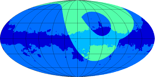
Figure 1: Galactic mask (dark blue lane) applied to the Archeops coverage (annular green region). The CMB mask is obtained by requesting the SFD brightness at 353 GHz to be $<0.5$ MJy.sr^-1. The Mollweide projection of the celestial sphere is in Galactic coordinates centered on the Galactic anti–center. Gridding on the full sky map is by 30 degree steps. The CMB analysis includes 20 % of the sky (dark green area) while Archeops covers $\sim$30 % of the sky. The previous analysis only covered 12 % of the sky above the 30 degree Northern parallel.

2.3 Map-making

The noise power spectrum of the Archeops TOIs is nearly flat with increasing power at very low time frequencies due to residuals from atmospheric noise, and at very high time frequencies due to the deconvolution from the bolometer time constants. To cope with these two features on the Archeops noise we have used an optimal (i.e. it achieves least square error on pixelised map) procedure called MIRAGE (Yvon & Mayet 2004 ) to produce maps for each of the detectors.

MIRAGE is based on a two-phase iterative algorithm, involving optimal map-making together with low frequency drift removal and Butterworth high-pass filtering. A conjugate gradient method is used for resolving the linear system. A very convenient feature of MIRAGE is that it handles classic experimental issues, such as corrupted samples in the data stream, bright sources and Galaxy ringing effects in the filtering and in the calculation of the noise correlation matrix.

Maps are computed with 7 arcmin. pixels (HEALPix $nside=512$) for each absolutely calibrated detector with their data time band–passed between 0.1 and 38 Hz. This corresponds to about 90 deg. and 20 arcmin. scales, respectively. The high–pass filter removes remaining atmospheric and Galactic contamination. The low–pass filter suppresses non–stationary high frequency noise.

About two thirds of the Archeops sky are observed with $\sim$20 to 60 samples per bolometer and per square degree and one third with a higher redundancy, about 75 samples per bolometer and per square degree. For illustration, Fig. 2 shows a map obtained from a weighted linear combination of the maps of each of the six most sensitive Archeops detectors. This map is smoothed with a 30 arcmin. gaussian beam and has a typical rms noise of 50 $\mu$K per 30 arcmin pixel.

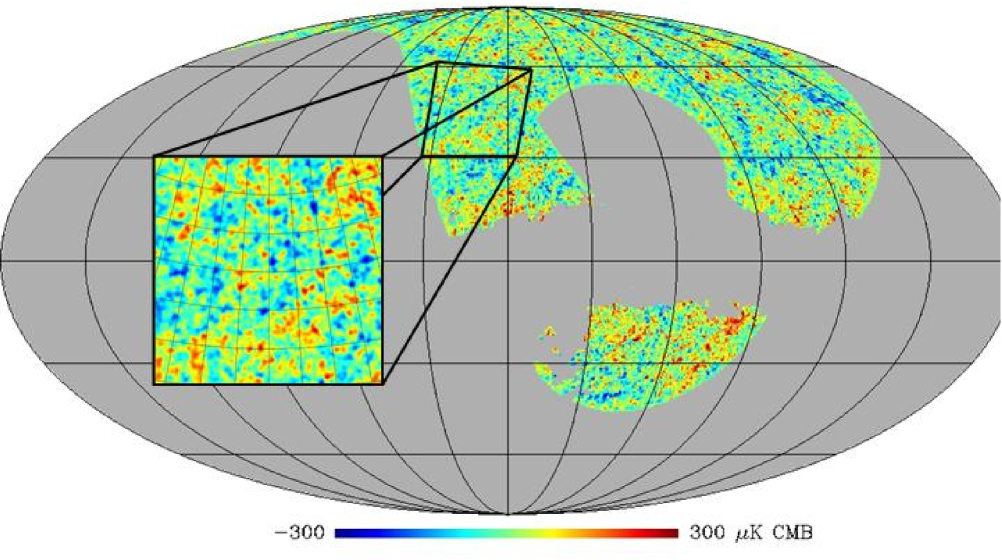
Figure 2: Archeops map of the CMB sky in Galactic coordinates centered on the Galactic anti-center after smoothing with a 30 arcmin. Gaussian. A patch of the sky of 30$\times$30 deg., with high redundancy and centered on ($l$, $b$) = (195,45) degrees is zoomed up. Gridding on the full sky map is by 30 degree steps, gridding on the zoomed patch is 5 deg. The Galaxy is masked as described above.

3 Power spectrum estimation

In this section, we present three methods, Xspect (Tristram et al. 2004 ), SMICA (Patanchon 2003 ) and power spectrum on the rings ($\Gamma_{m}$ hereafter) (Ansari et al. 2003 ) used for the determination of the angular power spectrum of the CMB temperature anisotropies with the Archeops data. Beforehand we detail the procedure we use to correct from beam smoothing and filtering effects as well as from inhomogeneous coverage.

We have thoroughly probed Xspect and SMICA with simulations which are described below. Results from both methods are included in this paper to cross validate the final results. The $\Gamma_{m}$ method is provided here to illustrate its potential in the estimation of the angular power spectrum directly from ring data and is more suitable to Planck-like data.

Xspect and SMICA are based on the so-called ‘pseudo-$C_{\ell}$’s estimators (Peebles 1973 ; Szapudi et al. 2001 ; Hivon et al. 2002 ) which directly compute the pseudo power spectrum from the spherical harmonics decomposition of the maps. These spectra are then corrected from the sky coverage, beam smoothing, data filtering, pixel weighting and noise biases.

A pseudo power spectrum $D_{\ell}$ is linked to the true power spectrum $C_{\ell}$ by

$$\widehat{D_{\ell}}=\sum_{\ell^{\prime}}M_{\ell\ell^{\prime}}p_{\ell^{\prime}}^{2}B_{\ell^{\prime}}^{2}T_{\ell^{\prime}}{\left\langle C_{\ell^{\prime}}\right\rangle}+{\left\langle N_{\ell}\right\rangle}\,\,\,.$$ (1)

where $M_{\ell\ell^{\prime}}$ is the mode-mode coupling matrix, $B_{\ell}$ is the beam transfer function describing the beam smoothing effect, $p_{\ell}$ is the transfer function of the pixelization scheme of the map describing the effect of smoothing due to the finite pixel size and geometry, $T_{\ell}$ is an effective transfer function that represents any filtering applied to the time ordered data, and ${\left\langle N_{\ell}\right\rangle}$ is the noise power spectrum.

In the following, the $M_{\ell\ell^{\prime}}$ matrix describes the mode-mode coupling resulting from the incomplete sky coverage and the weighting applied to the sky maps. We take into account the $p_{\ell}$ pixel transfer function due to the smoothing effect induced by the finite size of the map pixels. This function is provided in the HEALPix package (Gorski et al. 1999 ).

3.1 Beam smoothing effect

Most of the beams of the Archeops detectors have been measured on Jupiter to be elliptical. A few of them are irregular. Therefore, the effective beam transfer function must be carefully estimated for each bolometer. The beam transfer functions are computed from simulations using the Asymfast method detailed in (Tristram et al. 2004 ). This method is based on the decomposition of the beam into a sum of Gaussians for which convolution is easy in the spherical harmonic space (up to 12 Gaussians are used here). This allows us to deal with asymmetric beam patterns using the scanning strategy of the instrument. Figure 3 shows the beam transfer function for each of the Archeops detectors used in this analysis. They are estimated with a Monte-Carlo of 100 Asymfast simulations per bolometer. The beam transfer functions for the 143 GHz detectors are very similar and close to circular Gaussian. The 217 GHz detector beams are larger and more irregular, and smear-out more the high multipoles.

The Asymfast method produces negligible ($<$ 0.1 %) statistical uncertainties on the $B_{\ell}$ estimation. However, as the beam patterns have been measured on Jupiter maps they may differ from the effective beams on the CMB anisotropies. This comes mainly from uncertainties on the electromagnetic spectral dependence, far-side lobes, baseline subtraction and time constants, each of which estimated to be lower than 5%. For such systematics it is difficult to estimate their impact on the beam transfer function. As an illustration, we give conservative upper limits on the $B_{\ell}$ uncertainties by taking, as 1-sigma level error, a third of the difference between resulting transfer function from elliptical beams (Fosalba et al. 2002 ) and that from the Asymfast decomposition in multiple Gaussians. Fig. 6 shows the uncertainties on the $C_{\ell}$s due to the beam transfer function uncertainties. They are well below the statistical error bars.

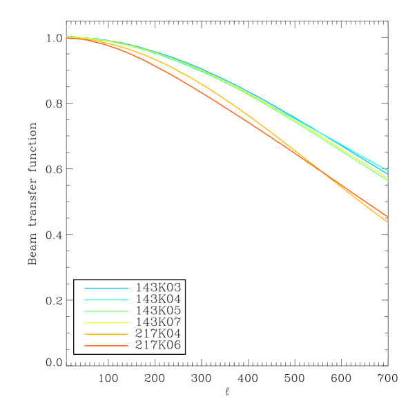
Figure 3: Beam transfer functions of the six most sensitive Archeops detectors computed using the Asymfast beam description.

3.2 Filtering and inhomogeneous coverage effects

Filtering leads to a preferred direction on the sky (the scanning direction) and so the assumption of isotropic temperature fluctuations implicitly done in Eq. 1 is not valid any more. However, to a first approximation, the bias on the CMB power spectrum due to the filtering of the time ordered data can be accounted for in the spherical harmonic space through the $T_{\ell}$ transfer function.

For this analysis we have performed two types of filtering associated with the destriping of the data discussed in Sect. 2.1 and with the band-pass filter applied to the data on the map making procedure.

The band-pass filter function $F_{\ell}$ is computed from 100 simulations of the CMB sky. The simulated maps are converted into timelines using Archeops pointing. These timelines are then filtered as the Archeops data. Subsequently, they are projected onto maps and the power spectrum of those is compared to the power spectrum obtained from maps of the same but unfiltered timelines.

Figure 4 shows in blue the band-pass filter function. It reaches 65 % at $\ell=10$ and remains above 85 % in the multipole range [25–700]. In our analysis, all bolometers are identically filtered and the difference between their pointing vectors is very small as these bolometers are distributed onto two rows separated by only $\sim$30 arcmin in the focal plane. We therefore assume an identical $F_{\ell}$ function for all detectors. Uncertainties on the estimation of the $F_{\ell}$ function are derived from the dispersion of the simulations.

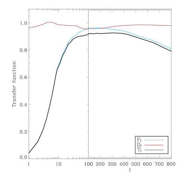
Figure 4: Archeops transfer functions: $F_{\ell}$ filter function (in blue), $D_{\ell}$ destriping transfer function (in red) and $T_{\ell}$ total Archeops transfer function (in black).

The transfer function associated with the destriping, $D_{\ell}$, has been computed using simulations and is shown in red on Fig. 4. The accurate determination of this function is difficult because the destriping procedure is non linear and CPU intensive. Thus, in order to be very conservative, we choose to take a third of the estimate of the function itself as the systematic error for it.

The total transfer function used for the Archeops pipeline $T_{\ell}=F_{\ell}\times D_{\ell}$ is plotted in black on Fig. 4. The uncertainties on the final power spectrum due to the errors on the $T_{\ell}$ function are represented on Fig. 6.

3.3 Xspect

The Archeops angular power spectrum has been computed using an extension of the ‘pseudo-$C_{\ell}$’ method to cross power spectra called Xspect (Tristram et al. 2004 ). Assuming no noise cross–correlation between different detectors, the noise term in Eq. 1 vanishes and each cross power spectrum, $A\neq B$, is an unbiased estimate of the $C_{\ell}$s. Pseudo cross power spectra can be easily corrected from inhomogeneous sky coverage, beam smoothing and filtering effects by extending Eq. 1 into:

$$\widehat{D_{\ell}^{AB}}=\sum_{\ell^{\prime}}M_{\ell\ell^{\prime}}^{AB}p_{\ell^{\prime}}^{2}B_{\ell^{\prime}}^{A}B_{\ell^{\prime}}^{B}T_{\ell}{\left\langle C_{\ell^{\prime}}^{AB}\right\rangle}$$ (2)

where the beam transfer functions $B_{\ell}$ for each bolometer and the transfert function $T_{\ell}$ are those previously described. The mode-mode coupling kernel $M_{\ell\ell^{\prime}}^{AB}$ is computed for each cross power spectra from the cross-power spectrum of the weighted masks. For the noise weighting scheme we consider a different noise weighted mask for each Archeops detector. This mask is constructed by multiplying the mask on Fig. 1 by the inverse of the noise variance on each pixel and is convolved by a 30 arcmin. Gaussian.

After correction, all cross power spectra ${\left\langle C_{\ell^{\prime}}^{AB}\right\rangle}$ are combined into a single estimate of the power spectrum, $\widetilde{C_{\ell}}$, by weighted averaging assuming the correlation between multipoles to be negligible. This last assumption is not completely true, as we can see some correlation at low multipoles on Fig. 7. Thus the estimate is not completely optimal but no measurable bias has been found in tests of Xspect on realistic simulations of Archeops data sets. Analytical estimates of the covariance matrix and of the error bars in the power spectrum are also given.

Xspect is designed to estimate both the angular power spectrum and its error bars even with incomplete sky coverage and mask inhomogeneities, as is the case with the present Archeops data. The approach has been validated with simulations including realistic noise and CMB temperature anisotropies. The noise timelines are simulated from an estimation of the Fourier power spectrum of the noise (Amblard & Hamilton 2004 ) for each of the photometric pixels. The CMB signal is simulated using the HEALPix software from the Archeops best-fit $\Lambda$CDM model (Benoît et al. 2003b ) convolved by the beam transfer function. Signal and noise are added into a single timeline which is filtered as the Archeops data and projected on the sky using the Archeops pointing.

Three sets of 1000 simulations have been computed for sky maps with HEALPix resolution $nside=512$ : a first one using an uniform weighting, a second one using a noise weighting scheme, and a third one with no noise added. Simulations were performed using the same optimal map-making method (Yvon & Mayet 2004 ) as the one used for the data.

From these simulations we have found that there is no bias at the 1% level in the estimation of the power spectrum. The analytical error bars provided by Xspect are also found to be above the standard deviation in the simulations by less than 10% and with a rms of 7%. Moreover, the noise contribution to the error bars on the simulated data and the Archeops data are in agreement within 5%. Hereafter, we will use the analytical estimates provided by Xspect for the error bars of the Archeops angular power spectrum excluding the sample variance contribution. The latter is computed from the dispersion of the simulations without noise and is added up to obtain the final error bars on the CMB angular power spectrum. Therefore, the sample variance contribution to the error bars is given by the best-fit Archeops model described in Benoît et al. 2003b .

As mentioned ealier, an improvement of about 10% on the error bars is obtained by using uniform weighting at low multipoles and a noise weighting scheme at high multipoles. Thus, in the following all power spectra presented are computed using uniform weighting up to $\ell<260$ and using a noise weighting scheme for $\ell\geq 260$.

3.4 SMICA

Using the filtering and beam transfer functions as well as the masks described in Sect. 3.1 and 3.2, we process the Archeops maps with a different estimation method of the CMB angular power spectrum: SMICA (Spectral Matching Independent Component Analysis) (Patanchon 2003 ).

A specificity of SMICA is its ability to estimate jointly the power spectra of several underlying components (including noise) assuming that the observed sky is a linear combination of components. In spherical harmonic space and in a matrix form, the model is :

$$x_{\ell m}=A\leavevmode\nobreak\ s_{\ell m}+n_{\ell m}$$ (3)

where $x_{\ell m}$ is a vector of spherical harmonics coefficients of the observed maps for each of the considered detectors; $A$ is the $N_{d}$ (number of detectors) $\times$ $N_{c}$ (number of components) mixing matrix which defines the amplitude of the different components in each observed map. The coefficients of $A$ are related to the electromagnetic spectra of the components and to the relative calibration between detectors. The spherical harmonic coefficients of the components and noise are stored in vectors $s_{\ell m}$ and $n_{\ell m}$.

SMICA is based on matching empirical auto- and cross spectra to their expected forms, as predicted by model (3) and by the statistical assumption of decorrelation between components. The mismatch is measured by a measure of divergence between the measured and modeled spectra which stems from the likelihood of a Gaussian stationary model. The adjustable parameters are: the power spectrum of each of the components (including CMB and noise) as well as the mixing matrix $A$. A complete description of SMICA is given in Delabrouille et al. 2003 ; Cardoso et al. 2002 ; Patanchon 2003 .

In the specific case of Archeops, spectral statistics are formed as follows. The spherical harmonic coefficients $x_{\ell m}$ are computed on the sky region which is common to all detectors using two different weighting schemes. For $\ell<260$, pixels are uniformly weighted. For $\ell\geq 260$, pixels are weighted proportionally to the number of data samples per pixel for the best detector. Band-averaged pseudo auto- and cross-power spectra are formed from these $x_{\ell m}$ and corrected for beam smoothing. If $Q$ bands are used, we obtain in this manner a set of $Q$ spectral matrices $\widehat{R}_{q}$ ($q=1,\ldots,Q$), each of size $N_{d}\times N_{d}$. Next, we choose which parameters should be be estimated (power spectra for CMB and possibly other components, all or parts of the coefficients, noise levels), collect all these parameters into a vector $\theta$ and denote $R_{q}(\theta)={\left\langle\widehat{R}_{q}\right\rangle}$ the expected value of the spectral matrices for a given value of $\theta$ (this is easily computed from model (3)). The SMICA algorithm estimates the unknown parameters by minimizing the spectral mismatch

$$\phi(\theta)=\sum_{q}w_{q}K(\widehat{R}_{q},R_{q}(\theta))$$ (4)

where $w_{q}$ is the number of independent $a_{lm}$ in the $q$th spectral band and where the mismatch measure $K(\cdot,\cdot)$ between two positive matrices is defined as $K(M_{a},M_{b})=\frac{1}{2}\left(\mathrm{trace}(M_{a}M_{b}^{-1})-\log\det M_{a}M_{b}^{-1}-N_{d}\right)$ (with this choice, the estimated parameter $\widehat{\theta}=\arg\min\phi(\theta)$ is a maximum likelihood estimate as shown in Delabrouille et al. 2003 ). The resulting estimated power spectra are then corrected from partial coverage and filtering effects using the MASTER formalism described in Sect. 3.2.

In order to evaluate error bars and possible biases, we have performed 500 realistic simulations of Archeops data. The data model includes synthetic CMB emission (observed with the same scanning strategy as used by Archeops) and noise for each detector. Application of SMICA to these simulated data has not shown any measurable bias.

Error bars for the estimated power spectra can also be obtained analytically from the Fisher information matrix. They have been compared to the dispersion found in the Monte-Carlo simulations. Analytic error bars on the CMB power spectrum are found to be slightly underestimated (about 10% on average). In the following, we use the analytic error bars corrected from the factor measured in the simulations.

3.5 CMB power spectrum on the rings

A third approach based on one-dimensional properties of the CMB inhomogeneities on rings has been performed on Archeops data (Ansari et al. 2003 ; Plaszczynski & Couchot 2003 ). It has been made possible by the Archeops sky scanning strategy, which scans quasi circles on the sky. The fact that we directly use TOI information with no requirement of projection on maps of the sky makes this method complementary to the two previous ones.

$\Gamma_{m}$ is defined as the Fourier power spectrum of the signal on a sky ring. For a ring of colatitude $\Theta$, the relation between $\Gamma_{m}(\Theta)$ and the $C_{\ell}$ (Delabrouille et al. 1998 ) follows:

$$\Gamma_{m}(\Theta) = \sum_{\ell=|m|}^{\infty}C_{\ell}T_{\ell}B_{\ell}^{2}{\cal(P)}_{\ell m}^{2}(\Theta)\ .$$ (5)

where $T_{\ell}$ is the transfer function for the destriping and filtering, $B_{\ell}$ is the beam transfer function and ${\cal(P)}_{\ell m}$ are the Legendre polynomials.

Rings are built for each bolometer from the TOIs by using the pointing information. They are then analysed by pairs. For each ring pair ($i-1$,$i$), whenever measurements taken at the same angular phase $\phi$ are separated on the sky by less than $0.1$ degree, we define a “signal” $S_{i}(\phi)$ and a “noise” $N_{i}(\phi)$ as respectively the half sum and half difference of the measurements from each rings.

Once these quantities are computed ring per ring, we analyse $S$ and $N$ in two ways. On the first hand, we compute the difference of the mean values of their Fourier spectra (that we call the $\Gamma_{m}$ analysis). On the other hand, the average of the auto-correlation functions for each pair is computed and then Fourier transformed to obtain the $\Gamma_{m}$ power spectrum. In both cases a Galactic mask similar to that described in Sect. 2.2 is applied. In addition since the autocorrelation approach needs all the low frequency drifts to be properly removed, we apply a cross-scan destriping (Bourrachot 2004 ). Since the noise directly pops-up from the data themselves, no simulation is needed in these approaches.

The error bars on the $\Gamma_{m}$ power spectrum are computed from the dispersion on the Fourier transform across rings and then propagated to obtain the uncertainties on the angular power spectrum.

4 Main results

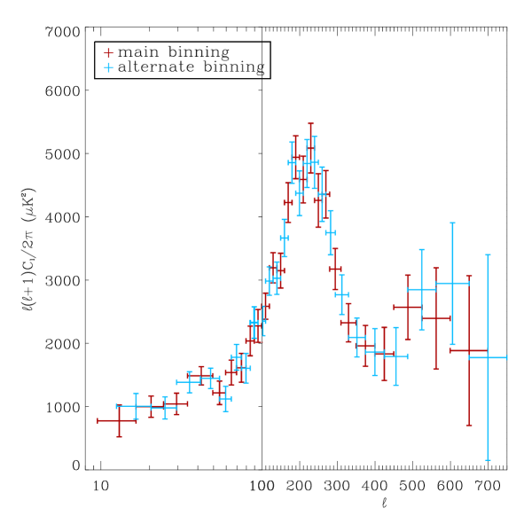
Figure 5: Archeops temperature angular power spectrum obtained using the Xspect method. A mixing of log-linear scales is presented to improve the readibility of the figure both on the Sachs–Wolfe plateau and on the acoustic peaks regions. Two intertwined and therefore not independent binnings (red and blue) are represented.

The analysis presented in this paper uses the six most sensitive Archeops bolometers, four at 143 GHz and two at 217 GHz with instantaneous sensitivities ranging from 93 to 207 $\mu{\mathrm{K}}_{\mathrm{C}MB}\,{\mathrm{s}}^{\frac{1}{2}}$. Note that those instantaneous sensitivities are better, by a factor of at least five, than those of the WMAP satellite mission detectors (Bennett et al. 2003 ) and a factor 2 to 4 worse than the nominal ones expected for the Planck–HFI instrument. We consider 20 % of the sky by applying the Galactic mask presented in Sect. 2.2.

Table 1 presents the angular power spectrum measured by Archeops. Results for the Xspect and SMICA methods are both given as they are based on different assumptions on the data model.

4.1 Archeops temperature angular power spectrum using Xspect

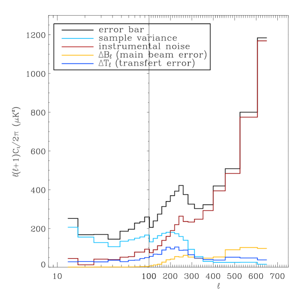
Figure 6: Detailed description of the statistical error bars (in black) on the Archeops angular power spectrum obtained with Xspect in terms of sample variance (in cyan) and instrumental noise (in red). In addition, systematic errors on the angular power spectrum estimation due to uncertainties on the filter (in blue) and beam smoothing function (in yellow) are shown (see Sect. 3).

Figure 5 shows the Archeops CMB angular power spectrum obtained using the Xspect method for two intertwined binnings (blue and red). These binnings correspond to two sets of overlapping and shifted window functions which lead to two non–independent estimates of the CMB angular power spectrum. A mix of logarithmic and linear scales in multipole space is presented to improve the readibility of the figure both on the Sachs–Wolfe plateau and on the first two acoustic-peaks clearly detected by Archeops. Two different weighting schemes are combined to produce the smallest error bars. At low $\ell$ multipoles a uniform weighting is preferred whereas for high $\ell$s the sky maps for each detector are noise weighted by using $w_{p,d}=1/\sigma_{p,d}^{2}$ where $\sigma_{p,d}^{2}$ is the variance of the pixel $p$ of the sky map from the detector $d$. The two schemes yield identical results around the mixing point, $\ell\simeq 260$ and they are joined in order to minimize the final error bars.

Figure 7: Error covariance matrix of the Archeops angular power spectrum computed using the Xspect method. The correspondence between bin number and multipole range is indicated in Tab. 1. The off-diagonal terms are less than 12 %

Figure 6 shows a detailed description of the statistical error bars (in black) on the Archeops angular power spectrum in terms of sample variance (in cyan) and instrumental noise (in red). Sample variance is deduced from the set of simulation without noise. It corresponds to the uncertainty on the model that is induced by the fact that we can only look at a part of one realisation of the sky. Sample variance dominates for $\ell<100$ and contributes to 50% or more of the total statistical error up to $\ell\sim 200$. Systematic errors due to uncertainties on the filter (in blue) and beam smoothing function (in yellow), which were computed as discussed in Sect. 3, are well below the statistical errors.

Figure 7 shows the absolute value of the normalised error covariance matrix of the Archeops angular power spectrum for the binning shown in red on Fig. 5. The correspondence between bin number and multipole range is indicated in Tab. 1. This matrix was computed using the simulations described in section 3.3 and provides the absolute correlation between multipole bins. The off-diagonal terms are less than 12 %, and therefore the $C_{\ell}$ estimates can be considered as roughly uncorrelated across bins on multipole space.

4.2 Archeops temperature angular power spectrum using SMICA

To apply the SMICA method to the Archeops data we choose to estimate two components (number required by the data: see figure 9 and related comments) corresponding to the CMB anisotropies and to unidentified residuals from foregrounds. The mixing matrix is simultaneously estimated allowing for recalibration of individual detectors against the most sensitive photometric pixel at 143 GHz.

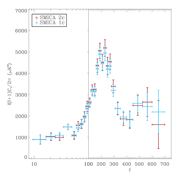
Figure 8: Archeops temperature angular power spectrum obtained using the SMICA method for one (in red) and two (in blue) components. A mixing of log-linear scales is presented to improve the readibility of the figure both on the Sachs–Wolfe plateau and on the acoustic peaks regions.

We find that CMB anisotropies are clearly detected for all the bolometers. A second component, much weaker in amplitude, is significant only in the 217 GHz maps. This component is thought to be a weak residual of foreground subtraction (see Sect. 5.3 for a more detailed discussion). Figure 8 shows in red the estimated CMB power spectrum with SMICA assuming two components.

To assess the impact of the second component, we run SMICA assuming a single physical component in the Archeops maps, meant to be the CMB anisotropies. For this second analysis, we fix the CMB mixing parameters to the values derived from the dipole calibration, allowing the direct comparison with Xspect. Figure 8 shows in blue the CMB power spectrum obtained in this way.

The fit of the estimated model to the data is quantified by the lowest possible value $\phi(\widehat{\theta})=\min_{\theta}\phi(\theta)$ of the spectral matching criterion Eq. (4). If the model of observations is correct (i.e. includes the probability distribution of the data), then $\phi(\widehat{\theta})$ should be statistically small. A finer picture is obtained by splitting the overall fit of $\phi(\widehat{\theta})$ into its components $w_{q}K(\widehat{R}_{q},R_{q}(\widehat{\theta}))$ as a function of the multipole bin $q$. Figure 9 shows the spectral adjustment of the best one-component model and of the best two-component model. The adjustment is much better with two components than with a single component, indicating that a second component is required by the data.

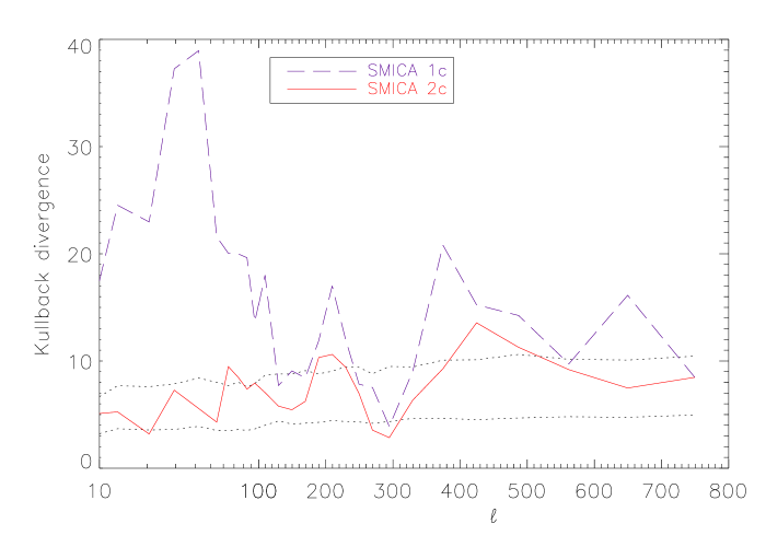
Figure 9: Rescaled spectral fit as function of the multipole. The dashed line is the fit for 1 component, the solid line curve is for 2 components. The dotted lines are the bounds of the 68% confidence interval estimated in simulations of the two-component model. Note how a two-component model brings the spectral mismatch within the statistical error bounds, showing that in addition to the CMB anisotropies a second component is required by the data mainly at low spatial frequency ($\ell<100)$.

Blind estimate for two components allows to separate systematic residuals in the two 217 GHz maps at the cost of some small increase in the CMB power spectrum error bars. The errors on the estimated CMB mixing parameters (bolometer intercalibration error) influence the error bars on the power spectrum estimate. The ratio between CMB power spectrum statistical error bars for the two and one component cases is about 20 % at low $\ell$ and 10 % at high $\ell$.

5 Discussion

The CMB angular power spectrum measured by Archeops as computed using Xspect and SMICA extends to a larger multipole range the results presented in (Benoît et al. 2003a ) and is in good agreement with them on the common multipole range reducing the error bars by a factor of three.

5.1 Consistency checks

Internal tests of consistency have been implemented in order to check the robustness of the results presented above. The Archeops CMB angular power spectrum has been computed for two different map resolutions ($nside=512,256$ corresponding to 7 and 14 arcmin pixels resp.) and we observe no significant differences between them. Furthermore, we have substantially varied the frequency intervals for the timeline bandpass filtering and no significant effect appears in the estimation of the angular power spectrum even at high multipoles. In addition, to check the consistency of the results between the two CMB channels (143 and 217 GHz) we have computed, using Xspect, the CMB angular power spectrum for only the four 143 GHz bolometers. Figure 10 shows this spectrum (in blue) compared to the one using the 6 most sensitive photometric pixels (in red). The spectra are in very good agreement, within the error bars, over the full multipole range. Using only the 143 GHz bolometers reduces significantly the sensitivity to the second acoustic peak but no systematic offsets are observed.

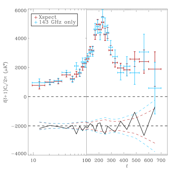
Figure 10: Xspect angular power spectrum using six detectors (in red) compared to the one obtained using only the four 143 GHz detectors (in blue). The difference between the two power spectra is given in the bottom plot (shifted by 2000) and are compared to the error bars (black dotted line).

As an extra consistency check, we compare in Fig. 11 the Archeops angular power spectrum obtained using Xspect (in red) with the one computed with 2-components SMICA method (in blue). The difference between the two power spectra, given in the bottom plot, is well below the error bars (red and blue dotted line). Detailed discussion of this issue is presented in Sect. 5.3.

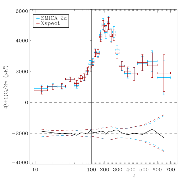
Figure 11: Archeops angular power spectrum using Xspect (in red) and using SMICA (in blue). The difference between the two power spectra is given in the bottom plot (shifted by 2000) and are compared to the error bars (blue and red dotted line). See text for details.

5.2 Archeops temperature angular power spectrum on the rings

We show on Fig. 12 the Fourier spectra obtained through the use of the two ring analysis methods described in Sect. 3.5 for the best Archeops bolometer at 143GHz. These analyses are in agreement within the error bars and show a clear detection of the first acoustic peak. These results indicate that the processed timelines contain no obvious spurious feature at a particular time frequency.

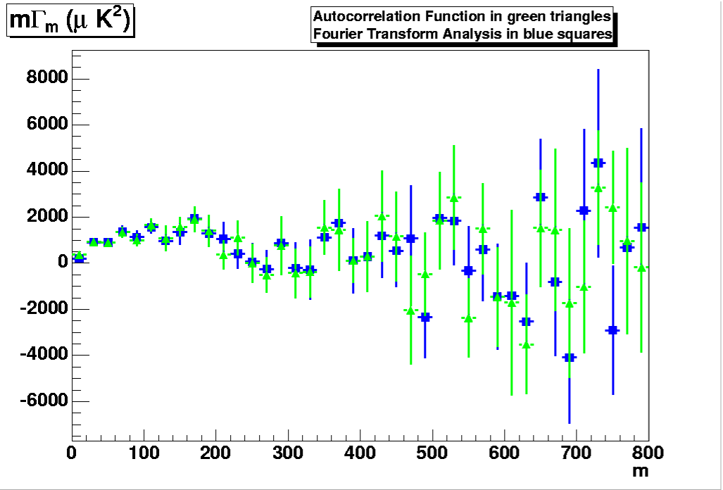
Figure 12: Fourier spectra obtained through the use of the two methods described in Sect. 3.5 for the best Archeops bolometer at 143GHz. These analyses are in agreement within the error bars.

5.3 Contamination from foregrounds

As any balloon-borne experiment, Archeops is exposed to the fluctuations of the atmospheric emission. Moreover the Galactic emission at 143 and particularly at 217 GHz is low but not negligible. Even if a careful decorrelation to suppress ozone and dust spurious emissions has been performed (see Sect. 2.2), the residuals from this decorrelation are a potential source of systematic errors in the determination of the CMB angular power spectrum.

The Galactic dust contribution must be much weaker at high Galactic latitudes. To assess the level of Galactic residuals, we have computed the angular power spectrum of the Archeops data using only the Northern part of the Archeops sky coverage. Figure 13 shows the estimate of the angular power spectrum for the Galactic mask described in Sect. 2.2 (in red) and for high positive Galactic latitudes: $b>+20\rm\,deg.$ (in blue) using Xspect. The differences between the two power spectrum estimates, shown in the bottom plot, are significantly smaller than the error bars associated to them. We conclude from this that the residual dust emission in the CMB angular power spectrum obtained from the Archeops data is small compare to the statistical errors in the multipole range $17\leq\ell<700$. The multipole bin $10\leq\ell<17$ shows a more important contimation from dust residual emission but still at the levels of the statistical and systematic uncertainties. For $\ell<10$ we found that the dust contamination was significant and therefore this multipole range was not included in this paper. The same test has been performed using SMICA and leads to identical conclusions.

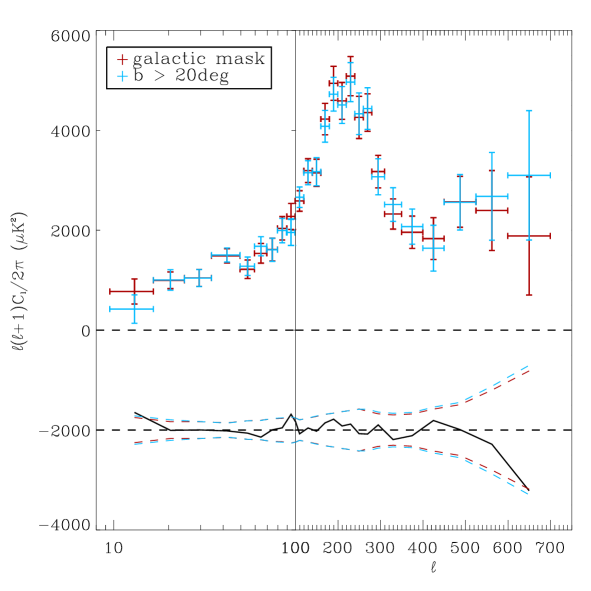
Figure 13: Xspect Archeops power spectrum computed for the Galactic mask described in Sect. 2.2 (in red) and for $b>20$ (in blue). The difference between the two estimates is given in the bottom plot (shifted by 2000) and compared to the error bars (blue and red dotted line).

To fully assess the residual contamination to the Archeops data from dust and atmospheric emissions we have performed two independent tests based on Xspect and SMICA respectively.

First, using the Xspect method we can cross-correlate the sky maps at 143 and 217 GHz used for the $C_{\ell}$ estimation with the sky maps of the 353 GHz Archeops detectors. The observed emission on the latter is dominated by dust and atmospheric emission and to first order we can neglect the CMB emission. Thus from this cross correlation, we can obtain an estimate of the residual foreground contribution to the Archeops CMB angular power spectrum computed with Xspect. The results from this analysis are shown on Fig. 14. The estimated contamination (in red) remains significantly below the statistical errors (in black) over the full multipole range except for the first multipole bin ($\ell$=[10-17[) for which the contamination is still smaller than the statistical error bar.

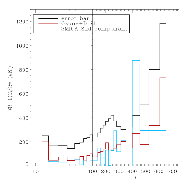
Figure 14: Atmospheric and Galactic dust residual emissions on the Archeops 143 and 217 GHz maps. In red, the residual foreground emission computed by cross-correlating these maps with the 353 GHz maps using the Xspect method. In blue, the residual foreground emission obtained from the second component detected by the SMICA 2 components analysis of the Archeops data. In black, we plot for comparison the error bars of the Archeops CMB angular power spectrum.

As discussed in Sect. 4.2 we have performed, using SMICA, a two component analysis of the Archeops six best photometric pixels. The first component on this analysis was identified as CMB emission whereas the second as the spurious residual foreground emission. This is significant only for the 217 GHz bolometer maps. This component is mainly due to residual atmospheric emission left behind after the linear decorrelation. This estimation is represented in Fig. 14, in blue, and can be compared to the foreground residual contamination estimated with Xspect at high multipoles. The SMICA estimate is of the same of order of magnitude and oscillates for $\ell>200$. These oscillations come from the uncertainties on the estimation of the second component which are well reflected on the error bars obtained for it. This could be due to correlated noise between the 217 GHz maps which would not be present in the residual foreground estimate obtained using Xspect. Further, this conclusion is reinforced by the fact that this contribution does not seem to be fully additive as expected from the SMICA model.

From the above results we can conclude that the Archeops CMB angular power spectra obtained using Xspect and SMICA are fully compatible if we take into account the residual atmospheric contamination which is in any case well below the statistical error bars as shown in Fig. 15. We have plotted the differences between the Archeops CMB angular power spectra computed with SMICA 1 and 2 component (in blue), SMICA 1 component and Xspect (in black), and SMICA 2 components and Xspect (in red). For comparison the statistical error bars are shown (black dashed line). This figure visually confirms the fact that the contamination from foregrounds on the Archeops CMB angular power spectrum is well below the error bars. This analysis of the foreground contamination validates our choice of the galactic mask described in Sect. 2.2.

Finally, the contribution from point sources is negligible in the multipole range considered here (see paper I).

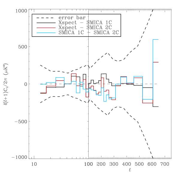
Figure 15: Differences between the Archeops CMB angular power spectra computed with SMICA 1 and 2 component (in blue), SMICA 1 component and Xspect (in black), and SMICA 2 components and Xspect (in red). For comparison the statistical error bars are shown (black dashed line).

5.4 Comparison to the standard $\Lambda$-CDM cosmological model

To check the validity of our results and their agreement with previous cosmological observations we have compared the CMB angular power spectrum measured by Archeops to the best-fit $\Lambda$-CDM cosmological model presented in (Spergel et al. 2003 ). This model was derived from a combination of the WMAP data with other finer scale CMB experiments, ACBAR and CBI and is defined by $h=0.71992$, $\Omega_{b}h^{2}=0.02238$, $\Omega_{m}h^{2}=0.11061$, $\tau=0.11026$, constant n_s (0.05 Mpc)${}^{-1}=0.95820$ and normalization amplitude $A$ (0.05 Mpc) $=0.73935$.

In Fig. 16 we present the best-fit $\Lambda$-CDM cosmological model described above superimposed on the Archeops CMB angular power spectrum which is rescaled by a factor $1.07$ in temperature ($1.14$ in $C_{\ell}$). This factor has been computed by assuming that the differences between the Archeops data and the model are due to a global scaling factor for all angular scales which has been fitted to $1.07\pm 0.02$ with $\chi^{2}$ of 27/24 and probability $Q=0.72$. For this fit we have only considered the statistical error bars on the angular power spectrum.

We observe that the agreement between the rescaled Archeops data and the model is very good. Here the model can be thought of as a guideline summarising other CMB experiments at different frequencies, in order to show the overall consistency across the electromagnetic spectrum. The scaling factor can be explained by the uncertainties on the absolute calibration of the Archeops data which are 6% in temperature (12% in $C_{\ell}$). A more detailed analysis of this issue is reported to a forthcoming paper including the determination of cosmological parameters from the Archeops data as well as a comparison to other CMB observations at the map level.

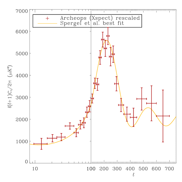
Figure 16: The Archeops temperature angular power spectrum rescaled by a factor $1.07$ in temperature superimposed on the $\Lambda$-CDM best-fit model by the WMAP team and presented in (Spergel et al. 2003 ).

6 Conclusion

Archeops was designed as a test-bench for Planck-HFI in terms of detectors, electronics, cryogenics and data processing. Archeops has demonstrated the validity of these technical choices two years ago by determining, for the first time and in a single balloon flight, the temperature angular power spectrum of the CMB from the Sachs–Wolfe plateau to the first acoustic peak ($15\leq\ell\leq 350$) using only two detectors.

In this paper we present an improved analysis of the Archeops data using the six most sensitive detectors and 20 % of the sky, mostly clear of foregrounds. Archeops has measured the CMB angular power spectrum in the multipole range from $\ell=10$ to $\ell=700$ with 25 bins, confirming strong evidence for a plateau at large angular scales followed by two acoustic peaks centered around $\ell=220$ and $\ell=550$ respectively.

The Archeops CMB angular power spectrum has been determined using two different statistical methods, Xspect and SMICA. The results from these two methods are in very good agreement with differences between them well below the statistical error bars. Furthermore, they allow a detailed analysis of the residual foreground contribution which is mainly due to atmospheric and Galactic dust emissions. The residual foreground emission on the Archeops data is small with respect to the error bars at all multipoles.

Finally, we have compared the Archeops CMB angular power spectrum to the best-fit $\Lambda$-CDM cosmological model presented in (Spergel et al. 2003 ) derived from a combination of the WMAP data with other smaller scale CMB experiments (ACBAR and CBI). We find that the Archeops data are in very good agreement with this model considering a rescaling factor to account for uncertainties on the absolute calibration.

A more detailed analysis for the determination of cosmological parameter with Archeops and other cosmological datasets will be discussed in a forthcoming paper. Furthermore, a comparison of the maps from Archeops, WMAP and other CMB datasets will be used to study the primordial nature of the measured CMB anisotropies from their electromagnetic spectrum.

All methods developed for this analysis will be implemented for the Planck–HFI data analysis. Even if Planck is less prone to systematic effects due to its space environment, the know–how acquired on Archeops data should prove useful in order to assess Planck final power spectrum.

				XSPECT			SMICA
bin	$\ell_{\mathrm{min}}$	$\ell_{\mathrm{max}}$	$\frac{\ell(\ell+1)}{2\pi}C_{\ell}$	total error	instrumental error	$\frac{\ell(\ell+1)}{2\pi}C_{\ell}$	total error	instrumental error	sample variance
1	10	16	774	251	45	899	217	11	206
2	17	24	998	167	12	1027	170	15	155
3	25	34	1043	168	41	999	149	22	127
4	35	49	1487	144	39	1486	131	26	105
5	50	59	1217	185	51	1081	173	39	134
6	60	69	1537	195	54	1561	189	48	141
7	70	79	1613	227	78	1619	206	57	149
8	80	89	2038	234	78	1978	223	67	156
9	90	99	2275	258	93	2451	242	77	165
10	100	119	2586	204	74	2639	201	71	130
11	120	139	3193	238	90	3221	232	84	148
12	140	159	3148	273	110	3234	274	111	163
13	160	179	4225	312	138	4358	312	138	174
14	180	199	4941	339	159	5050	356	176	180
15	200	219	4589	369	189	4506	377	197	180
16	220	239	5085	392	219	5183	388	215	173
17	240	259	4258	421	263	4340	402	244	158
18	260	279	4356	374	235	4538	365	226	139
19	280	309	3174	325	233	3385	302	210	92
20	310	349	2325	302	247	2351	298	243	55
21	350	399	1960	322	292	1862	309	279	30
22	400	449	1832	418	394	1825	399	375	24
23	450	524	2569	507	483	2487	465	441	24
24	525	599	2394	799	774	2649	676	651	25
25	600	699	1885	1183	1168	1595	1124	1109	15

Table 1: Archeops CMB power spectrum and statistical error bars (total, instrumental and sample variance) in $(\mu\mathrm{K_{CMB}})^{2}$ computed with Xspect and SMICA (with two components) for the best six photometric pixels.

- (1) Amblard, A., Hamilton, J.C., 2004, A & A, 417, 1189
- (2) Ansari, R., Bargot, S., Bourrachot, A. et al. 2003, MNRAS, 343, 552
- (3) Barkats, D., Bischoff, C., Farese, P. et al., 2004, ApJ, submitted, astro-ph/0409380
- (4) Bennett, C. L., Halpern, M., Hinshaw, G. et al., 2003, ApJ, 148, 1
- (5) Benoît, A., Ade, P., Amblard, A. et al., 2003a, A & A, 399, L19
- (6) Benoît, A., Ade, P., Amblard, A. et al., 2003b, A & A, 399, L25
- (7) de Bernardis, P., Ade, P. A. R., Bock, J. J. et al., 2000, Nat, 404, 955
- (8) Douspis, M., Riazuelo, A., Zolnierowski, Y., Blanchard, A., 2003, New Astronomy Review, 47, 755
- (9) Bourrachot, A., 2004, PhD Thesis, Université Paris Sud Orsay
- (10) Cardoso, J.-F., Snoussi, H., Delabrouille, J., Patanchon, G., 2002, EUSIPCO02 conference, astro-ph/0209466
- (11) Delabrouille, J., Gorski, K. M., Hivon, E., 1998, MNRAS, 298, 445
- (12) Delabrouille, J., Cardoso, J. F., Patanchon, G., 2003, MNRAS, 346, 1089
- (13) Finkbeiner, D., Davis, M., Schlegel, D., 1999, ApJ, 524, 867
- (14) Fixsen, D. J., Cheng, E. S., Cottingham, D. A. et al., 1994, ApJ, 420, 445
- (15) Fosalba, P., Doré, O., Bouchet, F. R., 2002, Phys. Rev. D, 65, 63003
- (16) Gorski K. M., Hivon E. & Wandelt B. D., 1999, in Proceedings of the MPA/ESO Cosmology Conference ”Evolution of Large-Scale Structure”, eds. A.J. Banday, R.S. Sheth and L. Da Costa, PrintPartners Ipskamp, NL, pp. 37-42 (also astro-ph/9812350)
- (17) Halverson, N. W., Leitch, E. M., Pryke, C. et al., 2002, ApJ, 568, 38
- (18) Hanany, S., Ade, P., Balbi, A. et al., 2000, ApJ, 545, L5
- (19) Hinshaw, G., Spergel, D. N., Verde, L. et al., 2003, ApJ, 148, 135
- (20) Hivon, E., Gorski, K. M., Netterfield, C. B. et al., 2002, ApJ, 567, 2
- (21) Lamarre, J. M., Puget, J. L., Bouchet, F. et al., 2003, NewAR, 47, 1017L
- (22) Lee, A. T., Ade, P., Balbi, A. et al., 2001, ApJ, 561, L1
- (23) Leitch, E., Kovac, J., Halverson, N. et al., ApJ, submitted, astro-ph/0409357
- Lineweaver et al. (1997) Lineweaver, C. H., Barbosa, D., Blanchard, A. et al., 1997, A & A, 322, 365
- (25) Macías–Pérez, J. F., Helbig, P., Quast, R. et al., 2000, A & A, 353, 419
- (26) Macías–Pérez, J. F., Bourrachot, A., Lagache, G. et al., 2005, in preparation
- (27) Madet, K., Maffei, B., Bock, J. J. et al., 2004a, in preparation
- (28) Miller, A. D., Caldwell, R., Devlin, M. J. et al., 1999, ApJ, 524, L1
- Netterfield et al. (1997) Netterfield, C. B., Devlin, M. J., Jarolik, N. et al., 1997, ApJ, 474, 47
- (30) Netterfield, C. B., Ade, P. A. R., Bock, J. J. et al., 2002, ApJ, 571, 604
- (31) Patanchon G., 2003, New Astron. Rev., 47, 871
- (32) Peebles P.J.E., Hauser M.G., 1974, ApJS, 28, 19.
- (33) Peebles P.J.E., 1973, ApJ, 185, 431
- (34) Plaszczynski S., Couchot F., 2003, MNRAS, submitted, astro-ph/0309526
- (35) Readhead, A., Myers, S., Pearson, T. et al., Science, 306:836–844, astro-ph/0409569
- (36) Rubino-Martin J. A., Rebolo, R., Carreira, P. et al., 2003, MNRAS, 341, 1084
- (37) Schlegel, D., Finkbeiner, D., Davis, M., 1998, ApJ, 500, 525
- (38) Sievers, J. L., Bond, J. R., Cartwright, J. K. et al., 2003, ApJ, 591, 599
- (39) Spergel, D. N., Verde, L., Peiris, H. V. et al., 2003, ApJ, 148, 175
- (40) Szapudi, I., Prunet, S., Pogosyan, D. et al., 2001, ApJ, 548, L115
- (41) Tristram, M., Hamilton, J.-Ch., Macías-Peréz, J. F. et al., 2004, Phys. Rev. D, 69, 123008
- (42) Tristram, M., Macías-Peréz, J. F., Renault, C. et al., 2004, MNRAS, in press, astro-ph/0405575
- (43) Yvon, D., Mayet, F., 2004, A & A, in press, astro-ph/0401505