Synchrotron Radiation From Radiatively Inefficient Accretion Flow Simulations: Applications to Sgr A*

Abstract

We calculate synchrotron radiation in three-dimensional pseudo-Newtonian magnetohydrodynamic simulations of radiatively inefficient accretion flows. We show that the emission is highly variable at optically thin frequencies, with order of magnitude variability on time-scales as short as the orbital period near the last stable orbit; this emission is linearly polarized at the $\sim 20-50\%$ level due to the coherent toroidal magnetic field in the flow. At optically thick frequencies, both the variability amplitude and polarization fraction decrease significantly with decreasing photon frequency. We argue that these results are broadly consistent with the observed properties of Sgr A* at the Galactic Center, including the rapid infrared flaring.

Subject Headings: Accretion, accretion disks – Galaxy: center

1 Introduction

The identification of magnetohydrodynamic (MHD) turbulence as a robust angular momentum transport mechanism has led to a new era in the study of accretion onto compact objects (see Balbus 2003 for a review). Numerical simulations can now demonstrate accretion without imposing an arbitrary anomalous viscosity. Although analytic steady state models provide an important framework for understanding the structure of accreting systems (e.g., Shakura and Sunyaev 1973; Narayan and Yi 1994; Blandford and Begelman 1999), a computational approach is required to capture the time-dependent, turbulent evolution of the flow. Simulations open up the time domain to theoretical study and should ultimately provide a more robust description of the observed features of accreting systems. Krolik and Hawley (2002) exploited this possibility by computing power spectra of quantities such as the accretion rate and Maxwell stress, both of which are presumably related to the bolometric output of the accretion flow. Hawley and Balbus (2002) carried out similar calculations, including estimating the characteristic frequency for synchrotron radiation in their simulations. Here we extend these calculations by explicitly calculating the radiative output from MHD simulations; for reasons explained below, we focus on synchrotron radiation. Our goal is to make general connections between numerical simulations and observations of accreting systems - we do not believe that the simulations yet contain sufficient physics to warrant detailed quantitative comparisons. We focus on observables such as polarization and fractional variability that are not as sensitive to the absolute value of the predicted flux (which is difficult to calculate for several reasons explained in §2).

We apply our results to observations of Sgr A*, the $\approx 3.6\times 10^{6}M_{\sun}$ massive black hole (MBH) at the center of our galaxy (Schödel et al. 2002; Ghez et al. 2003). Sgr A* is known to be remarkably faint: the canonical Bondi accretion rate estimate inferred using the observed gas density around the black hole predicts a bolometric luminosity $L\approx 0.1\dot{M}c^{2}\approx 10^{41}$ ergs s^-1, if radiation were produced with 10% efficiency (e.g., Baganoff et al. 2003). Instead, the observed luminosity is $\sim 10^{36}$ ergs s^-1 (Melia and Falcke 2001). This disagreement favors radiatively inefficient accretion flow (RIAF) models of Sgr A*, in which little of the gravitational binding energy of the inflowing matter is radiated away (e.g., Narayan et al. 1995; see Quataert 2003 for a review). Numerical simulations of RIAFs have shown that part of the reason Sgr A* is so faint is that the accretion rate is much less than the Bondi estimate (e.g., Stone & Pringle 2001; Hawley & Balbus 2002; Igumenshchev et al. 2003). This conclusion has been confirmed by observations of linear polarization in the mm emission from Sgr A* (Aitken et al. 2000; Bower et al. 2003; see, e.g., Agol 2000, Quataert & Gruzinov 2000, and Melia, Liu, & Coker 2000 for how the observed polarization constrains accretion models).

Sgr A* has been detected from the radio to the X-rays, with most of the bolometric power emerging at wavelengths near 1 millimeter (see, e.g., Melia & Falcke 2001 for a review of spectral models). The millimeter emission is significantly linearly polarized ($\sim 10\%$), consistent with synchrotron radiation (Aitken et al. 2000; Bower et al. 2003), while lower frequency radio emission is circularly polarized at the $\approx 0.1-1\%$ level (Bower et al. 1999). For the purposes of this paper, the most interesting aspect of the observations is the strong variability detected across the entire spectrum. X-ray flares with amplitudes from factors of a few up to $\sim 50$ have been detected on hour time-scales (Baganoff et al. 2001; Porquet et al. 2003). Flaring has also been seen in the infrared on time-scales as short as 10s of minutes (Genzel et al. 2003; Ghez et al. 2004). Order unity variability in the millimeter has been detected on longer time-scales (week to month; Zhao et al. 2003), with even lower amplitude, longer time-scale variations in the radio (Herrnstein et al. 2004). Occasionally, the radio emission can vary more rapidly as well, by $\sim 25\%$ over a few hours (Bower et al. 2002). In addition to variability in the total flux, the polarization in the radio exhibits variability as well (Bower et al. 2002, 2005). The origin of these variations is not fully understood. Analytic models generally interpret the X-ray and IR flares as emission due to transient particle acceleration close to the black hole (e.g., Markoff et al. 2001; Yuan, Quataert, & Narayan 2003, 2004; hereafter YQN03 and YQN04), although alternative interpretations exist (e.g., Liu & Melia 2002; Nayakshin et al. 2004).

In this paper we compute synchrotron radiation in an MHD simulation of a RIAF and discuss the results in the context of observations of Sgr A*. We focus our analysis on synchrotron radiation because it probably dominates the bolometric output of RIAFs at very low accretion rates (see, e.g., Fig. 5 of YQN04), and because of its clear applicability to Sgr A* (at least in the radio-IR). The synchrotron radiation is calculated “after the fact,” using the results of existing numerical simulations that do not incorporate radiation. This is self-consistent because energy loss via radiation is negligible and does not modify the basic dynamics or structure of the accretion flow.

The plan for the rest of this paper is as follows. In the next section (§2) we describe the simulations and our method for calculating synchrotron radiation. We then describe our results in §3. We begin by considering optically thin synchrotron emission (both total intensity and polarized), and then consider optical depth effects. Finally, in §4 we conclude and discuss our results in the context of observations of Sgr A*. Before describing our method in detail, it is worth noting some of the simplifications in our analysis. The simulations used in this paper are Newtonian and so do not account for relativistic effects near the black hole. In keeping with this simplified dynamics, we do not account for Doppler shifts or gravitational redshift when calculating the radiation from the flow. Lastly, the MHD simulations used here do not have detailed information about the electron distribution function, which we parameterize as a Maxwellian with a power-law tail.

2 Synchrotron Radiation from MHD Simulations

The specific simulation used in this paper is ‘Model A’ described in Igumenshchev et al. (2003). This is a Newtonian MHD simulation using the Paczynski-Wiita potential. The domain of the simulation is a set of 5 nested Cartesian grids, each of which has 32 elements in the x and y directions and 64 elements in the z direction. The smallest grid has elements that are 0.5 Schwarzschild radii ($R_{s}$) across, where $R_{s}=2G{M}/c^{2}$, and each successively larger grid has elements twice as large as the previous grid. All of the grids cover only two octants, both positive and negative z, but only positive x and y. The boundary conditions are periodic such that the x = 0 plane is mapped onto the y = 0 plane. At small radii the black hole is represented by an absorbing sphere and the central 2 $R_{s}$ are not evolved. At the outer boundary, $R=256R_{s}$, outflow boundary conditions are applied. Matter is injected continuously near the outer boundary with toroidal magnetic fields, allowing a steady state to be reached in which inflow into the grid is balanced by outflow out of the simulation domain and into the “black hole.” The flow has zero net poloidal magnetic field, and forms a geometrically thick convective accretion disk. There are no jets or significant mass outflow in the polar direction.

Since the simulation variables are dimensionless, length-scales and time-scales can be adjusted for any black hole mass. We present all physical quantities using $M=3.6\times 10^{6}M_{\odot}$, appropriate for Sgr A*. The data we use are taken from the roughly steady state portion of the simulation. We work with two different data sets. Data set 1 consists of 32 time-slices staggered by roughly 30 hours, which is the orbital period at about 50 $R_{s}$. These data include the full 3D structure of the flow (density, pressure, magnetic field strength, etc.). Since much of the emission comes from close to the BH, however, there is significant evolution between these time-slices. Data set 2 thus consists of about 10,000 time-slices separated by about $30$ sec, which corresponds to about 1/2 of the light-crossing time of the black hole’s horizon. These data were generated during a run of the simulation, and only contain information about the synchrotron radiation not the structure of the flow. Because of memory constraints, we could not retain the full 3D structure of the flow at all 10,000 of these timesteps. Instead, we rely on data set 1 (which has the full 3D structure, but sparser time sampling) to correlate the synchrotron emission with the structure of the flow and to determine optical depth effects. We use data set 2 to probe the optically thin emission and variability on all relevant time-scales.

There are several significant difficulties in using the simulations to predict synchrotron radiation. First, the density of gas in the simulation is arbitrary because the accretion rate is not fixed in physical units; that is, although the simulation describes the spatial and temporal evolution of the density, a single normalization parameter must be specified to compute physical gas densities. We adjust this density normalization so that the total synchrotron power is roughly that observed from Sgr A* (this depends on electron temperature; see below). Given the density normalization, the total pressure and magnetic field strength are uniquely determined.

The biggest uncertainty in our analysis is that the simulations only evolve the total pressure, while synchrotron radiation is produced by the electrons. Since RIAFs are collisionless plasmas, there is no reason to expect equal electron and ion temperatures or a thermal distribution of electrons (e.g., Quataert 2003). This is problematic because the synchrotron emission is sensitive to the exact electron distribution function, about which we have no information from MHD simulations. We account for this uncertainty as best as we can: we model the electrons using a thermal distribution with a non-thermal power-law tail. Given a total ion + electron temperature (pressure) $T_{tot}=T_{i}+T_{e}$ from the simulations, we determine the electron temperature using $T_{e}/T_{tot}$ as a free parameter of our analysis. We show results for several values of $T_{e}/T_{tot}$, focusing on $T_{e}/T_{tot}=1$ and $T_{e}/T_{tot}=1/4$. This roughly brackets the range of electron temperatures in recent semi-analytic models of emission from Sgr A* (e.g., YQN03). It is important to stress again that there is no compelling reason to expect the electron temperature to be everywhere proportional to the total temperature, but this is the best that we can do without solving separate ion and electron energy equations or carrying out kinetic simulations.

The choice of density normalization and electron temperature parameterization have a nontrivial impact on the predicted spectrum of the accretion flow. Figure Synchrotron Radiation From Radiatively Inefficient Accretion Flow Simulations: Applications to Sgr A* shows the optically thin synchrotron emission from a uniform plasma with $T_{tot}=2\times 10^{11}$ K for different choices of $T_{e}/T_{tot}$. For each calculation, we have adjusted the density to fix the total synchrotron power. To understand these results analytically, note that the peak frequency for relativistic thermal synchrotron emission (where $\gamma\propto T_{e}$) scales as

$$\nu_{peak}\propto B\gamma^{2}\propto q^{\frac{1}{2}}\left({T_{e}/T_{tot}}\right)^{2}$$ (1)

and the total synchrotron power scales as

$$P_{total}\propto B^{2}\gamma^{2}n_{e}\propto q^{2}\left(T_{e}/T_{tot}\right)^{2}\propto q^{3/2}\nu_{peak}$$ (2)

where $q$ is the density normalization parameter (i.e., $n_{e}\propto q$) and we assume fixed $\beta=P/(B^{2}/8\pi)$.

Given these uncertainties, our strategy is to choose several parameterizations for the electron temperature (via $T_{e}/T_{tot}$) and to adjust the density normalization such that the total synchrotron power is reasonable. Physically, this corresponds to electron temperatures $\sim 10^{10}-10^{11}$ K near the black hole and gas densities $\sim 10^{6}-10^{7}$ cm^-3 (see also the one-dimensional analytic models in YQN03). Because the simulations cannot uniquely predict the total synchrotron power or peak synchrotron frequency, our analysis focuses on observables that are less sensitive to the overall normalization of the emission, namely the variability and polarization. As we show later, the semi-quantitative conclusions of this paper do not depend that sensitively on the uncertainties in $T_{e}/T_{tot}$ and $q$, though detailed quantitative comparisons between simulations and observations are clearly premature.

In addition to considering a thermal electron population, we also account for a non-thermal tail in the electron distribution function. This power-law component is strongly motivated by models for the IR and X-ray emission from Sgr A* (e.g., Markoff et al. 2001; YQN04), and also is expected theoretically in models of collisionless plasmas. We assume that the power-law tail has a fraction $\eta$ of the electron thermal energy and a power-law index $p$ where $n(\gamma)\propto\gamma^{-p}$. We fix $p=3$ and choose either $\eta=0$ (no power-law component) or $\eta=0.05$ (see YQN03). We do not vary $p$ or $\eta$ in time or space, although such variation is likely inevitable due to transient events such as shocks and reconnection (and is certainly suggested by the IR and X-ray flaring from Sgr A*). As a result, our calculations of variability at high frequencies are likely lower limits, since they do not include variations in the accelerated electron population.

We compute the total synchrotron emission of data sets 1 and 2 assuming ultrarelativistic electrons (following Pacholczyk 1970, henceforth P70). We have checked that using the transrelativistic fitting formula of Mahadevan et al. (1996) yields almost identical results to the ultrarelativistic calculation for our problem. Given uncertainties in our viewing angle towards the accretion flow, we use a simple angle averaged emissivity to compute the emission from data set 2 (the high time sampled data set). We have assessed the validity of this approximation by computing the angle-dependent emission from data set 1 (which has the full 3D structure): the true flux is typically similar to that given by the angle-averaged formula to within $\approx 50\%$ (much less than the theoretical uncertainties due to the electron distribution function). The disagreement can be somewhat worse at very high frequencies ($\nu\mathrel{\mathchoice{\vbox{\offinterlineskip\halign{$\m@th\displaystyle\hfil#\hfil$\cr>\crcr\sim\crcr} }}{\vbox{\offinterlineskip\halign{$\m@th\textstyle\hfil#\hfil$\cr>\crcr\sim\crcr} }}{\vbox{\offinterlineskip\halign{$\m@th\scriptstyle\hfil#\hfil$\cr>\crcr\sim\crcr} }}{\vbox{\offinterlineskip\halign{$\m@th\scriptscriptstyle\hfil#\hfil$\cr>\crcr\sim\crcr} }}}10^{14}$ Hz) when one is on the exponential tail of the synchrotron emissivity.

In addition to calculating the total flux, we also calculate the linear polarization of synchrotron radiation in the simulations, again assuming ultrarelativistic electrons (P70; eqn 3.39). We also present several calculations including the effects of synchrotron self-absorption. For simplicity, we only calculate self absorption for viewers in the equatorial plane of the accretion flow. For our typical parameters ($T_{e}/T_{tot}$ and $q$), self-absorption effects become important below frequencies of a few hundred GHz. We account for self-absorption in the thermal component by calculating the optical depth along a ray using the emission coefficient and the thermal source function $S_{\nu}=2kT_{e}{\nu}^{2}/c^{2}$. The intensity along each ray is then given by adding up the optically thin emission from each grid point along the ray, weighted by $\exp(-\tau)$. Note that power-law electrons are omitted from this calculation, but each polarization mode is calculated separately so we can determine the polarization at both optically thick and thin frequencies.

We assume that at each time the observed emission is given by the steady state solution to the radiative transfer equation given the temperature, density, etc. of the accretion flow at that time. This is likely to be a reasonable approximation except for very short time-scale variability, and for emission from radii where the velocity of the gas approaches the speed of light (these limits are, of course, of considerable interest, but relaxing the steady state assumption is a significant effort beyond the scope of this work). In keeping with the Newtonian dynamics in the simulations used here, we also do not include gravitational redshift or Doppler shifts.

It is important to point out the effects of finite spatial resolution on our calculations. High frequency thermal synchrotron emission is produced primarily at small radii close to the black hole, where the temperature and magnetic field strength are the largest. The spatial resolution in this region is $0.5R_{s}$, so that at the last stable orbit ($3R_{s}$), there are a rather small number of grid points. We find that the thermal synchrotron flux at high frequencies (at and above the thermal peak) and the location of the peak are often determined by emission from a small number of grid points. As a result, the spatial resolution is not quite sufficient to accurately calculate the highest frequency synchrotron emission. This is likely to be a generic problem in calculating emission from simulations given resolution constraints. It is particularly acute above the thermal peak because the emission there is exponentially sensitive to $B$ and $T_{e}$. By contrast, below the thermal peak the emission is always well determined because it comes from a larger range of radii. As a check on how sensitive our results are to the inner few Schwarzschild radii, we have assessed how the emission from the flow changes if we only consider emission from outside (say) 4 or 6 $R_{s}$. We find that, although the overall amplitude of the flux at very high frequencies decreases, our primary conclusions regarding fractional variability and polarization (as enumerated in §4) are essentially unchanged. Thus we believe that these results accurately reflect the underlying dynamics of the accretion flow.

3 Results

To begin we present results for unpolarized synchrotron emission, without taking into account the effects of synchrotron self-absorption. We then discuss the polarization of the emission and the effects of synchrotron self-absorption. For some of the frequencies considered below it is not self-consistent to ignore self-absorption, but we do so initially to illustrate general points about synchrotron emission from the flow.

3.1 Optically Thin Emission

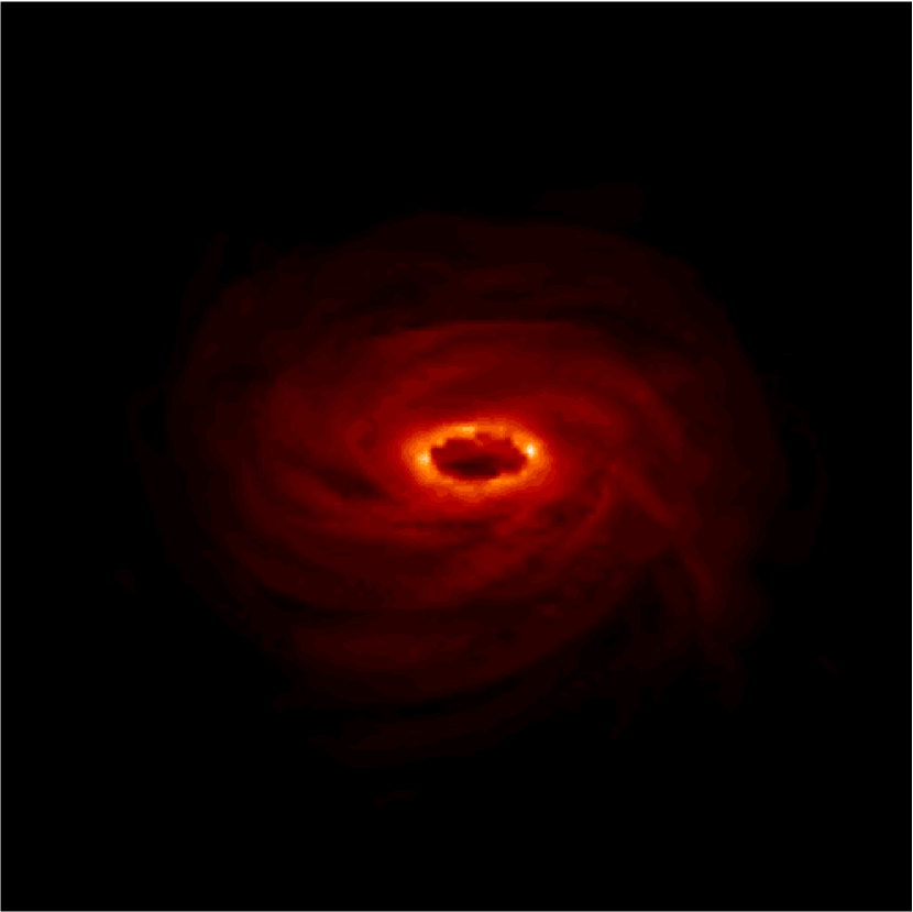
Figure 2: An image of the central 16 $R_{s}$ at a particular time-slice for $\nu\approx 450$ GHz, near the peak of the thermal emission. The intensity scale is logarithmic and the brightest area is in the equatorial plane near the last stable orbit, where the density, temperature, and magnetic field strength are the largest. For $\nu\ll 450$ GHz (below the thermal peak), the emission is much less centrally concentrated.

To become familiar with the emission it is useful to examine a time-slice and ‘see’ what the flow would look like if it could be resolved with an array in the sub-mm. This is shown in Figure 2 for a typical time-slice, as viewed from an arbitrary angle off of the plane at $\nu\approx 450$ GHz, which is near the peak in the thermal emission (see Fig. 7). We only show the central 16 $R_{s}$, which is by far the dominant emission region (the intensity plot in Fig. 2 is logarithmic). Most of the emission originates close to the central hole, in the equatorial plane, rather than, for instance, in polar outflows or jets, which do not appear in this simulation. This structure changes somewhat from time-slice to time-slice but the prominence of an equatorial region near the hole is common to all. At lower frequencies, where $\nu\ll\nu_{peak}$, large radii are more important and so the emission is much less centrally concentrated. Note that the calculations shown in Figure 2 do not include any General Relativistic photon transport (or even obscuration by the BH), which may give rise to unique signatures in the observed image (e.g. Falcke, Melia, & Agol 2000). Nonetheless, these calculations are encouraging because the emission arises so close to the hole, where GR effects would indeed be important.

Figure 3 shows the variability of the emission with time at three representative frequencies, from the radio to the IR. The calculations are for $T_{e}/T_{tot}=1/4$ and a power-law tail with $\eta=0.05$. The $\nu=10$ GHz and $\nu=80$ GHz emission are produced by the thermal component, while the $\nu=81.9$ THz emission (K-band IR) is produced by the non-thermal tail. The most striking feature of these results is the strong variability of the emission with time. The flux varies by up to an order of magnitude, often on time-scales as short as an hour. Figure 3 also shows that the amplitude of the variability increases, and the time-scale for variability decreases, at higher photon frequencies. This is because higher photon frequency emission originates closer to the hole where the dynamical time-scales are shorter. In addition, we find that variability of the flow parameters in the inner region is larger than the variability at large radii, accounting for the fact that the higher frequency emission that originates close to the hole is more variable.

To demonstrate the origin of this variability, Figure 4 shows how the flux at 100 GHz varies on long time-scales, as compared with the magnetic field strength ($|B|$), temperature ($T_{e}$), and density ($n_{e}$), averaged from 2 to 6 $R_{s}$. It is clear that the variability is primarily due to changes in the magnetic field strength, with fluctuations in temperature and density being less important (the correlation coefficients between $\nu L_{\nu}$ and $B$, $n$, and $T$, are 0.93, 0.66, and 0.57, respectively). Note that because the flow has $\beta\sim 10-100$, even large changes in the magnetic field strength do not necessarily lead to appreciable pressure or density changes, though they do cause significant variability in the synchrotron emission.

In the previous section we emphasized that the predicted emission depends on how we parameterize the electron temperature and distribution function. Figure 5 contrasts these different parameterizations in terms of the variability of the flow on different time-scales and at different photon frequencies. Figure 5 displays the power in Fourier components corresponding to one day and one hour periods, normalized to the mean flux (see caption for details). On hour time-scales the two models with purely thermal electrons look very similar, except that the variability at a given frequency is smaller for the model with hotter electrons. The reason for this is that higher electron temperatures imply that at a given photon frequency the emission arises from larger radii (so that $B$ is smaller), where the dynamical timescales are longer and thus the short time-scale ($\sim$ hour) variability is weaker.

Figure 5 also shows that higher photon frequency emission is significantly more variable than lower photon frequency emission on hour time-scales. This is because the lower photon frequency emission includes significant contributions from large radii where the orbital time-scales that govern the variability of the flow are $\gg 1$ hour. The trend of increasing variability with increasing photon frequency is present, but noticeably less dramatic, on day time-scales. This is simply because most of the radii that contribute to the observed emission have orbital periods $\mathrel{\mathchoice{\vbox{\offinterlineskip\halign{$\m@th\displaystyle\hfil#\hfil$\cr<\crcr\sim\crcr} }}{\vbox{\offinterlineskip\halign{$\m@th\textstyle\hfil#\hfil$\cr<\crcr\sim\crcr} }}{\vbox{\offinterlineskip\halign{$\m@th\scriptstyle\hfil#\hfil$\cr<\crcr\sim\crcr} }}{\vbox{\offinterlineskip\halign{$\m@th\scriptscriptstyle\hfil#\hfil$\cr<\crcr\sim\crcr} }}}1$ day, and thus are significantly variable on $\sim$ day time-scales. Finally, Figure 5 shows that non-thermal emission begins to dominate thermal emission at $\nu\approx 10^{12}-10^{13}$ Hz. In addition, the models with pure thermal emission are more variable than those with non-thermal emission at these frequencies; this is because $\nu\mathrel{\mathchoice{\vbox{\offinterlineskip\halign{$\m@th\displaystyle\hfil#\hfil$\cr>\crcr\sim\crcr} }}{\vbox{\offinterlineskip\halign{$\m@th\textstyle\hfil#\hfil$\cr>\crcr\sim\crcr} }}{\vbox{\offinterlineskip\halign{$\m@th\scriptstyle\hfil#\hfil$\cr>\crcr\sim\crcr} }}{\vbox{\offinterlineskip\halign{$\m@th\scriptscriptstyle\hfil#\hfil$\cr>\crcr\sim\crcr} }}}10^{12}-10^{13}$ Hz is near or above the peak in the thermal synchrotron emission (see Fig. 7), and so the flux is exponentially sensitive to variations in the flow parameters. Of course, the flux (and the variable flux) in the non-thermal tail at high frequencies is much larger than that produced by the thermal electrons, but the normalized variability is smaller.

3.2 Linear Polarization

We have also computed the net linear polarization of synchrotron emission in the simulation (neglecting Faraday rotation and optical depth effects; the latter are considered in the next section). The results are shown as a function of frequency in Figure 6 for all of the time-slices in data set 1 (each of which is separated by about 30 hours); for these calculations we chose to view the flow 30 degrees off of the equatorial plane, set $T_{e}/T_{tot}=1/4$, and included a non-thermal tail with $\eta=0.05$. As Figure 6 shows, the magnitude of the linear polarization is substantial, typically $30-40\%$. There is some variation with frequency, though it is not particularly dramatic. The polarization vector lies perpendicular to the equatorial plane. It arises due to the coherent toroidal magnetic field in the flow, analogous to the polarization of synchrotron radiation in the Galaxy (e.g., Beck 2001). The polarization would be larger ($\approx 60\%$; see Fig. 8) if we viewed the flow edge-on, while it would vanish for face-on viewing angles. Note also that there is appreciable variability in the magnitude of the polarization, roughly order unity changes on day to week time-scales. The variability is somewhat larger at high frequencies, again because this emission arises closer to the black hole.

3.3 Synchrotron Self-Absorption

In the previous sections we have assumed that the synchrotron emission is optically thin at all frequencies of interest. This assumption is incorrect at low frequencies where synchrotron self-absorption becomes important and the emission becomes optically thick. In this section we present initial results on the emission and variability at optically thick frequencies, leaving a more comprehensive discussion to future work. We have computed the total flux as a function of frequency including self-absorption for the case when the flow is viewed in the equatorial plane, perpendicular to the rotation axis (see §2 for the method); we considered thermal electrons only and took $T_{e}/T_{tot}=1/4$. The top panel in Figure 7 shows the average and RMS emission both with (solid) and without (dashed) optical depth effects, while the bottom panel shows the normalized RMS variability for these two cases. The averages and RMS are taken over all 32 time-slices (data set 1) for which we have the full 3D structure necessary to compute optically thick emission. Since these time-slices are separated by $\sim$ 1 day, we do not have good constraints on short time-scale variability for the optically thick emission. Note also that the RMS variability plotted in Figure 7 yields a quantitative measure of variability that is systematically smaller (by a factor of few) than the Fourier analysis shown in Figure 5 (compare with the f = 1/day plot), despite the fact that the data are essentially the same. The Fourier amplitude is a better measure of the ‘by-eye’ variability, but with only 32 (somewhat unevenly distributed) time-slices a Fourier-amplitude version of Figure 7 was not feasible.

Figure 7 shows that self-absorption becomes important at $\sim 10^{11}-10^{12}$ Hz and that the emission is, of course, substantially suppressed below this frequency. Interestingly, Figure 7 also shows that the fractional variability is also suppressed below the self-absorption frequency. The reason is simple: optically thin calculations erroneously include emission from small radii, where the flow is strongly variable. By contrast, when optical depth effects are included the photosphere moves out to $\sim 10-50R_{s}$ (depending on frequency). The net effect is that the fractional variability is smaller when synchrotron self-absorption is accounted for because the emission from small radii is excluded.

We have also calculated the polarization of the synchrotron emission including optical depth effects (Fig. 8). We neglect the effects of Faraday rotation in this calculation and again consider only thermal electrons with $T_{e}/T_{tot}=1/4$. These calculations, in contrast to the optically thin polarization calculations shown in Figure 6, place the observer in the equatorial plane of the disk, thus maximizing the observed polarization. As Figure 8 shows, the dominant effect of self-absorption is to substantially decrease the polarization fraction at self-absorbed frequencies $\mathrel{\mathchoice{\vbox{\offinterlineskip\halign{$\m@th\displaystyle\hfil#\hfil$\cr<\crcr\sim\crcr} }}{\vbox{\offinterlineskip\halign{$\m@th\textstyle\hfil#\hfil$\cr<\crcr\sim\crcr} }}{\vbox{\offinterlineskip\halign{$\m@th\scriptstyle\hfil#\hfil$\cr<\crcr\sim\crcr} }}{\vbox{\offinterlineskip\halign{$\m@th\scriptscriptstyle\hfil#\hfil$\cr<\crcr\sim\crcr} }}}10^{11}$ Hz. This is because emission from the central optically thick impact parameters dominates the emission from peripheral optically thin impact parameters, and optically thick thermal emission is unpolarized. Figure 8 also shows that the variability of the polarization fraction remains largely unchanged when optical depth effects are taken into account. The angle of the polarization is also unchanged, since it is still determined by the predominantly toroidal field.

4 Discussion

Our results on synchrotron radiation from MHD simulations of radiatively inefficient accretion flows can be succinctly summarized as follows: (1) the emission is highly variable: the flux can change by up to an order of magnitude on time-scales as short as the orbital period near the last stable orbit ($\sim 1$ hour for Sgr A*). (2) the variability is stronger and more rapid at high photon frequencies because the high frequency emission arises from closer to the black hole; (3) The emission at self-absorbed frequencies is less variable than the emission at optically thin frequencies. This is in part a consequence of point (2); optically thick emission arises further from the hole where the variability is weaker and less rapid. (4) At optically thin frequencies, the synchrotron emission is linearly polarized at the $\sim 20-50\%$ level (unless the flow is viewed face-on or there is significant Faraday depolarization); the polarization vector is perpendicular to the equatorial plane of the accretion flow and is due to the coherent toroidal magnetic field. The magnitude of the polarization is itself significantly variable (by factors of few). (5) For a roughly thermal electron distribution function, the polarization fraction decreases significantly at optically thick frequencies.

We believe that these results are reasonably robust in spite of several significant uncertainties in our analysis. In particular, how we treat the electron temperature in the flow does not significantly change these conclusions (see Fig. 5). We have also checked that our conclusions are unchanged if we only consider emission from gas outside of (say) $4R_{s}$ (neglecting emission from between $2-4\ R_{s}$). This is encouraging because our pseudo-Newtonian treatment of the dynamics is particularly inaccurate at very small radii. We suspect that the results presented here are characteristic of models in which the emission is dominated by gas in the accretion flow itself. If, however, there is preferential electron acceleration/heating in a low density corona or in an outflow, this could lead to variability and polarization signatures significantly different from those presented here. A much more careful treatment of the electron thermodynamics (beyond MHD) is required to assess this uncertainty. In future work, it would also be interesting to carry out the radiative transfer including Faraday rotation and General Relativistic photon transport.

4.1 Application to Sgr A*

We suggest that the conclusions highlighted above regarding synchrotron emission in the MHD simulations are reasonably consistent with observations of Sgr A* from the radio to the X-ray (summarized in §1). For example, our calculations produce significant linear polarization in the mm-IR emission, in accord with observations (Bower et al. 2003; Genzel et al. 2003). We also find a strong decrease in the linear polarization fraction with frequency below $\sim 100$ GHz due to optical depth effects. It is probably not surprising that the precise values of the observed polarization fractions are not recovered in our calculations; we do not as yet include Faraday depolarization, which should further decrease the polarization fraction (Quataert & Gruzinov 2000), nor can we easily constrain the overall density of the flow, which determines the exact frequency at which optical depth effects set in.

The calculations presented here predict that the polarization angle is perpendicular to the equatorial plane of the accretion flow, and should not change significantly with frequency. The former prediction is somewhat tricky to test, however, because it is not obvious what the orientation of the accretion flow is on the sky. The Bardeen-Petterson effect may not be efficient for thick accretion disks (e.g., Natarayan & Pringle 1998), so it is unclear whether the angular momentum of the flow at small radii is tied to that of the hole. If not, the orientation of the flow may be set by the angular momentum of the stars whose winds feed the hole (see Levin & Beloborodov 2003 and Genzel et al. 2003a for discussions of the stellar angular momentum). If, however, the disk’s angular momentum is tied to the hole’s, then the orientation of the flow at small radii will depend on the angular momentum accreted by the hole over its lifetime, which is not known.

Our calculations naturally produce factors of $\sim 10$ variability in the IR emission on $\sim$ hour time-scales (Fig. 3), and thus may account for some of the observed IR variability from Sgr A*. They do not, however, quite produce sufficient variability on time-scales as short as is observed, $\sim 10$s of minutes (less than the orbital period at the last stable orbit for a non-rotating black hole). This could be because our calculations have not been carried out for rotating black holes or because the most rapid IR variability traces particle acceleration, not the accretion flow dynamics. It is worth noting that we do not see any evidence for quasi-periodic oscillations in our calculations, though we have not included Doppler boosting that could modulate the emission on the orbital time-scale (e.g., Melia et al. 2001).

More generally, our calculations produce variability that increases in amplitude and decreases in time-scale with increasing frequency (Figs. 3 & 5), as is also observed from Sgr A*. In particular, the suppression of variability at optically thick frequencies (Fig. 7) may contribute significantly to the differences in the observed variability in the radio, mm, and IR (it is also possible that this is due to a change in the dynamical component responsible for the emission; e.g., a jet becoming important at lower frequencies as in Yuan et al. 2002). In addition, although we have not calculated X-ray emission, the large amplitude, hour time-scale variability we see from gas close to the black hole is somewhat reminiscent of the X-ray flares observed by Chandra and XMM. Moreover, since some of the X-ray flares could be produced by synchrotron emission (e.g., YQN04), it is plausible to suppose that the synchrotron variability we calculate here could extend to higher frequencies as well. Finally, it is worth reiterating that that the calculations presented here are also likely lower limits to the variability at $\nu\mathrel{\mathchoice{\vbox{\offinterlineskip\halign{$\m@th\displaystyle\hfil#\hfil$\cr>\crcr\sim\crcr} }}{\vbox{\offinterlineskip\halign{$\m@th\textstyle\hfil#\hfil$\cr>\crcr\sim\crcr} }}{\vbox{\offinterlineskip\halign{$\m@th\scriptstyle\hfil#\hfil$\cr>\crcr\sim\crcr} }}{\vbox{\offinterlineskip\halign{$\m@th\scriptscriptstyle\hfil#\hfil$\cr>\crcr\sim\crcr} }}}10^{12}$ Hz because we do not include variations in the non-thermal electron population or effects from synchrotron self-Compton emission. Such transient particle acceleration appears to be required to explain the very large amplitude X-ray flares (Markoff et al. 2001; YQN04).

Our calculations predict that variability at different frequencies should be strongly correlated so long as both frequencies are optically thin (see Fig. 3). We also predict that the time delay between the emission at different optically thin frequencies should be quite small, $\mathrel{\mathchoice{\vbox{\offinterlineskip\halign{$\m@th\displaystyle\hfil#\hfil$\cr<\crcr\sim\crcr} }}{\vbox{\offinterlineskip\halign{$\m@th\textstyle\hfil#\hfil$\cr<\crcr\sim\crcr} }}{\vbox{\offinterlineskip\halign{$\m@th\scriptstyle\hfil#\hfil$\cr<\crcr\sim\crcr} }}{\vbox{\offinterlineskip\halign{$\m@th\scriptscriptstyle\hfil#\hfil$\cr<\crcr\sim\crcr} }}}$ hours. These predictions may be testable by correlating sub-mm and IR variability from Sgr A*. Note, however, that strong temporal or spatial variations in electron acceleration could modify these predictions. Our results also suggest that emission at optically thick frequencies should not be as well correlated (though we have not shown this explicitly). The reason is that different frequencies then probe different radii; since the turbulence at one radius need not be well correlated with the turbulence at another radius, the same follows for variations in the synchrotron emission.

In spite of a few shortcomings, the general agreement between the properties of synchrotron emission in our calculations and observations of the Galactic Center is encouraging. It supports a model in which much of the high frequency emission from Sgr A* is generated by a turbulent magnetized accretion flow close to the black hole, and encourages more refined calculations of emission from numerical simulations of RIAFs.

Figure 1: $\nu L_{\nu}$ from an arbitrary volume of gas with $n_{e}=q\times 10^{6}$ cm^-3, $B=\sqrt{q}\times 70\ G$, and $T_{e}=2\times 10^{11}\left(T_{e}/T_{tot}\right){\rm K}$, for various values of $T_{e}/T_{tot}$ and $q$; note that $B\propto\sqrt{q}$ is equivalent to $\beta={\rm const.}$ In each case the density parameter $q$ has been adjusted so that the total synchrotron power is roughly the same: $q\approx 2.49,6.23,7.56,10,\ \&\ 12.5$ for $T_{e}/T_{tot}=1,2/5,1/3,1/4,\ \&\ 1/5$.

Figure 3: Optically thin light-curves at three representative frequencies, for $T_{e}/T_{tot}=1/4$ and $\eta=0.05$, where $\eta$ is the fraction of the electron thermal energy in a power-law tail with $n(\gamma)\propto\gamma^{-3}$. The emission at $\nu=10$ and $80$ GHz is produced by the thermal electrons, while the $\nu=81.9$ THz emission (K-band IR) is produced by the power-law electrons.

Figure 4: A light-curve at 100 GHz (top) plotted against the mean values of $B$, $n$ and $T_{e}$ within 6 $R_{s}$. All values are plotted from the $T_{e}/T_{tot}=1/4$ model.

Figure 5: Each panel displays variability for 3 different models of the electron thermodynamics as a function of photon frequency ($\eta$ is the fraction of the electron energy in a power-law tail). The top panel shows hour time-scale variability while the bottom is for day time-scale variability. The Y-axis is a measure of the normalized variability on a particular time-scale, where $\langle P\rangle$ is the time average of $\nu L_{\nu}$ and $P\left(f\right)=|\mathcal{F}\left(\nu L_{\nu}({\rm t})\right)|$, where $\mathcal{F}$ is the Fourier transform. These calculations assume optically thin synchrotron emission; optical depth effects are considered in Fig. 7.

Figure 6: Optically thin linear polarization fraction as a function of frequency for each of the 32 time-slices for which we have the full 3D structure (see Fig. 8 for optical depth effects). Each time-slice is separated by $\approx$ 30 hours. All curves assume $T_{e}/T_{tot}=1/4$ and $\eta=0.05$.

Figure 7: The top panel displays the mean ($\nu L\nu$) and the RMS variability of the emission including (solid line) and excluding (dashed line) optical depth effects. The bottom panel shows the variability as a fraction of the mean. Note that the RMS shown here yields a quantitative measure of variability that is systematically smaller (by a factor of few) than the Fourier analysis shown in Figure 5 (see text for more discussion).

Figure 8: The top panel shows the average polarization fraction ($\Pi$) of the emission including (solid line) and excluding (dashed line) optical depth effects (averaged over all 32 time-slices for which we have spatial data). The bottom panel shows the RMS variability of the polarization fraction. These calculations assume purely thermal electrons with $T_{e}/T_{tot}=1/4$ and that the disk is observed edge on.

References

- Agol (2000) Agol, E. 2000, ApJ, 538, L121
- (2) Aitken, D.K. et al., 2001, ApJ, 534, L173
- (3) Baganoff, F. K. et al., 2001, Nature, 413, 45
- (4) Baganoff, F. K. et al., 2003, ApJ, 591, 891
- (5) Balbus, S.A., 2003, ARA&A, 41, 555
- (6) Beck, R., 2001, SSRv, 99, 243
- (7) Blandford, R.D. & Begelman, M.C., 1999, MNRAS, 303, L1
- (8) Bower, G.C., Falcke, H. & Backer, D.C., 1999, ApJL, 523, L29
- (9) Bower, G. C., Falcke, H., Sault, R. J., & Backer, D. C. 2002, ApJ, 571, 843
- (10) Bower, G.C., Wright, M., Falcke, H., & Backer, D., 2003, ApJ, 588, 331
- (11) Bower, G. C. et al., 2005, ApJ Letters, in press (astro-ph/0411551)
- (12) Falcke, H., Melia, F. & Agol, E. 2000, ApJL, 528, L13
- (13) Genzel, R. et al, 2003, Nature, 425, 934
- (14) Genzel, R. et al., 2003a, ApJ, 594, 812
- (15) Ghez, A. M. et al., 2003, ApJ, 586, L127
- (16) Ghez, A. M., Wright, S.A., Matthews K. et al. 2004, ApJL, 601, L159
- (17) Hawley, J. F. & Balbus, S. A., 2002, ApJ, 573, 738
- (18) Herrnstein et al., 2004, AJ, 127, 3399
- (19) Igumenshchev, I. V., Narayan, R., & Abramowicz, M.A., 2003, ApJ, 592, 1042
- (20) Krolik, J.H. & Hawley, J.F. 2002, ApJ, 566, 164
- (21) Levin, Y. & Beloborodov, A.M., 2003, ApJL, 590, L33
- (22) Liu, S. & Melia, F., 2002, ApJL, 566, L77
- Melia, Bromley, Liu, & Walker (2001) Melia, F., Bromley, B. C., Liu, S., & Walker, C. K. 2001, ApJ, 554, L37
- (24) Melia, F. & Falcke, H., 2001, AR&A, 39, 309
- Melia, Liu, & Coker (2000) Melia, F., Liu, S., & Coker, R. 2000, ApJ, 545, L117
- (26) Mahadevan, R. et al., 1996, ApJ, 456, 327
- (27) Markoff et al., 2001, A&A, 379, L13
- (28) Narayan, R. & Yi, I., 1994, ApJ, 428, L13
- (29) Narayan, R., Yi, I., & Mahadevan, R., 1995, Nature, 374, 623
- (30) Natarayan, P. & Pringle, J.E., 1998, ApJL, 506, L97
- (31) Nayakshin, S., Cuadra, J., & Sunyaev, R., 2004, A&A, 413, 173
- (32) Pacholczyk, A.G. 1970, Radio Astrophysics (San Francisco: W.H. Freeman and Company)
- (33) Porquet D. et al., 2003, A & A, 407, L17
- (34) Quataert, E., 2003, Astron. Nachr., 324, S1 (astro-ph/0304099)
- Quataert & Gruzinov (2000) Quataert, E. & Gruzinov, A. 2000, ApJ+, 545, 842
- (36) Schödel, R. et al. 2002, Nature, 419, 694
- (37) Shakura, N.I. & Sunyaev, R.A., 1973, A&A 24, 337
- (38) Stone, J. M. & Pringle, J. E., 2001, MNRAS, 322, 461
- (39) Yuan, F., Markoff, S., & Falcke, H. 2002, A&A, 383, 854
- (40) Yuan, F., Quataert, E., Narayan, R. 2003, ApJ, 598, 301
- (41) Yuan, F., Quataert, E., Narayan, R. 2004, ApJ, 606, 894
- (42) Zhao, J.H., Young, K.Y. et al. 2003, ApJL, 586,L29