Improved Constraints on The Neutral Intergalactic Hydrogen Surrounding Quasars at Redshifts $z>6$

Abstract

We analyze the evolution of H II regions around the seven known SDSS quasars at $z>6$. The comparison between observed and model radii of the H II regions generated by these quasars individually, suggests that the surrounding intergalactic hydrogen is significantly neutral. When all constraints are combined, the existing quasar sample implies a volume averaged neutral fraction that is larger than 10% at $z>6$. This limited sample permits a preliminary analysis of the correlations between the quasar parameters, the sizes of their H II regions, and the associated constraints on the neutral hydrogen fraction. We find no evidence in these correlations to contradict the interpretation that the red side of the Gunn-Peterson trough corresponds to the boundary between an H II region and a partially neutral IGM.

1 Introduction

The Gunn-Peterson (1965, hereafter GP) troughs in the spectra of the most distant quasars at redshifts $z\sim 6.3$–$6.4$ (Fan et al. 2004) hint that the reionization of cosmic hydrogen was completed only a billion years after the big bang. Unfortunately, the troughs only set a lower limit of $\sim 10^{-3}$ on the volume averaged neutral fraction (Fan et al. 2001; White et al. 2003). This leaves open the question of whether reionization was completed only at $z\sim 6$ so that the GP trough is due to a significantly neutral IGM, or whether it is only a residual neutral fraction left over from reionization at an earlier epoch that is responsible for the observed Ly$\alpha$ absorption. This question has become particularly acute following evidence presented by the WMAP satellite in favor of early reionization (Kogut et al. 2003; Spergel et al. 2003). Indeed, if reionization ended only at $z\sim 6$, then more exotic “double reionization” scenarios involving a massive early population of stars may be required (Wyithe & Loeb 2003a; Cen 2003).

The H II regions generated by luminous quasars (Madau & Rees 2000; Cen & Haiman 2000) expand faster into a medium with a lower neutral fraction. Given information on the age of the quasar, we can then use the observed size of the H II regions to estimate the neutral fraction. In an earlier paper we have shown that the size of the H II regions around the two highest redshift quasars improves the lower limit obtained from the optical depth in the GP trough by two orders of magnitude [Wyithe & Loeb (2004a); see also supporting evidence by Messinger & Haiman (2004) who analyze SDSS 1030+0524 and find that the shape of the absorption spectrum near the edge of the H II region requires a large neutral fraction]. A large neutral fraction at $z>6$ is in contradiction with the inference of a highly ionized IGM at $z\sim 6.5$ which has been made following the discovery of Ly$\alpha$ emitting galaxies (e.g. Rhoads et al. 2004). However, the latter inference results from the assertion that the red-damping wing of resonant Ly$\alpha$ absorption in the surrounding IGM would lead to a strong suppression of the Ly$\alpha$ line emitted by these galaxies. This naive interpretation fails to account for clustering of sources which can generate large H II regions around the Ly$\alpha$ emitters in an otherwise neutral IGM, and therefore allow transmission of the Ly$\alpha$ line (Gnedin & Prada 2004; Furlanetto, Hernquist & Zaldariaga 2004; Wyithe & Loeb 2004c).

In this paper, we supplement an earlier analysis of the H II regions around SDSS 1148+5251 and SDSS 1030+0524 (Wyithe & Loeb 2004a) with new data on six additional quasars at $z>6$. Our improved analysis incorporates updated redshift data as well as the uncertainties in sizes of the H II regions, and in the ionizing luminosities of quasars. In addition to the constraints derived from individual quasars, we compute combined constraints on the neutral fraction using all quasars. We also search for correlations between the quasar parameters, the sizes of their H II regions, and the associated constraints on the neutral fraction.

The paper is organized as follows. In § 2 we summarize the observed properties of the sample, discuss the possibilities that a short Ly$\alpha$ mean-free-path or dense absorbing cloud could mimic signature of an H II region, and consider the correlations between different observables. In § 3 we describe our model for the evolution of an H II region surrounding a luminous $z>6$ quasar. The limits that can be placed on the average neutral fraction of hydrogen in the intergalactic medium (IGM) around individual quasars are then described in § 4. Finally, we summarize our conclusions in § 5. Throughout the paper we adopt the set of cosmological parameters determined by the Wilkinson Microwave Anisotropy Probe (WMAP, Spergel et al. 2003), namely mass density parameters of $\Omega_{m}=0.27$ in matter, $\Omega_{b}=0.044$ in baryons, $\Omega_{\Lambda}=0.73$ in a cosmological constant, and a Hubble constant of $H_{0}=71~{}{\rm km\,s^{-1}\,Mpc^{-1}}$.

2 Properties of the known $z>6$ quasars

The Sloan Digital Sky Survey (SDSS) has discovered seven quasars at $z\geq 6$ (Fan et al. 2001;2003;2004). These quasars are listed in Table 1. Column 2 lists the UV magnitudes. Column 3 lists the source redshifts based on optically observed broad lines, such as Ly$\alpha$ and high ionization lines such as N V, C IV, Si IV. Column 4 lists redshifts based on lower ionization lines observed in the near-IR, dominated by Mg II but including the Fe II complex (Maiolino et al. 2004; Freudling et al. 2003; Iwamuro et al. 2004; Willott, McClure, & Jarvis 2003). Column 5 lists the CO redshift for J1148+5251, and column 6 lists the redshift for the on-set of the GP absorption (see below). Column 7 lists the difference between the host galaxy redshift (see below) and the GP redshift, while column 8 gives the corresponding size ($R$) in physical Mpc of the H II region.

Table 1: Properties of $z>6$ quasars

Source	$M_{1450}$	$z_{Ly\alpha,CIV}$	$z_{MgII}$	$z_{CO}$	$z_{GP}$	$z_{host}-z_{GP}$	$\bar{R}\pm\sigma_{R}$	$J^{\rm q}_{21}(R)$
J1148+5251	-27.82a	$6.37\pm 0.03^{c}$	$6.403\pm 0.005^{g}$	$6.419\pm 0.001^{b}$	$6.325\pm 0.02^{c}$	$0.09\pm 0.02$	4.89$\pm$1.09	1.0
J1030+0524	-27.15d	$6.28\pm 0.03^{c}$	$6.311\pm 0.005^{g}$		$6.178\pm 0.005^{c}$	$0.133\pm 0.007$	7.50$\pm$0.39	0.2
J1048+4637	-27.55a	$6.23\pm 0.03^{a}$	$6.203\pm 0.005^{g}$		$6.16\pm 0.03^{a}$	$0.04\pm 0.03$	2.34$\pm$1.76	3.4
J1623+3112	-26.67e	$6.22\pm 0.03^{e}$			$6.16\pm 0.03^{e}$	$0.08\pm 0.04$	4.65$\pm$1.74	0.4
J1602+4228	-26.82e	$6.07\pm 0.03^{e}$			$5.95\pm 0.03^{e}$	$0.12\pm 0.04$	7.36$\pm$2.45	0.2
J1630+4012	-26.11a	$6.05\pm 0.03^{a}$	$6.065\pm 0.005^{g}$		$5.98\pm 0.03^{a}$	$0.085\pm 0.03$	5.22$\pm$1.84	0.2
J1306+0356	-27.19d	$5.99\pm 0.03^{d}$	$5.99\pm 0.02^{f}$		$5.90\pm 0.03^{d}$	$0.09\pm 0.04$	5.68$\pm$2.52	0.4
aFan et al. (2003); bWalter et al. (2003); bBertoldi et al. (2003); cWhite et al. (2003)
dFan et al. (2001); eFan et al. (2004); fMaiolino et al. (2003); gIwamuro et al. (2004)

In this paper we associate the red edge of the GP troughs in the spectra of $z>6$ quasars with the presence of an H II region embedded in an IGM with neutral fraction $x_{\rm HI}$. This assumption will be discussed further in §2.1. The key parameters in the analysis presented herein are therefore the host galaxy redshift and the redshift for the onset of GP absorption. Considering the host galaxy redshift, the most accurate redshift estimate comes from the CO line emission from the host galaxy of J1148+5251, for which the uncertainty is $\Delta z=\pm 0.001$ (Walter et al. 2003; Bertoldi et al. 2003). Note that accurate astrometry has shown that the CO emission is coincident with the optical QSO to within 0.1^′′, providing strong evidence that the CO emission is from the QSO host galaxy (Walter et al. 2004). Four other sources in Table 1 have reasonably accurate Mg II redshifts. Although Mg II is a broad line (few thousand km s^-1), it is well documented to provide a relatively accurate estimate (within a few hundred km s^-1, or $\Delta z=\pm 0.01$) of the host galaxy redshift in low redshift quasars (Tytler & Fan 1992; Richards et al. 2002). This expectation is supported by the good agreement between the CO and Mg II redshifts for J1148+5251. Two of the sources, J1623+3112 and J1602+4228, have only optical redshifts, corresponding to Ly$\alpha$ and high ionization broad lines. The accuracy of the Ly$\alpha$ emission line redshift is poor, due to strong associated absorption. Similarly, the high ionization lines are well known to be systematically blueshifted relative to their host galaxies, with a mean offset of $824\pm 510$km s^-1, as seen in a large sample of SDSS quasars (Richards et al. 2002). Hence, we assume a large error of $\Delta z=\pm 0.03$ ($\sim$1200 km s^-1) for these lines. In our analysis we rely on the CO, Mg II, and optical line redshifts, in descending order of preference.

We estimate the GP redshift from the published spectra, as the redshift at which the emission extending blueward of the Ly$\alpha$ (or Ly$\beta$) peak becomes comparable to the noise. For one quasar, J1030+0524, the on-set of the Gunn-Peterson effect is well determined via sensitive Keck spectra of the Ly$\beta$ region of the spectrum (White et al. 2003). A second source, J1148+5251, has a sensitive Keck spectrum in the Ly$\alpha$ region (White et al. 2003), from which the on-set of GP absorption can be estimated fairly accurately. However, using Ly$\alpha$ has the problem that the damping wing of a significantly neutral IGM just outside the Stromgren sphere can extend into the GP region of the spectrum, thereby decreasing the apparent size of the sphere (Mesinger & Haiman 2004). For the one well documented case, J1030+0524, this effect amounts to $\Delta z=0.02$ (White et al. 2003), and we adopt this as the minimum error for the GP redshift based only on Ly$\alpha$. For most of the sources in Table 1 the on-set of the GP effect must be estimated based on the discovery spectra from 3.5m telescopes, which acquire only a moderate signal-to-noise ratio. In these cases we again adopt a conservative GP redshift error of $\Delta z=0.03$.

In addition to uncovering the onset of a GP trough, the deep spectrum of SDSS 1148+5251 shows a peak of transmitted flux which is observed both in the Ly$\alpha$ and Ly$\beta$ troughs, indicating the presence of a transparent window in the IGM (White et al. 2003). More puzzling is the observation of transmission peaks in the Ly$\beta$ trough that do not have counterparts in the Ly$\alpha$ trough. White et al. (2004) interpret this as an indication of the presence of two overlapping windows of transparency; one in the Ly$\beta$ forest at $z\sim 6$, and one in the Ly$\alpha$ forest at $z\sim 5$. Although this scenario is unlikely a-priori, White et al. (2004) point out that HST imaging did not reveal a small cluster of galaxies at $z\sim 5$ as had originally been hypothesized. It is still possible that a single galaxy, whose angular position is coincident with the quasar could generate both the H II region required for transparency, as well as the flux in the transmitted peak. Such a galaxy could also explain the presence of low level continuum in the Ly$\alpha$ and Ly$\beta$ troughs. However as pointed out by Oh & Furlanetto (2004), transmission of continuum is also detected in the Ly$\gamma$ trough, which argues against a foreground galactic contribution which would be subject to a Lyman break. Instead Oh & Furlanetto (2004) argue that transmission of continuum in the Ly$\alpha$, Ly$\beta$ and Ly$\gamma$ troughs points to a highly ionized IGM at $z\sim 6.2$ along the line of sight to this quasar.

Estimates of the neutral fraction based on transmission in the Ly$\alpha$ and Ly$\beta$ troughs are made at a redshift in the center of the trough, while estimates based on the size of the H II region are made at the redshift of the quasar. For the purpose of the present work we assume that the red edge of the Ly$\alpha$ and Ly$\beta$ troughs in SDSS 1148+5251 mark the boundary of an H II region (this point is discussed further in §2.1). Along any line of sight, the redshift of Ly$\alpha$ transmission will be somewhat lower than the redshift at which the IGM became reionized. This latter redshift is expected to have a scatter among different lines-of-sight of at least 0.15 (Wyithe & Loeb 2004d). It would therefore not be surprising if the IGM were reionized at $z\sim 6.2$ along the line of sight to SDSS 1148+5251, but only at $z\sim 6$ along the lines of sight to other quasars.

While better optical and near-IR spectra, as well as more CO host galaxy redshifts, would improve the analysis presented herein (and such programs are in progress), we already find that interesting conclusions can be drawn even for the very conservative errors adopted in Table 1. Given that other uncertainties in the problem (e.g. the ionizing luminosities and lifetimes of the quasar) are of comparable importance, the precise determination of redshifts will not affect significantly the statistical conclusions reached in this study.

2.1 Could the Red Boundary of the GP Trough Correspond to the Ly$\alpha$ Mean-Free-Path in a Highly Ionized IGM Rather than an H II Region?

Observations of the Ly$\alpha$ forest show that the number of absorbing systems increases towards high redshift. This results in a decrease of the mean-free-path for ionizing photons (Fan et al. 2001; Miralda-Escude 2003) and an increase in the optical depth for Ly$\alpha$ transmission (i.e. the GP optical depth) with increasing redshift. Fan et al. (2001) find that the mean-free-path for ionizing photons was $\sim 7$ physical Mpc at $z\sim 5.5$ (comparable to the size of the quasar H II regions in our discussion), but had declined below an upper limit of $\sim 1$ physical Mpc within the GP trough along the line of sight to SDSS 1030+0524. In this context, the IGM transmission just blueward of the Ly$\alpha$ resonance of the $z\gtrsim 6$ quasars extends out to $\sim 5$ physical Mpc away from them, and must be caused by their ionizing radiation. A natural interpretation is that these quasars ionize the surrounding IGM to a level well in excess of that expected from an extrapolation the ionizing background from lower redshifts. Indeed, the ionizing flux from the quasar SDSS 1030+0524 should exceed the estimated ionizing background at $z\sim 5.5$ out to a distance of $\sim 10$ physical Mpc (at $z\sim 6.2$). These considerations imply that the mean-free-path of ionizing photons should be at least as large as 5–10 physical Mpc around the $z\gtrsim 6$ quasars.

Table 2: Ly$\alpha$ Absorption Properties Near $z>6$ Quasars

			Extrapolated Ly$\alpha$ Optical Depth Surrounding $z>6$ Quasars
$z_{\rm abs}$	$\tau_{\rm eff}(z_{\rm abs})$	$J^{\rm b}_{21}(z_{\rm abs})$	J1148	J1030	J1048	J1623	J1602	J1630	J1306
5$\pm$0.2	2.0 $\pm$0.3	0.1$\pm$0.02	0.5	1.9	0.1	1.1	2.2	2.1	0.9
5.5$\pm$0.2	2.5 $\pm$0.3	0.1$\pm$0.02	0.4	1.7	0.1	1.0	1.9	1.9	0.8

Now suppose the IGM were already highly ionized at $z\gtrsim 6$. One may wonder whether the red edge of the GP trough does not actually correspond to the boundary of an H II region, but rather to the radius where Ly$\alpha$ photons near the quasar are absorbed by residual H I in an otherwise highly ionized IGM. We have argued that in a highly ionized IGM one could expect the ionized fraction of the IGM within $\sim 10$ Mpc of the quasar SDSS 1030+0524 to exceed that at $z\sim 5.5$. This ionization state would be contrary to the observation of a GP trough, which points to a rapid change in the ionization state of the IGM at $z\sim 6$ (Fan et al. 2001). Nevertheless, we would like to critically examine the possibility of a highly ionized IGM and Ly$\alpha$ absorption from residual neutral hydrogen. To this end we find whether the ionizing intensity of the quasar at the edge of the HII region is in excess of that required to lower the GP optical depth below the observed limit.

Table 2 summarizes the absorber redshift $z_{\rm abs}$ (column 1), effective GP optical depth $\tau_{\rm eff}(z_{\rm abs})$ at $z_{\rm abs}$ (column 2), and background ionizing intensity $J^{\rm b}_{21}(z_{\rm abs})$ at $z_{\rm abs}$ in units of $10^{-21}~{}{\rm erg~{}s^{-1}~{}Hz^{-1}~{}cm^{-2}~{}sr^{-1}}$ (column 3) as inferred from spectra of high redshift quasars (Fan et al. 2001). At a fixed level of clumpiness in the IGM, the effective GP optical depth $\tau_{\rm eff}(z_{\rm GP})$ due to neutral hydrogen in ionization equilibrium with the quasars ionizing radiation field at $z_{\rm GP}$ follows

$$\tau_{\rm eff}(z_{\rm GP})\sim\tau_{\rm eff}(z_{\rm abs})\left(\frac{1+z_{\rm GP}}{1+z_{\rm abs}}\right)^{9/2}\frac{J^{\rm b}_{21}(z_{\rm abs})}{J^{\rm q}_{21}(R)}$$ (1)

(see Eq. 6 in Barkana & Loeb 2004), where $J^{\rm q}_{21}(R)$ is the quasars ionizing intensity at a distance $R$ from the quasar (column 8 of Table 1) in units of $10^{-21}~{}{\rm erg~{}s^{-1}~{}Hz^{-1}~{}cm^{-2}~{}sr^{-1}}$. We use a specific ionizing luminosity of $10^{18.05}$erg s${}^{-1}\,$Hz^-1 per solar B-band luminosity (Schirber & Bullock 2002). These values are listed in column 9 of table 1. From equation (1) we evaluate the effective optical depth $\tau_{\rm eff}(z_{\rm GP})$ at redshift $z_{\rm GP}$ for each quasar, extrapolating from absorbers at $z_{\rm abs}\sim 5$ and $z_{\rm abs}\sim 5.5$ respectively. The values are listed in columns 4-10 of table 2 for the $z>6$ quasars considered in this paper.

The extrapolation of optical depth to redshifts beyond 6 using equation (1) assumes a clumping factor that does not evolve in time. However clumping in the IGM is expected to increase towards low redshift, as structure grows in the IGM. For this reason the estimates of the effective GP optical depths surrounding the high redshift quasars are larger if extrapolated from absorbers at lower redshift. The most appropriate estimates of optical depth due to neutral hydrogen in ionization equilibrium with the quasar flux at a distance $R$ are therefore given by the second row in Table 2. These values lie in the range of $\tau_{\rm eff}=0.1-1.9$, which would allow transmission in the observed GP troughs out to distances that are well in excess of $\sim 5$Mpc away from the quasar. If the quasars were emitting into an already ionized IGM, then the spectra would show the usual proximity effect, with a Ly$\alpha$ forest persisting at redshifts where the GP troughs are actually observed. We therefore infer that the onset of the GP trough is caused by diffuse neutral IGM rather than the mean free path of Ly$\alpha$ photons near the quasar.

2.2 Could the Ly$\alpha$ Transmission be Terminated by a Dense Clump, Rather than the Neutral IGM?

Our analysis of limits on the neutral fraction from the size of H II regions relies on the inference that the red end of the GP trough can be used to estimate the size of H II regions. However the spectra of the $z>6$ quasars show the presence of clouds with a substantial column density. If there had been a cloud of sufficiently high column density to produce an absorption wing over a sufficiently large wavelength range, the H II region would have appeared smaller than it actually is, resulting in lower limits that are systematically high. We believe that this is unlikely for the following reasons.

We start from an observational perspective. The hydrogen column density required to produce a Ly$\alpha$ optical depth greater than 26 [observed limits for the best studied example (White et al. 2003)] across a significant fraction, e.g. 10%, of the 100Å  within the observed ionized region is $N=10^{21}~{}{\rm cm}^{-2}$ at this redshift. This column density corresponds to damped Ly$\alpha$ absorbers, which are extremely rare (Storrie-Lombardi & Wolfe 2000), $\sim 0.1$ per unit redshift between $z\sim 2$ and $z\sim 4$. Thus it is very unlikely that a damped Ly$\alpha$ absorber would terminate the GP trough in any one of the 7 quasars, as we are dealing with path lengths of only $\sim 5$ Mpc (or a redshift interval of $\delta z\sim 0.1$).

This small probability can also be substantiated by a simple theoretical argument. Our model adopts the distribution of gas clump overdensities from the numerical simulations of Miralda-Escude et al. (2000) to derive the critical overdensity, $\Delta_{\rm crit}$, such that the typical line of sight to the edge of the H II region at $\sim 5$ Mpc would not contain any clumps with overdensity larger than $\Delta_{\rm crit}$, while all clumps with overdensity below $\Delta_{\rm crit}$ are ionized. We find that $\Delta_{\rm crit}=20$. Barkana & Loeb (2002) have proven a simple theorem stating that: “The fraction of the line-of-sight covered by gas at a given overdensity is equal to the volume filling fraction of gas at that overdensity”. We may therefore find the total column density in clouds along the line-of-sight with overdensities greater than $\Delta_{\rm crit}$ as follows. The fraction of mass contained within overdensities greater than $\Delta_{\rm crit}$ ($\sim 0.07$) is multiplied by the mean column density of neutral gas along a path through the neutral IGM of length equal to the size of the H II region ($1.4\times 10^{21}$cm^-2). We then find the total column density due to clouds along the line-of-sight with overdensities greater than $\Delta_{\rm crit}$ to be $0.07\times 1.4\times 10^{21}=10^{20}$cm^-2. This total column density falls short by an order of magnitude relative to the value required to produce a wide wing of absorption that would affect significantly the size estimate of the H II region.

2.3 Distributions of properties among $z>6$ quasars

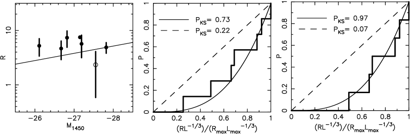
Figure 1: Correlations between the properties of the $z>6$ quasars and their H II regions. Left panel: correlation between quasar absolute magnitude (at rest-frame 1450Å)  $M_{1450}$ and inferred radius of the H II region around it $R$. The open circle shows the point for SDSS 1048+4637. The line corresponds to the naive expectation that $R\propto L^{1/3}$. Central panel: cumulative probability histogram for $\eta\equiv RL^{-1/3}/(RL^{-1/3})_{\rm max}$. The solid line corresponds to $P(<\eta)=\eta^{3}$, and the dashed line to a random distribution. Right panel: same as for the central panel, but with SDSS 1048+4637 omitted.

We now examine the correlation between the properties of the $z>6$ quasars and the sizes of their H II regions. The left hand panel of Figure 1 shows the correlation between the measured absolute magnitude at a rest-frame wavelength of $1450$Å, $M_{1450}$, and the inferred radius of the H II region, $R$. The line corresponds to the naive expectation that $R\propto L^{1/3}$ (normalized to the quasar with the largest value of $RL^{-1/3}$). Scatter would be expected around this line for physical reasons (e.g. owing to different quasar ages) in addition to measurement errors. However, comparison of this line with data points constitutes an important systematic check that the bubbles do not show any unexpected trend.

Since the volume within the H II region grows approximately linearly with time, the observed bubble sizes should follow a characteristic distribution. The central panel of Figure 1 shows a cumulative probability histogram for $\eta\equiv RL^{-1/3}$ (normalized to the quasar with the largest value of $RL^{-1/3}$ so that $0\leq\eta\leq 1$). For a random sample of quasar ages, this distribution would be expected to follow $P(<\eta)=\eta^{3}$ (solid line). The expected and measured curves are fully consistent in a Kolmogorov-Smirnov (KS) test with a probability $P_{\rm KS}\sim 0.7$. On the other hand if the observed size of the Ly$\alpha$ transmission region had been set by a dense absorbing cloud rather than by the neutral IGM, then we would expect a random distribution of bubble sizes $R$. Since $R$ and $L$ would be uncorrelated in this case, the distribution of $RL^{-1/3}$ would also be random. However we find that a random distribution (dashed line) is also consistent in a KS test, with $P_{\rm KS}\sim 0.2$.

We note one possible anomaly in the redshifts listed in Table 1. The object SDSS 1048+4637 is the only source with a value of $z_{\rm MgII}<z_{\rm Ly\alpha,CIV}$, which is not expected given the distribution of blueshifts for high ionization lines (Richards et al. 2002). SDSS 1048+4637 is also the only object with a value of $z_{\rm MgII}-z_{\rm GPT}$, and hence a size for the H II region that is consistent with zero (open circle in the left hand panel of Figure 1). One would need an observationally motivated reason to eliminate this quasar from the sample; nevertheless, it is interesting to repeat the above comparison of distributions in the absence of SDSS 1048+4637 (right hand panel of Figure 1). In this case we see that while the distribution is consistent with volumes of H II regions that grow linearly with time ($P_{\rm KS}\sim 0.9$), a random distribution is now only consistent with the data at the 7% level. In the future, using a larger sample of quasars (perhaps from the completed SDSS) we may be able to reject the random distribution. For now, we will return to the possibility that dense absorbing clouds might mimic the signature of H II regions in a neutral IGM in section 2.2.

Another possible source of systematic uncertainty arises from gravitational lensing. The large magnification bias for quasars on the bright end of the quasar luminosity function implies that strong gravitational lensing may be one or even two orders of magnitude more common in the SDSS $z\sim 6$ quasars than in lower redshift samples (Wyithe & Loeb 2002a;2002b; Commerford, Haiman & Schaye 2002). Undetected lensing leads to an overestimate of the quasar luminosity. In the present analysis this leads to an overestimate of the neutral fraction. Currently there is high resolution imaging for four of the $z>6$ quasars. As part of an HST snapshot survey of high redshift quasars, SDSS 1030+0524 and SDSS 1306+0356 have been imaged (Richards et al. 2003). In addition Keck K-band images have been obtained for SDSS 1048+4637 and SDSS 1148+5251 (Fan et al. 2003), while SDSS 1148+5251 has also been imaged with HST (White et al. 2004). None of these images show evidence for strong lensing, and hence for significant magnification (however see Keeton, Kuhlun & Haiman 2004). As a result we do not consider lensing in our analysis.

3 The model

The model used in this paper to compute the evolution of quasar H II regions has been previously described in Wyithe & Loeb (2004a). However for completeness we present a summary of its main features below.

Quasars are assumed to be powered during the hierarchical growth of their host galaxy. Bright episodes are triggered when halos merge. Within our model, we generate many random realizations of the merger tree of the host halo at $z=6.5$, assign super-massive black holes (SMBHs) to these halos and compute the time-dependent luminosity that is triggered during the merges. Each tree has $N_{\rm merge}$ major mergers, which occur at times $t_{j}$. We assume a relation between the black-hole and galaxy halo mass that preserves the correlation between the circular velocity of the halo and the black-hole mass it hosts in the form

$$M_{\rm halo}=1.5\times 10^{12}M_{\odot}\left(\frac{M_{\rm bh}}{10^{9}M_{\odot}}\right)^{3/5}\left(\frac{1+z}{7}\right)^{-3/2}.$$ (2)

Inferred black-hole masses for the SDSS quasars of $M_{\rm bh}\sim 10^{9}M_{\odot}$ imply halo masses of $M_{\rm halo}\sim 10^{12}M_{\odot}$ (Wyithe & Loeb 2003). Since this relation is non-linear, there is a mass differential between the coalesced black-hole mass and the mass of the new halo. We define a parameter $f_{\rm lt}\equiv f_{\rm mass}/\eta_{\rm Edd}$, where $f_{\rm mass}$ is the fraction of the mass differential that is accreted during the luminous phase and $\eta_{\rm Edd}$ is the fraction of the Eddington rate at which the mass is accreted. If a merger of two halos leads to coalescence of their black-holes, and the mass differential is accreted during a luminous phase over which the quasar shines near its Eddington limiting luminosity, then the quasar lifetime is

$$t_{\rm lt}=f_{\rm lt}\times 4\times 10^{7}\left(\frac{\epsilon}{0.1}\right)\ln\left[\frac{\left(M_{1}+M_{2}\right)^{5/3}}{M_{1}^{5/3}+M_{2}^{5/3}}\right]\hskip 5.69054pt\mbox{years},$$ (3)

where $M_{1}$ and $M_{2}$ are the masses of the merging halos, and $\epsilon$ (taken to be 0.1) is the radiative efficiency. Note that the lifetime increases for sub-Eddington accretion. The parameter $f_{\rm lt}$ may be thought of as the fraction of our fiducial lifetime during which the quasars shine, leading to quasar lifetimes of $t_{\rm lt}\sim f_{\rm lt}\times 10^{7}$ years. The model lifetime is therefore consistent with current estimates [$10^{6}-10^{8}$ years; see Martini (2003) for a summary] for values of $f_{\rm lt}$ that are of order unity. We assume that each quasar episode $j$ has an exponential light-curve

$$\dot{N}_{j}(t)=\Theta\left(t-t_{j}\right)\dot{N}_{0,j}\exp{\{-(t-t_{j})/t_{\rm lt}\}}$$ (4)

beginning at $t_{j}$ and with a characteristic decay time of $t_{\rm lt}$ during which the SMBH shines at its Eddington luminosity, $L_{E}=1.4\times 10^{47}~{}{\rm erg~{}s^{-1}}(M_{\rm bh}/10^{9}M_{\odot})$. Here $\Theta$ is the Heaviside step function. The time dependent ionizing luminosity within the merger tree is then computed from the sum of luminous episodes $\dot{N}(t)=\sum_{j=1}^{N_{\rm merge}}\dot{N}_{j}$. Following Telfer et al. (2002) and White et al. (2003), we adopt an ionizing photon emission rate of $\dot{N}_{0,j}=2\times 10^{57}$s${}^{-1}/\left({\alpha_{{\rm EUV},j}}/{-1.75}\right)$, where $\alpha_{{\rm EUV},j}$ is the spectral index in the EUV band during the $j$th merger. Telfer et al. (2002) find $\alpha_{\rm EUV}=-1.75\pm 0.75$, and we assign a value of $\alpha_{{\rm EUV},j}$ to each merger in the tree from a normal distribution of mean -1.75 and standard deviation 0.75.

The evolution of the physical radius of the H II region, $R$, may then be found through integration of the differential equation

$$\frac{dR}{dt}=c\left[\frac{F_{\gamma}\dot{N}(t)-\alpha_{\rm B}CF_{\rm m}x_{\rm HI}\left(\bar{n}_{0}^{\rm H}\right)^{2}\left({4\pi\over 3}R^{3}\right)}{F_{\gamma}\dot{N}(t)+4\pi R^{2}\left(1+z\right)^{-1}cF_{\rm m}x_{\rm HI}\bar{n}_{0}^{\rm H}}\right],$$ (5)

where $c$ is the speed of light, $\bar{n}_{0}^{\rm H}$ is the mean number density of protons at $z=0$, $\alpha_{\rm B}=2.6\times 10^{-13}$cm³s^-1 is the case-B recombination coefficient at the characteristic temperature of $10^{4}$K, and $\dot{N}_{\rm ion}$ is the rate of ionizing photons crossing a shell at the radius of the H II region at time $t$. We use the distribution derived from numerical simulations for the over-densities $\Delta$ in gas clumps (Miralda-Escude, Haehnelt & Rees 1998), and calculate the mean free path for ionizing photons $d(\Delta_{\rm c})$ as a function of the critical overdensity $\Delta_{\rm c}$ (Miralda-Escude, Haehnelt & Rees 1998; Barkana & Loeb 2002). Following Barkana & Loeb (2002), we then find the value of $\Delta_{\rm c}$ at which a fraction $\exp\left[-R/d(\Delta_{\rm c})\right]=50\%$, of the emitted photons do not encounter an overdensity larger than $\Delta_{\rm c}$ within the H II region. We also compute the mass fraction $F_{\rm m}$ ($\sim 1$) of gas within $R$ that is at over-densities lower than $\Delta_{\rm c}$. Finally, we calculate the clumping factor in the ionized regions, $C(R)\equiv\langle\Delta^{2}\rangle/\langle\Delta\rangle^{2}$, where the angular brackets denote an average over all regions with $\Delta<\Delta_{\rm c}$. For $x_{\rm HI}=1$ and $dR/dt\ll c$, equation (5) reduces to its well-known form (e.g. Madau & Rees 2001). The emission rate of ionizing photons $\dot{N}$ in equation (5) is computed at $t^{\prime}=t-t_{\rm delay}$ to account for the finite light travel time between the source and the ionization front.

Note that while equation (5) is expressed in terms of the radius of a spherical H II region, there is no implicit assumption about isotropy in the analysis presented in this paper. This is because both the volume of the HII region and the luminosity of the quasar are measured per unit solid angle along the line-of sight. The extrapolations to total volume and total luminosity are made by multiplying these quantities by $4\pi$ purely for convenience of presentation.

In our calculation we require that the quasar ionize regions up to a sufficiently high overdensity, so as to allow the ionizing photon mean-free-path to exceed the radius of the H II region. The highest density regions (which are sufficiently compact to allow a long mean-free-path) may remain neutral. The value of $x_{\rm HI}$ in equation (5) refers to the neutral fraction in the low density regions. We therefore interpret the neutral fraction $x_{\rm HI}$ in equation (5) as volume weighted rather than mass weighted fraction.

In the hierarchical picture of structure formation, the appearance of the quasar and the surrounding galaxies will occur concurrently. The neutral fraction into which the quasar H II region expands therefore reflects the contribution to reionization due to stellar flux from the quasar host and surrounding galaxies (see Fig. 2 in Wyithe & Loeb 2004c for their relative significance). As the quasar and stellar ionizing fluxes are emitted at the same cosmic epoch, we implicitly assume that both are responsible for reionizing the low density regions, such that both have an ionizing photon mean free path that exceeds the radius of the H II region. In this our model differs markedly from the work described in Yu & Lu (2004), where quasar flux is assumed to be emitted into an IGM whose low density regions have already been ionized by stars at some prior epoch. In that work the clumping factor associated with quasar ionizing flux is evaluated above the density threshold corresponding to a mean-free-path that equals the size of the H II region, i.e. it is assumed that stars ionize the low density regions while the quasar ionizes only the high density regions. As a result, Yu & Lu (2004) infer a much higher clumping factor than we find here, and conclude in difference to this work that the quasar flux does not provide a significant contribution to the growth of the H II regions.

Several consequences of our simple model can be immediately confronted with observational data. Evidence from direct determination of the $M_{\rm bh}$–velocity dispersion relation (Shields et al. 2003), as well as the redshift evolution of the quasar correlation function (Wyithe & Loeb 2004b), suggest that the assumed relation (equation 2) is indeed preserved out to a redshift of at least $z\sim 3$. Preliminary support for an extrapolation of the relation out to $z\sim 6$ comes from the velocity shift of the Ly$\alpha$ absorption feature due to the galactic virialization shock, whose amplitude gauges the circular velocity and hence mass of the host halo for some high-redshift quasars (Barkana & Loeb 2003). The presence of a massive galaxy is also implied by the molecular mass of $>10^{10}M_{\odot}$ in the host galaxy of SDSS1148$+$5251 (Walter et al. 2003; 2004) and the velocity width of $280~{}{\rm km~{}s^{-1}}$ for its CO lines (Bertoldi et al. 2003). The measured CO velocity width corresponds to a dark halo mass of $\sim 10^{11}M_{\odot}$ at $z=6.4$, which is insufficient to contain the inferred molecular gas mass. Indeed, $280$km s^-1 is much smaller than the $\sim 500$km s^-1 we would expect to be associated with a SMBH of $\sim 10^{9}M_{\odot}$ (Wyithe & Loeb 2003,2004b), which is thought to power the observed quasar. A possible explanation for this inconsistency is that the CO observations only sample the gravitational potential within a few kpc from the galaxy center while the galaxy halo has a much deeper potential well. To quantify this uncertainty we note that the number of major mergers per logarithm of mass increases by a factor of $\sim 2.4$ if the host dark matter halo mass for the SDSS quasars is an order of magnitude smaller than assumed (i.e. $10^{11}M_{\odot}$ rather than $10^{12}M_{\odot}$). Thus, adopting a smaller dark matter halo at the bottom of the merger tree would lead to a higher merger rate, a more frequent quasar activity, and hence the inference of a larger neutral fraction.

Additional support for the assumed $M_{\rm halo}-M_{\rm bh}$ relation comes from attempts to model the luminosity function of quasars using the abundance of halos and the $M_{\rm bh}-\sigma$ relation (Volenteri, Haardt & Madau 2002; Wyithe & Loeb 2003). These models are equally successful at $z\sim 6$ as they are at lower redshifts $z\sim 2$–$3$ where data exists on the $M_{\rm bh}-\sigma$ relation. These physically motivated models for the luminosity function also suggest a quasar lifetime that is in the vicinity of $10^{6}-10^{7}$ years at $z\sim 6$. Comparing with $t_{\rm lt}$ (as calculated from equation 3) implies a value $f_{\rm lt}>0.1$, or in other words that most of the SMBH mass at $z>6$ was accreted during the luminous phase. Indeed having all the black-hole mass accreted during the luminous phase ($f_{\rm lt}=1$) is consistent with the census of mass in local dormant SMBHs, compared with the mass accreted during luminous quasar phases throughout the history of the universe. These studies are most sensitive to conditions at $z\sim 2-3$, but find the majority of SMBH mass to have been accreted during luminous quasar phases near the Eddington limit, and with a radiative efficiency of $\epsilon\sim 0.1$ (Yu & Tremaine 2002).

To estimate the ionizing luminosity of the $z>6$ quasars we use the median spectrum of low redshift quasars derived by Telfer et al. (2002), scaled to the appropriate luminosity of the quasar ($M_{1450}$). The assumption of no evolution of the quasar spectrum over 90% of the age of the universe is supported by the observation that the median rest frame UV spectrum of the high redshift quasars is consistent with that at low redshift (Fan et al. 2004). In addition, the recently observed X-ray spectrum of SDSS 1306+0356 implies an optical to X-ray spectral index that is consistent with radio-quiet quasars at lower redshift (Schwartz & Virani 2004). These results imply little evolution in quasar spectra, and justify our use of the low redshift median quasar spectrum for the analysis of the $z>6$ quasars.

Figure 2: Cumulative probability for the neutral fraction of the IGM, $x_{\rm HI}$. The thin lines show the distributions for individual quasars, while the thick line shows the combined result. Left: $f_{\rm lt}=0.1$. Right: $f_{\rm lt}=1$.

4 Constraints on the Neutral Fraction

Next we derive limits on the neutral fraction of hydrogen surrounding the $z>6$ quasars. Our basic method follows that outlined in Wyithe & Loeb (2004a). However we have augmented the approach to reflect the richer data set now available.

Figure 3: Limits from individual quasars as a function of their redshift. Each quasar is represented by a point. From bottom up, the curves show the 1st, 10th, 90th and 99th percentiles of $P(<x_{\rm HI})$. The left and right-hand panels show the cases of $f_{\rm lt}=0.1$ and $f_{\rm lt}=1$, respectively, and limits derived from SDSS 1048+4637 are denoted by an open circle. The dotted curves provide the integral of a normal distribution in redshift $\int_{0}^{z}dz^{\prime}N(6.4,0.15)$.

We compute the conditional probability distributions $\left.\frac{dP_{i}}{dR}\right|_{x_{\rm HI}}$ for the observed radius of the H II region surrounding each quasar as a function of the neutral fraction of hydrogen, $x_{\rm HI}$. Based on these distributions we find the likelihood for the neutral fraction from the observed radius around each quasar

$$L_{i}(x_{\rm HI})=\int dR_{i}N(\bar{R}^{\rm obs}_{i},\sigma_{\rm R_{i}})\left.\frac{dP_{i}}{dR}\right|_{x_{\rm HI}}(R=R_{i})$$

Here $N(x,\sigma_{x})$ is a normal distribution of mean $x$ and variance $\sigma_{x}$. The values of mean and variance of the radii are given in Table 1. Assuming the neutral fraction to have the same value around all quasars in the sample, we also find the joint likelihood

$$L(x_{\rm HI})=\Pi_{i=1,7}L_{i}.$$ (6)

The relative likelihood for $x_{\rm HI}$ may be combined with its a-priori probability distribution $dP_{\rm prior}/dx_{\rm HI}$ to yield cumulative a-posteriori probability distributions

$$P_{i}(<x_{\rm HI})=N_{i}\int_{0}^{x_{\rm HI}}dx^{\prime}_{\rm HI}L_{i}(x^{\prime}_{\rm HI})\frac{dP_{\rm prior}}{dx^{\prime}_{\rm HI}},$$ (7)

and

$$P(<x_{\rm HI})=N\int_{0}^{x_{\rm HI}}dx^{\prime}_{\rm HI}L(x^{\prime}_{\rm HI})\frac{dP_{\rm prior}}{dx^{\prime}_{\rm HI}},$$ (8)

where $N$ and $N_{i}$ are normalizing constants such that $P_{i}(<1)=1$ and $P(<1)=1$ respectively. In this paper we adopt a logarithmic prior for $x_{\rm HI}$, i.e. $dP_{\rm prior}/dx_{\rm HI}\propto 1/x_{\rm HI}$ for $10^{-3}<x_{\rm HI}<1$, corresponding to the range allowed by observations of the GP trough (White et al. 2003). More stringent limits are found for $x_{\rm HI}$ if a flat prior is assumed.

In Figure 2 we plot the cumulative probability of $x_{\rm HI}$. The thin lines show the distributions for individual quasars, whereas the thick line shows the combined result. The left panel shows the case of $f_{\rm lt}=0.1$, corresponding to the situation where the quasar fiducial lifetime in equation (3) overestimates the true lifetime by a factor of 10. The right hand panel shows the fiducial case, with $f_{\rm lt}=1$. We note that each of the seven quasars individually yields a consistent result that $x_{\rm HI}$ is of order 0.1–1. The combined constraint shown by the thick line is therefore not controlled by observations of just one or a couple of the quasar H II regions. The combined constraint for the fiducial model is $x_{\rm HI}>0.1$ ($f_{\rm lt}=0.1$) and $x_{\rm HI}>0.7$ ($f_{\rm lt}=1$) at the 90% confidence level. Clearly $f_{\rm lt}$ is a limiting systematic uncertainty and we return to its dependence below.

In Figure 3 we examine the dependence of the individual quasar limits on the quasar redshift. Each quasar is represented by 4 points (with SDSS 1048+4637 denoted by open circles), which from bottom up show the 1st, 10th, 90th and 99th percentiles of $P_{i}(<x_{\rm HI})$. Lines join these points for each percentile to guide the eye. The left and right-hand panels illustrate the cases of $f_{\rm lt}=0.1$ and $f_{\rm lt}=1$, respectively. The apparent trend is that higher limits on $x_{\rm HI}$ are derived for higher redshift quasars. This trend is to be expected if the quasars are observed near the end of the reionization process.

The variation of constraints with quasar redshift may be compared with expectations from theory. The redshift at which a region of a given size is reionized is proportional to the linear overdensity on that scale (Barkana & Loeb 2003). Along different lines of sight this redshift has a Gaussian distribution with a variance given by the power spectrum of primordial fluctuations. Wyithe & Loeb (2004d) have shown that the combined constraints of finite light travel time and cosmic variance imply that the scatter in the redshift at which neutral IGM would be encountered along a random line of sight is $\Delta z\sim 0.15$. This scatter defines a minimum rate over which the IGM could become reionized. For comparison with the observed limits, the dashed line in Figure 3 therefore shows the cumulative distribution corresponding to a Gaussian with variance $0.15$ around a central redshift of 6.4 (which results in a neutral fraction of $x_{\rm HI}\sim 10^{-3}$ at $z\sim 5.85$ where limits exist based on the optical depth in the GP trough). The limits from individual quasars imply a somewhat slower evolution in the neutral fraction than the maximum rate described by the dashed curve, as expected.

As already mentioned, the largest systematic uncertainty in the analysis described is the value of $f_{\rm lt}$. While we expect $f_{\rm lt}\sim 1$, it is instructive to compute the limits on the neutral fraction as a function of $f_{\rm lt}$. In Figure 4 we show the 1st, 10th, 90th and 99th percentiles of $P(<x_{\rm HI})$ from the bottom up. Smaller values of $f_{\rm lt}$ yield less stringent limits. However we find that $x_{\rm HI}>0.1$ for all $f_{\rm lt}>0.1$, and $x_{\rm HI}>0.01$ for all $f_{\rm lt}>0.025$ at 90% confidence. These limits represent a significant improvement upon the limits for the volume averaged neutral fraction based on the optical depth in the GP trough, $x_{\rm HI}>10^{-3}$ (White et al. 2003).

Figure 4: The neutral fraction as a function of $f_{\rm lt}$. From the bottom up, the lines show the 1st, 10th, 90th and 99th percentiles of $P(<x_{\rm HI})$ respectively.

5 Conclusion

In this paper we have extended an earlier analysis of the neutral fraction of hydrogen in the IGM around SDSS 1148+5251 and SDSS 1030+0524 (Wyithe & Loeb 2004a) to include all seven quasars now known at $z\gtrsim 6$. We have used updated redshifts for the hosts of these quasars and incorporated uncertainties in the measured size of their H II region. The small size of the H II regions implies that the typical neutral hydrogen fraction of the IGM beyond $z\sim 6$ is in the range 0.1–1. This result also holds for the IGM surrounding each individual quasar when the H II regions are considered separately. The primary systematic uncertainty in the analysis is the quasar lifetime. However by combining the limits for the six quasars, we find that at the 99% level, the neutral fraction is larger than 0.08 for quasar lifetimes $>10^{6}$ years, or larger than 0.6 for lifetimes $>10^{7}$ years. These lifetimes correspond to only $10^{-3}$ and $10^{-2}$ Hubble times respectively at $z\sim 6$ and are favored by empirical constraints on the lifetime of lower-redshift quasars (e.g. Martini 2003). Larger duty-cycles lead to stronger limits. We find that the size distribution of H II regions is consistent with the expected distribution for observations that are made randomly in time. In addition, we find that constraints on the neutral fraction obtained from individual quasars are stronger at higher redshift. This is to be expected if the universe is nearing the end of reionization at $z\sim 6$ as the neutral fraction drops with time. A larger sample of quasar H II regions from the full SDSS, or those discovered by forthcoming redshifted 21cm surveys (Wyithe & Loeb 2004e) will allow more stringent checks of these trends.

References

- (1) Barkana, R., Loeb, A. 2001, Phys. Rep., 349, 125
- (2) ———————. 2002, ApJ, 578, 1
- (3) ———————. 2003, Nature, 421, 341
- (4) ———————. 2004, ApJ, 601, 64
- (5) Bertoldi, F., et al., 2003, Astron. Astrophys, Lett., 409, L47
- (6) Cen, R. 2003, ApJ, 591, L5
- (7) Cen, R., Haiman, Z., 200, ApJ, 542, L74
- Comerford, Haiman, & Schaye (2002) Comerford, J. M., Haiman, Z., & Schaye, J. 2002, ApJ, 580, 63
- (9) Fan, X., et al. 2001 AJ, 122, 2833
- (10) ——————–. 2003, astro-ph/0301135
- (11) ——————–. 2004, AJ, in press; astro-ph/0405138
- (12) Furlanetto, S.R. , Hernquist, L. & Zaldarriaga, M. 2004, MNRAS, submitted, astro-ph/0406131
- (13) Freudling W., Corbin, M.R., Korista, K.T., 2003, ApJ, 587, L67
- (14) Gnedin, N.Y., Prada, F. 2004, ApJ, 608, L77
- (15) Gunn, J. E. & Peterson, B. A. 1965, ApJ, 142, 1633
- (16) Iwamuro et al. 2004, astroph/0408517
- (17) Keeton, C., Kuhlun, M. Haiman, Z., 2004, astro-ph/0405143
- (18) Kogut, A. et al. 2003, ApJ, submitted; astro-ph/0302213
- (19) Madau, P., Rees, M.J., 2000, ApJ, 542, L69
- (20) Maiolino et al. 2003, astroph/0312402
- Miralda-Escudé, Haehnelt, & Rees (2000) Miralda-Escudé, J., Haehnelt, M., & Rees, M. J. 2000, ApJ, 530, 1
- (22) Martini, P. 2003, to appear in ”Carnegie Observatories Astrophysics Series, Vol. 1: Coevolution of Black Holes and Galaxies,” ed. L. C. Ho (Cambridge: Cambridge Univ. Press); astro-ph/0304009
- (23) Mesinger, A. & Haiman, Z. 2004, ApJ, submitted; astro-ph/0406188
- (24) Miralda-Escude, J. 2003, ApJ, 597, 66
- (25) Oh, S.P., Furlanetto, S.R., 2004, ApJL, submitted, astro-ph/0411152
- (26) Rhoads, J.E., et al., ApJ, in press, astro-ph/0403161
- (27) Richards, G.T., et al., 2002, Astron. J. Supp., 124, 1
- (28) ——————–. 2003, Astron.J., 127, 1305
- Schirber & Bullock (2003) Schirber, M. & Bullock, J. S. 2003, ApJ, 584, 110
- (30) Schwartz, D. A., & Virani, S. N. 2004, preprint, astro-ph/0410124
- (31) Shields, G.A., et al. 2003, ApJ 583, 124
- (32) Spergel, D. N, et al. 2003, AJ Supp., 148, 175
- (33) Storrie-Lombardi, L. J. & Wolfe, A. M. 2000, ApJ, 543, 552; Erratum-ibid. 592, 1263
- (34) Telfer, R. C., Zheng, W., Kriss, G. A., Davidsen, A. F. 2002, AJ, 565, 773
- Tytler & Fan (1992) Tytler, D. & Fan, X. 1992, ApJS, 79, 1
- (36) Volonteri, M., Haardt, F., Madau, P., 2003, ApJ, 582, 559
- (37) Walter, F., et al., 2003, Nature, 424, 406
- (38) Walter, F., Carilli, C., Bertoldi, F., Menten, K., Cox, P., Lo, K.Y., Fan, X., Strauss, M., 2004, ApJL, accepted, astro-ph/0410229
- (39) White, R., Becker, R., Fan, X., Strauss, M. 2003, AJ, 126, 1
- (40) White, R., Becker, R., Fan, X., Strauss, M. 2004, astro-ph/0411195
- Willott, McLure, & Jarvis (2003) Willott, C. J., McLure, R. J., & Jarvis, M. J. 2003, astro-ph/0303062
- Wyithe & Loeb (2002) Wyithe, J. S. B. & Loeb, A. 2002a, Nature, 417, 923
- Wyithe & Loeb (2002) ——————–. 2002b, ApJ, 577, 57
- (44) ——————–. 2003a, ApJ, 588, 69
- (45) ——————–. 2003b, ApJ 595, 614
- (46) ——————–. 2004a, Nature, 427, 815
- (47) ——————–. 2004b, ApJ, accepted, astro-ph/0403614
- (48) ——————–. 2004c, ApJ, submitted, astro-ph/0407162
- (49) ——————–. 2004d, Nature, in press, astro-ph/0409412
- (50) ——————–. 2004e, ApJ, accepted, astro-ph/0401554
- (51) Yu, Q., Tremaine, S., 2002, MNRAS, 335, 965
- (52) Yu, Q., Lu, Y., 2004, ApJ., accepted, astro-ph/0411098