Rosseland and Planck mean opacities for primordial matter

Abstract

We present newly calculated low-temperature opacities for gas with a primordial chemical composition. In contrast to earlier calculations which took a pure metal-free Hydrogen/Helium mixture, we take into account the small fractions of Deuterium and Lithium as resulting from Standard Big Bang Nucleosynthesis. Our opacity tables cover the density range $-16<\log\rho\hskip 2.84544pt[\textup{g}\textup{ cm}^{-3}]<-2$ and temperature range of $1.8<\log T\hskip 2.84544pt[\textup{K}]<4.6$, while previous tables were usually restricted to $T>10^{3}\,\mathrm{K}$. We find that, while the presence of Deuterium does not significantly alter the opacity values, the presence of Lithium gives rise to major modifications of the opacities, at some points increasing it by approximately 2 orders of magnitude relative to pure Hydrogen/Helium opacities.

1 Introduction

According to the Standard Big Bang Nucleosynthesis (SBBN), the most abundant elements in the aftermath of the Big Bang were Hydrogen and Helium with very small traces of Deuterium and Lithium. These elements make up the so called POP iii or primordial chemical composition. All the heavier elements present today had to be produced in the course of the evolution of several generations of stars.

In order to understand the physics of the early Universe, there is a need of having appropriate and accurate material functions at hand, in particular opacities for a SBBN chemical compositions.

There is a large body of literature available with opacity calculations for metal-free (Z=0) H/He mixtures, starting with the Paczynski I-VI mixtures (Cox & Tabor, 1976, hereafter CT76), the calculations of Stahler et al. (1986, hereafter SPS86) and Lenzuni et al. (1991, hereafter LCS91), and more recently Harris et al. (2004, hereafter HLMT04).

These calculations were restricted to temperatures between $10^{3}\textup{ K}$ and $10^{4}\textup{ K}$. Specific metal-free opacity sets have been calculated by the OP project (Seaton et al., 1994, $10^{3.75}\dots 10^{8}\textup{ K}$) and OPAL (Alexander & Ferguson, 1994; Iglesias & Rogers, 1996, $10^{3}\dots 10^{8.7}\textup{ K}$). More recently, OPAL calculations have been extended (Eldridge & Tout, 2004) to $10^{3}\dots 10^{10}\textup{ K}$ and densities $-8<\log\textup{ R}<7$ with the main application for CNO enhanced opacities in stellar evolution.

All these opacity calculations, however, only considered pure Hydrogen/Helium mixtures with no metals (mass fraction $Z=0$), but different ratios $X/Y$ of the mass fractions of Hydrogen ($X$) and Helium ($Y$). It has been argued that due to the assumed very small abundances of Deuterium and Lithium these element do not play any significant role in the opacities and thus in the evolution of POP iii objects.

Moreover, while there are good low-temperature opacities available for a solar chemical composition (e.g. Semenov et al., 2003), zero-metallicity opacity tabulations have been restricted to temperatures above $1000\textup{ K}$ so far.

In this paper we present calculations of both, Rosseland and Planck mean opacities for primordial matter including all the three elements (Hydrogen, Helium, and Lithium) including Deuterium isotope and present their absorption properties.

In Sect. 2 we discuss the quantitative composition of primordial matter at a given temperature and density. We then describe the relevant absorption processes (Sect. 3) and present our Rosseland and Planck mean opacities (Sect. 4). Here, we also assess the influence of Lithium on the opacity for different Lithium contents. Before we compare our results to previous tabulations (Sect. 6), we give analytic calculations for the molecule formation timescale in Sect. 5 in order to estimate the time needed to reach chemical equilibrium which is one of the underlying assumptions in our calculations. Finally, we summarize our conclusions in Sect. 7.

2 Primordial Matter

Primordial Matter as created in the SBBN consists of Hydrogen (H), Helium (He), Deuterium (D), and Lithium (Li). Before WMAP(Spergel et al., 2003), the observed abundances of these elements have been used to constrain the baryon-to-photon ratio. In the framework of a $\Lambda$CDM cosmology WMAP provided the value this parameter with high accuracy. While the abundances of H and He were fairly well known for some time, the uncertainties in the determination of the abundances of D and Li were significantly reduced. Now, the D abundance as derived from cosmological parameters is consistent with direct observations, while the observed Li abundance still lacks a factor of 3 compared to the SBBN results. This may indicate either systematic effects in the observations or new physics (for an in-depth discussion of this issue, see Coc et al., 2004). We summarize the resultant abundances according to SBBN and WMAP in Table 1 (after Coc et al., 2004) and take them as our fiducial POP iii mixture. For later comparison purposes we define also a Li-free mixture in Table 1.

	POP III	Li-free
Y	$(0.2479\pm 0.0004)$	$(0.2479\pm 0.0004)$
D/H	$(2.60^{+0.19}_{-0.17})\cdot 10^{-5}$	$(2.60^{+0.19}_{-0.17})\cdot 10^{-5}$
${}^{3}\textup{He}/\textup{H}$	$(1.04^{+0.04}_{-0.04})\cdot 10^{-5}$	$(1.04^{+0.04}_{-0.04})\cdot 10^{-5}$
${}^{7}\textup{Li}/\textup{H}$	$(4.15^{+0.49}_{-0.45})\cdot 10^{-10}$	$0$

Table 1: SBBN concordance abundances (Coc et al., 2004) from first-year WMAP results

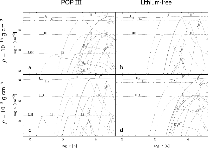
Figure 1: The influence of the presence or absence of Li on the EOS for two densities: (a) $\rho=10^{-13}\textup{ g}\textup{ cm}^{-3}$, POP iii; (b) $\rho=10^{-13}\textup{ g}\textup{ cm}^{-3}$, Li-free; (c) $\rho=10^{-5}\textup{ g}\textup{ cm}^{-3}$, POP iii; (d) $\rho=10^{-5}\textup{ g}\textup{ cm}^{-3}$, Li-free. The different lines have the following meanings: solid red line – electron abundance; dotted blue lines – abundance of neutral molecules; dashed purble lines – positive ions; dash-dotted black lines – negative ions; dash-triple-dotted green lines – abundance of neutral atoms.

2.1 Equation of state (EOS)

We consider 20 species of primordial matter: electrons $\textup{e}^{-}$, Hydrogen species $\textup{H}^{-}$, H, $\textup{H}^{+}$, $\textup{H}_{2}$, $\textup{H}_{2}^{+}$, and $\textup{H}_{3}^{+}$, Helium species He, $\textup{He}^{+}$, $\textup{He}^{++}$, and $\textup{He}_{2}^{+}$, Deuterium species D, $\textup{D}^{+}$, HD, and $\textup{H}_{2}\textup{D}^{+}$, and Lithium species Li, $\textup{Li}^{+}$, $\textup{Li}^{++}$, LiH and $\textup{LiH}^{+}$.

The computations assume chemical and thermodynamical equilibrium. Equilibrium constants (see Table 2) are used whenever they are available in the literature, otherwise appropriate Saha equations are taken.

For the partition functions the most recent $\textup{H}_{3}^{+}$ partition function $Q_{\textup{H}_{3}^{+}}$ of Neale & Tennyson (1995), for $\textup{H}_{2}^{+}$ Stancil (1994a) is used. For HD and $\textup{H}_{2}$ a partition function for the equilibrium constant is calculated using the energy levels for HD (Stancil & Dalgarno, 1997) and $\textup{H}_{2}$ . All other partition functions needed for the Saha equations are approximated by the ground state statistical weight.

Combining all the equilibrium constants, there are 5 equations utilizing mass conservation of all 4 elements and charge neutrality. These equations are solved using an iterative procedure (see Appendix A).

$\textup{H}_{2}\leftrightarrow\textup{H}+\textup{H}$	$K_{\textup{H}_{2}}=\frac{{\left[\textup{H}\right]}{\left[\textup{H}\right]}}{{\left[\textup{H}_{2}\right]}}$	Saha $(U=4.478\textup{ eV})$
$\textup{H}^{-}\leftrightarrow\textup{H}+\textup{e}^{-}$	$K_{\textup{H}^{-}}=\frac{{\left[\textup{H}\right]}[\textup{e}^{-}]}{{\left[\textup{H}^{-}\right]}}$	Saha $(U=0.7556\textup{ eV})$
$\textup{H}\leftrightarrow\textup{H}^{+}+\textup{e}^{-}$	$K_{\textup{H}}=\frac{{\left[\textup{H}^{+}\right]}{\left[\textup{e}^{-}\right]}}{{\left[\textup{H}\right]}}$	Saha $(U=13.6\textup{ eV})$
$\textup{H}_{2}^{+}\leftrightarrow\textup{H}+\textup{H}^{+}$	$K_{\textup{H}_{2}^{+}}=\frac{{\left[\textup{H}\right]}{\left[\textup{H}^{+}\right]}}{{\left[\textup{H}_{2}^{+}\right]}}$	Stancil (1994a)
		$D_{0}=2.6507\textup{ eV}$ (Huber & Herzberg, 1979)
$\textup{H}_{2}^{+}+\textup{H}_{2}\leftrightarrow\textup{H}_{3}^{+}+\textup{H}$	$K_{\textup{H}_{3}^{+}}=\frac{{\left[\textup{H}_{3}^{+}\right]}{\left[\textup{H}\right]}}{{\left[\textup{H}_{2}^{+}\right]}{\left[\textup{H}_{2}\right]}}$	see App. C ($D_{0}=0.7382\textup{ eV}$, Sidhu et al., 1992)
$\textup{HD}\leftrightarrow\textup{H}+\textup{D}$	$K_{\textup{HD}}=\frac{{\left[\textup{H}\right]}{\left[\textup{D}\right]}}{{\left[\textup{HD}\right]}}$	Saha ($U=4.5167\textup{ eV}$, Stancil & Dalgarno, 1997)
$\textup{D}\leftrightarrow\textup{D}^{+}+\textup{e}^{-}$	$K_{\textup{D}}=\frac{{\left[\textup{D}^{+}\right]}{\left[\textup{e}^{-}\right]}}{{\left[\textup{D}\right]}}$	$K_{\textup{D}}=K_{\textup{H}}$ (ass.)
$\textup{H}_{3}^{+}+\textup{D}\leftrightarrow\textup{H}_{2}\textup{D}^{+}+\textup{H}$	$K_{\textup{H}_{3}^{+},\textup{D}}=\frac{{\left[\textup{H}_{2}\textup{D}^{+}\right]}{\left[\textup{H}\right]}}{{\left[\textup{H}_{3}^{+}\right]}{\left[\textup{D}\right]}}$	Sidhu et al. (1992), $D_{0}=0.0439\textup{ eV}$
$\textup{H}_{3}^{+}+\textup{HD}\leftrightarrow\textup{H}_{2}\textup{D}^{+}+\textup{H}_{2}$	$K_{\textup{H}_{3}^{+},\textup{HD}}=\frac{{\left[\textup{H}_{2}\textup{D}^{+}\right]}{\left[\textup{H}_{2}\right]}}{{\left[\textup{H}_{3}^{+}\right]}{\left[\textup{HD}\right]}}$	Sidhu et al. (1992), $D_{0}=0.0120\textup{ eV}$
$\textup{He}\leftrightarrow\textup{He}^{+}+\textup{e}^{-}$	$K_{\textup{He}}=\frac{{\left[\textup{He}^{+}\right]}{\left[\textup{e}^{-}\right]}}{{\left[\textup{He}\right]}}$	Saha $(U=24.587\textup{ eV})$
$\textup{He}^{+}\leftrightarrow\textup{He}^{++}+\textup{e}^{-}$	$K_{\textup{He}^{+}}=\frac{{\left[\textup{He}^{++}\right]}{\left[\textup{e}^{-}\right]}}{{\left[\textup{He}^{+}\right]}}$	Saha $(U=54.418\textup{ eV})$
$\textup{He}_{2}^{+}\leftrightarrow\textup{He}+\textup{He}^{+}$	$K_{\textup{He}_{2}^{+}}=\frac{{\left[\textup{He}\right]}{\left[\textup{He}^{+}\right]}}{{\left[He_{2}^{+}\right]}}$	Stancil (1994a)
		$D_{0}=2.365\textup{ eV}$ (Huber & Herzberg, 1979)
$\textup{Li}\leftrightarrow\textup{Li}^{+}+\textup{e}^{-}$	$K_{\textup{Li}}=\frac{{\left[\textup{Li}^{+}\right]}{\left[\textup{e}^{-}\right]}}{{\left[\textup{Li}\right]}}$	$K_{\textup{Li}}=K_{\textup{LiH}^{+},1}\cdot\left.K_{\textup{LiH},2}\right/K_{\textup{LiH},1}$
$\textup{Li}^{+}\leftrightarrow\textup{Li}^{++}+\textup{e}^{-}$	$K_{\textup{Li}^{+}}=\frac{{\left[\textup{Li}^{++}\right]}{\left[\textup{e}^{-}\right]}}{{\left[\textup{Li}^{+}\right]}}$	Saha $(U=75.640\textup{ eV})$
$\textup{LiH}\leftrightarrow\textup{Li}+\textup{H}$	$K_{\textup{LiH},1}=\frac{{\left[\textup{Li}\right]}{\left[\textup{H}\right]}}{{\left[\textup{LiH}\right]}}$	Stancil (1996)
$\textup{LiH}\leftrightarrow\textup{LiH}^{+}+\textup{e}^{-}$	$K_{\textup{LiH},2}=\frac{{\left[\textup{LiH}^{+}\right]}{\left[\textup{e}^{-}\right]}}{{\left[\textup{LiH}\right]}}$	Stancil (1996)
$\textup{LiH}^{+}\leftrightarrow\textup{Li}^{+}+\textup{H}$	$K_{\textup{LiH}^{+},1}=\frac{{\left[\textup{Li}^{+}\right]}{\left[\textup{H}\right]}}{{\left[\textup{LiH}^{+}\right]}}$	Stancil (1996)
$\textup{LiH}^{+}\leftrightarrow\textup{Li}+\textup{H}^{+}$	$K_{\textup{LiH}^{+},2}=\frac{{\left[\textup{Li}\right]}{\left[\textup{H}^{+}\right]}}{{\left[\textup{LiH}^{+}\right]}}$	Stancil (1996)

Table 2: Equilibrium constants

2.2 Equilibrium $\textup{H}_{2}^{+}+\textup{H}_{2}\leftrightarrow\textup{H}_{3}^{+}+\textup{H}$

Since the early work of Patch (1968) it has been clear that $\textup{H}_{3}^{+}$ is important for temperatures of $2000-5000\,\mathrm{K}$ (Tennyson & Sutcliffe, 1984; Chandra et al., 1991; Sidhu et al., 1992; Neale & Tennyson, 1995) as in this range it is the most abundant positive molecular ion (cf. LCS91). The improvement of the understanding of $\textup{H}_{3}^{+}$ enhanced the reliability and enlarged the high-temperature partition function which leads to an increase in abundance.

Although the maximum abundance never reaches that of $\textup{H}^{-}$ and $\textup{H}_{2}^{+}$, it influences the equilibrium abundances due to the charge neutrality condition. A fit to the latest equilibrium constant using the latest partition functions can be found in Appendix C.

2.3 The influence of D and Li on the EOS

Deuterium does not affect the equilibrium abundances of the Hydrogen and Helium species given its small abundance and isotopic relation to Hydrogen.

Lithium belongs to the group of Alkali metals. It therefore can easily be ionized at comparably low temperatures. Fig. 1 shows Lithium providing free electrons at comparably low temperatures (T$\approx 800\dots 3000$ K). These enhance the $\textup{H}^{-}$ but diminish the $\textup{H}_{3}^{+}$ abundance in the high-density limit, while there is no change in the $\textup{H}^{-}$ and $\textup{H}_{3}^{+}$ abundances for lower densities, where only the electron abundance is increased. Although being the least abundant species in the mixture, it influences the equilibrium abundances of the Hydrogen species.

Depending on the densities, both elements can form hydrides at low temperatures ($T\lessapprox 1000\textup{ K}$ and $T\lessapprox 300\textup{ K}$, respectively)

3 Absorption processes

Thomson	Th($\textup{e}^{-}$)	$\textup{e}^{-}+h\nu\rightarrow\textup{e}^{-}+h\nu^{\prime}$	Cox (2000)
Rayleigh	Ray($\textup{H}_{2}$)	$\textup{H}_{2}+h\nu\rightarrow\textup{H}_{2}+h\nu^{\prime}$	Dalgarno & Williams (1962)
	Ray(H)	$\textup{H}+h\nu\rightarrow\textup{H}+h\nu^{\prime}$	Kissel (2000)
	Ray(He)	$\textup{He}+h\nu\rightarrow\textup{He}+h\nu^{\prime}$
	Ray(Li)	$\textup{Li}+h\nu\rightarrow\textup{Li}+h\nu^{\prime}$
free-free	ff($\textup{H}^{-}$)	$\textup{H}+\textup{e}^{-}+h\nu\rightarrow\textup{H}+\textup{e}^{-}$	Bell & Berrington (1987) using Fit of John (1988)
	ff(H)	$\textup{H}^{+}+\textup{e}^{-}+h\nu\rightarrow\textup{H}^{+}+\textup{e}^{-}$	Rybicki & Lightman (1979)
			using Gaunt-factors from Sutherland (1998)
	ff($\textup{H}_{2}^{+}$)	$\textup{H}^{+}+\textup{H}+h\nu\rightarrow\textup{H}^{+}+\textup{H}$	Stancil (1994b)
	ff($\textup{H}_{2}^{-}$)	$\textup{H}_{2}+\textup{e}^{-}+h\nu\rightarrow\textup{H}_{2}+\textup{e}^{-}$	Bell (1980)
	ff($\textup{H}_{2}$)	$\textup{H}_{2}^{+}+\textup{e}^{-}+h\nu\rightarrow\textup{H}_{2}^{+}+\textup{e}^{-}$	$\sigma_{\textup{\tiny ff}}(\textup{H}_{2})=\sigma_{\textup{\tiny ff}}(\textup{H})$ (ass.)
	ff($\textup{H}_{3}$)	$\textup{H}_{3}^{+}+\textup{e}^{-}+h\nu\rightarrow\textup{H}_{3}^{+}+\textup{e}^{-}$	$\sigma_{\textup{\tiny ff}}(\textup{H}_{3})=\sigma_{\textup{\tiny ff}}(\textup{H})$ (ass.)
	ff($\textup{He}_{2}$)	$\textup{He}_{2}^{+}+\textup{e}^{-}+h\nu\rightarrow\textup{He}_{2}^{+}+\textup{e}^{-}$	$\sigma_{\textup{\tiny ff}}(\textup{He}_{2})=\sigma_{\textup{\tiny ff}}(\textup{H})$ (ass.)
	ff($\textup{He}_{2}^{+}$)	$\textup{He}^{+}+\textup{He}+h\nu\rightarrow\textup{He}^{+}+\textup{He}$	Stancil (1994b)
	ff(He)	$\textup{He}+\textup{e}^{-}+h\nu\rightarrow\textup{He}+\textup{e}^{-}$	John (1994)
	ff(He)	$\textup{He}^{+}+\textup{e}^{-}+h\nu\rightarrow\textup{He}^{+}+\textup{e}^{-}$	$\sigma_{\textup{\tiny ff}}(\textup{He})=\sigma_{\textup{\tiny ff}}(\textup{H})$ (ass.)
	ff($\textup{He}^{+}$)	$\textup{He}^{++}+\textup{e}^{-}+h\nu\rightarrow\textup{He}^{++}+\textup{e}^{-}$	$\sigma_{\textup{\tiny ff}}(\textup{He}^{+})=\sigma_{\textup{\tiny ff}}(\textup{H})$ (ass.)
bound-free	bf($\textup{H}^{-}$)	$\textup{H}^{-}+h\nu\rightarrow\textup{H}+\textup{e}^{-}$	$\lambda<1.6419\textup{ }\mu\textup{m}$, Wishart (1979) using Fit of John (1988)
	bf(H)	$\textup{H}+h\nu\rightarrow\textup{H}^{+}+\textup{e}^{-}$	Method of Gray (1992)
			Gaunt-Factor from Mihalas (1967),Karzas & Latter (1961)
	bf($\textup{H}_{2}$)	$\textup{H}_{2}+h\nu\rightarrow\textup{H}_{2,diss}^{*}$	$h\nu>15.4\textup{ eV}$, Yan et al. (1998, 2001)
	bf($\textup{H}_{2}^{+}$)	$\textup{H}_{2}^{+}+h\nu\rightarrow\textup{H}^{+}+\textup{H}$	Stancil (1994b)
	bf(He)	$\textup{He}+h\nu\rightarrow\textup{He}^{+}+\textup{e}^{-}$	Hunger & van Blerkom (1967)
	bf($\textup{He}^{+}$)	$\textup{He}^{+}+h\nu\rightarrow\textup{He}^{++}+\textup{e}^{-}$	Hunger & van Blerkom (1967)
	bf($\textup{He}_{2}^{+}$)	$\textup{He}_{2}^{+}+h\nu\rightarrow\textup{He}^{+}+\textup{He}$	Stancil (1994b)
	bf(Li)	$\textup{Li}+h\nu\rightarrow\textup{Li}^{+}+\textup{e}^{-}$	2s and 2p state: Peach et al. (1988), Hydrogenic otherwise
bound-bound	bb($\textup{H}_{3}^{+}$)	$\textup{H}_{3}^{+}+h\nu\rightarrow\textup{H}_{3}^{+,*}$	Neale et al. (1996)
	bb($\textup{H}_{2}$)	$\textup{H}_{2}+h\nu\rightarrow\textup{H}_{2}^{*}$	$A_{21}$ from Wolniewicz et al. (1998)
			energy levels from the Molecular Opacity Database
			UGAMOP (http://www.physast.uga.edu/ugamop/)
	bb(HD)	$\textup{HD}+h\nu\rightarrow\textup{HD}^{*}$	$A_{21}$ from Abgrall et al. (1982)
			energy levels from Stancil & Dalgarno (1997)
	bb(LiH)	$\textup{LiH}+h\nu\rightarrow\textup{LiH}^{*}$	$A_{21}$ from Zemke & Stwalley (1980)
			with additions according to Bougleux & Galli (1997)
			energy levels from Dalgarno et al. (1998)
	bb(H)	$\textup{H}+h\nu\rightarrow\textup{H}^{*}$	Wiese et al. (1966)
			Stark broadening from Stehlé & Hutcheon (1999)
	bb(He)	$\textup{He}+h\nu\rightarrow\textup{He}^{*}$	NIST (Martin et al., 1999)
	bb(Li)	$\textup{Li}+h\nu\rightarrow\textup{Li}^{*}$	NIST (Martin et al., 1999)
	bb($\textup{Li}^{+}$)	$\textup{Li}^{+}+h\nu\rightarrow\textup{Li}^{+,*}$	NIST (Martin et al., 1999)
Collision induced absorption	CIA($H_{2}/\textup{H}_{2}$)	$\textup{H}_{2}+\textup{H}_{2}+h\nu\rightarrow\textup{H}_{2}+\textup{H}_{2}$	$60\textup{ K}<T<1000\textup{ K}$, $10\textup{ cm}^{-1}<\nu<14000\textup{ cm}^{-1}$
			Borysow (2002)
			$1000\textup{ K}<T<7000\textup{ K}$, $20\textup{ cm}^{-1}<\nu<20000\textup{ cm}^{-1}$
			Borysow et al. (2001)
	CIA($\textup{H}_{2}/\textup{He}$)	$\textup{H}_{2}+\textup{He}+h\nu\rightarrow\textup{H}_{2}+\textup{He}$	$40\textup{ K}<T<1000\textup{ K}$, $40\textup{ cm}^{-1}<\nu<15000\textup{ cm}^{-1}$
			RV $0\rightarrow 1$:Borysow et al. (1989)
			RV Overtones: Borysow & Frommhold (1989)
			RT : Borysow et al. (1988)
			$1000\textup{ K}<T<7000\textup{ K}$, $25\textup{ cm}^{-1}<\nu<200088\textup{ cm}^{-1}$
			Jørgensen et al. (2000)
	CIA($\textup{H}/\textup{He}$)	$\textup{H}+\textup{He}+h\nu\rightarrow\textup{H}+\textup{He}$	$1500\textup{ K}<T<10000\textup{ K}$, $50\textup{ cm}^{-1}<\nu<11000\textup{ cm}^{-1}$
			Gustafsson & Frommhold (2001a)
	CIA($\textup{H}_{2}/\textup{H}$)	$\textup{H}_{2}+\textup{H}+h\nu\rightarrow\textup{H}_{2}+\textup{H}$	$1000\textup{ K}<T<2500\textup{ K}$, $100\textup{ cm}^{-1}<\nu<10000\textup{ cm}^{-1}$
			Gustafsson & Frommhold (2003)

Table 3: Scattering and absorption processes

In our calculations we take into account

• Thomson scattering;

• Rayleigh scattering;

• Free-free absorption;

• Bound-free absorption includin

• photoionisation and

• photodissociation

Bound-bound absorption; and • Collision-induced absorption.

For a detailed list of the processes considered including references, see Table 3.

3.1 Collision-induced absorption (CIA)

CIA is basically the van der Waals interaction between a pair of not neccessarily polar molecules or atoms. The interaction induces a dipole momentum which leads to absorption. Although called collision-induced absorption, this should not be confused with the dipole moments created by an external field. CIA induced dipole momenta are in this sense ”permanent”. The usual timescale of this interaction is of the order of nano-seconds, therefore we expect broad and diffuse absorption spectra.

A general theory of CIA has already been developed in the 1950s (mainly by Van Kranendonk, 1957a, b; Van Kranendonk & Kiss, 1959). The first application to astrophysics has been done by Linsky (1969) in the case of late-type stars. During the last decade, this theory has been improved by semi-analytical quantum mechanical computations obtained from first principles using newly available dipole moments and an improved line-shape theory (e.g. Borysow et al., 1989)

The importance of CIA has been shown in the model atmospheres of cool, low-metallicity stars (Borysow et al., 1997) and cool white dwarfs (Jørgensen et al., 2000). It is also important in the atmospheres of planets. Observational confirmation has been put forward by Bergeron & Leggett (2002) in the case of two ultra-cool white dwarfs. It also has been shown to be important in the zero-metallicity opacity calculation by Lenzuni et al. (1991) and Harris et al. (2004), the first one still partially relying on the Linsky spectra.

In the cool, low-metallicity gas the importance of CIA arises because there is no dust absorption. The main absorber is $\textup{H}_{2}$ absorbing itself only due to quadrupole transitions which usually are very weak compared to dipole transitions. Therefore CIA introduces the possibility of more powerful absorption in these environments. Due to the strong dependence of the absorption coefficient on the number density of the contributing species ($\propto n_{a}n_{B}$, see Sect. 3.4) we expect this absorption to be important in high density regions.

3.2 Bound-bound absorption

Bound-bound absorptions resulting from 8 species have been included in our opacity calculations (see Table 3). While the Einstein coefficients and energy levels are available in the literature, the exact modeling of the lineshape itself proved to be difficult. We tried a simple Doppler profile and a Voigt profile (following Shippony & Read, 1993) including Doppler broadening and radiative damping for the Lorenz wings. In both cases the contribution of the molecular lines to the Planck opacities execeeds that of the continuum by several orders of magnitudes while it does not considerably influence the Rosseland mean.

However, for a more realistic modeling of the lineshapes Stark broadening for atomic lines (already considered for atomic H) and collisional broadening for the molecular lines (already considered for $\textup{H}_{2}$ through CIA) have to be taken into account. We consider Stark broadening for the first 3 series of atomic Hydrogen (Stehlé & Hutcheon, 1999). This is an important opacity source even for the Rosseland mean as it is able to fill the ”valleys” between the absorption edges of bound-free H absorption in the monochromatic absorption coefficients.

All other bound-bound absorptions (except $\textup{H}_{3}^{+}$, see below) are treated according to the integrated line absorption coefficient (App. B) and are only considered for the Planck mean. We verified this approximation by running a extensive computation including Voigt profiles for the lines in both Rosseland and Planck mean opacity calculation, but never reached differences larger than 10%.

Given the importance of line contributions, the Planck and Rosseland averaging only yields approximative estimates of the true monochromatic absorption. Even the line positions are subject to change with respect to gas motions, etc. Hence we give two sets of Planck opacities (see Section 4).

3.3 $\textup{H}_{3}^{+}$ bound-bound absorption

$\textup{H}_{3}^{+}$ influences the abundances of the other species in a temperature range of $2000-5000\textup{ K}$ (see Sect. 2.2) as then it is the most abundant positive molecular ion.

The bound-bound $\textup{H}_{3}^{+}$ line absorption has been shown by HLMT04 to have an effect of low-metallicity, very low-mass stellar evolution. We use the line list of more than 3 million lines (Neale et al., 1996), but bin them to frequency intervals of $10\textup{ cm}^{-1}$. Our tests with different bin sizes ranging from $200\dots 0.1\textup{ cm}^{-1}$ did not produce significantly different results for the Rosseland mean so we used this smoothed coefficients which we tabulated in the $\left(\nu,T\right)$-plane. Without loosing accuracy, we save a considerable amount of CPU time. Due to the huge number of lines, $\textup{H}_{3}^{+}$ line absorption appears as continuuous absorption. For line absorption in the Planck mean, we use the integrated absorption coefficient (see App. B).

3.4 Database

For all tabulated absorption coefficients bicubic splines are used unless otherwise stated in Table 3. The tabulated free-free absorption were interpolated by bicubic splines, too, but extrapolated to low frequencies (cf. John, 1994, $\kappa_{\nu,{\textup{\tiny ff}}}\propto\nu^{-3}\left(1-\exp\left(-h\nu/k_{\mathrm{B}}T\right)\right)\propto\nu^{-2}$).

The CIA data is taken from tables available on the Web except for H₂/He, where programs available from the same source are used to calculate the roto-vibrational and roto-translational spectra. These routines are used for temperatures lower than $1000\textup{ K}$, while for the high-temperature region ($1000\dots 7000\textup{ K}$) the latest ab initio data were applied.

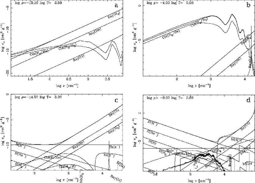
Figure 2: Absorption coefficient $\kappa_{s}(\nu)+\kappa_{a}(\nu)$ for different densities and temperatures: (a) $\rho=10^{-15}\textup{ g}\textup{ cm}^{-3}$, $T=10^{2.6}\textup{ K}$; (b) $\rho=10^{-4}\textup{ g}\textup{ cm}^{-3}$, $T=10^{3}\textup{ K}$; (c) $\rho=10^{-14}\textup{ g}\textup{ cm}^{-3}$, $T=10^{3.2}\textup{ K}$; (d) $\rho=10^{-9}\textup{ g}\textup{ cm}^{-3}$, $T=10^{3.6}\textup{ K}$. Also shown are the contributions of the different absorption processes.

Extrapolation to non-tabulated low frequencies was done according $\kappa_{\nu,\textup{\tiny CIA}}\propto\nu^{2}$. This extrapolation is justified as for given temperature at low frequencies, the absorption coefficient for CIA(A/B) (e.g. Meyer et al., 1989)

$$\alpha(\omega)=\frac{4\pi^{3}}{3hc}n_{A}n_{B}\omega g(\omega,T)\left(1-e^{-\frac{h\omega}{2\pi k_{\mathrm{B}}T}}\right)$$

is only proportional to $\lim_{\omega\to 0}\omega(1-e^{-\frac{h\omega}{2\pi k_{\mathrm{B}}T}})\propto\omega^{2}$ while the mainly used BC spectral shape (Birnbaum & Cohen, 1976; Borysow et al., 1985) is constant. In the formula above, $\omega=2\pi\nu$ is the angular frequency, $n_{A}$ and $n_{B}$ are the densities of the species in $\textup{ amagat}^{-1}$ , while $T$ denotes the temperature, $c$ the speed of light and $h$ Planck’s constant.

3.5 Neglected processes

There are more CIA data available in the literature (e.g. Borysow & Meyer, 1988; Gustafsson & Frommhold, 2001b, for CIA of HD/{He,Ar,H₂ and H}), but their maximum in absorption roughly coincides with the $\textup{H}_{2}/\textup{H}_{2}$ and $\textup{H}_{2}/\textup{He}$ CIA in position and height. Given the small number fraction of D and the kind of absorption (dipole radiation), for the abundances considered here these absorption never dominates.

3.6 Absorption coefficients

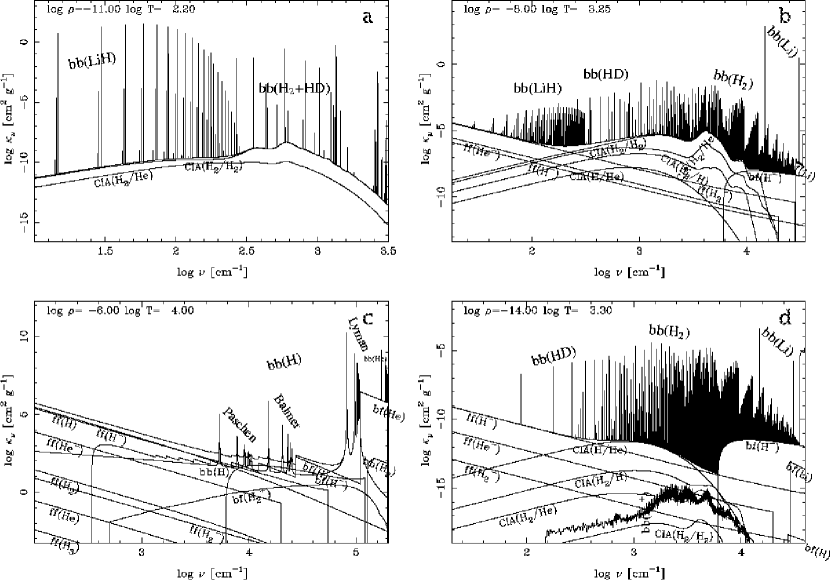
Figure 3: Absorption coefficient $\kappa_{a}(\nu)$ for different densities and temperatures including line absorption: (a) $\rho=10^{-15}\textup{ g}\textup{ cm}^{-3}$, $T=10^{2.2}\textup{ K}$; (b) $\rho=10^{-8}\textup{ g}\textup{ cm}^{-3}$, $T=10^{3.25}\textup{ K}$; (c) $\rho=10^{-6}\textup{ g}\textup{ cm}^{-3}$, $T=10^{4}\textup{ K}$; (d) $\rho=10^{-14}\textup{ g}\textup{ cm}^{-3}$, $T=10^{3.3}\textup{ K}$. Also shown are the contributions of the different absorption processes.

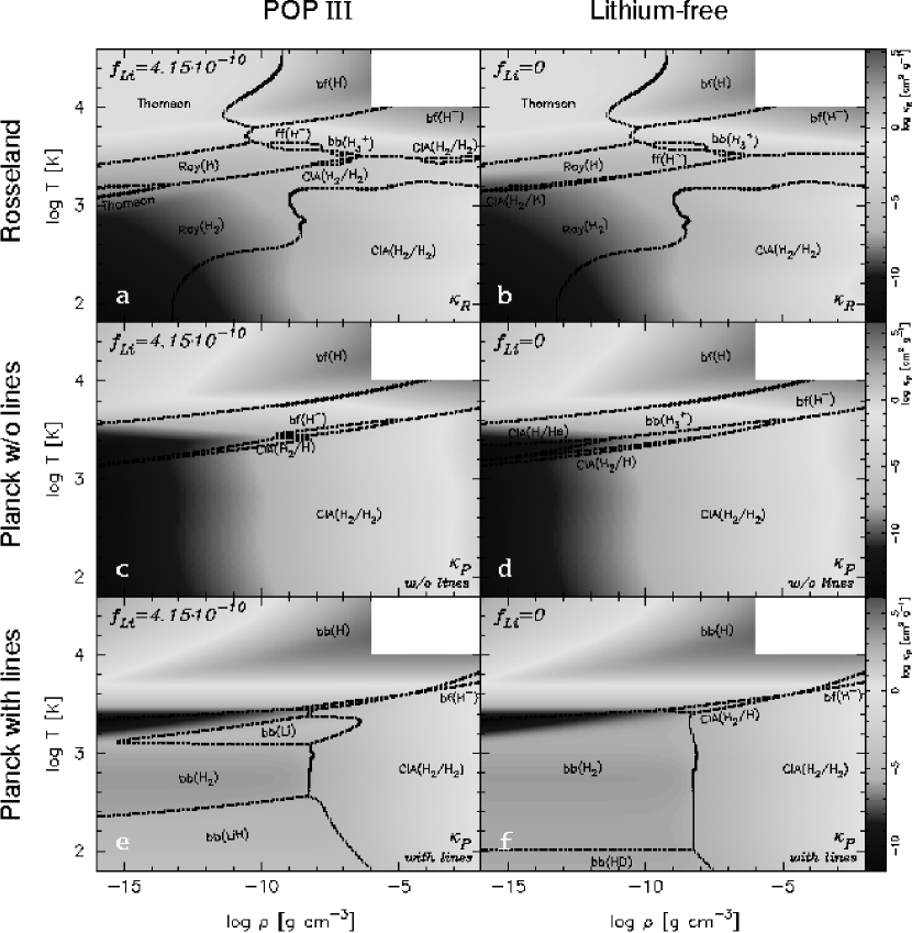
Figure 4: Rosseland (a+b) and Planck mean (without lines: c+d, with lines: e+f) values for the POP III case ($f_{\textup{Li}}=4.15\cdot 10^{-10}$, left: a,c,e) and the zero-metal case ($f_{\textup{Li}}=0$, right: b,d,f)

We calculate monochromatic continuum absorption and scattering coefficients $\kappa_{a,i}(\nu,n_{j},\rho,T)$ and $\kappa_{s,i}(\nu,n_{j},\rho,T)$ for all the 28 continuous absorption and scattering processes (see Table 3) using the cross sections $\sigma_{a/s,i}(\nu,T)$ weighted with the abundance $n_{j}(\rho,T)$ of the contributing species.

For the absorption processes we correct for stimulated emission (factor $1-exp\left(-h\nu/k_{\mathrm{B}}T\right)$, Mihalas, 1978) unless not already included in the tabulated absorption coefficents. We sum them both up and divide by the density $\rho$ to get the mass absorption and scattering coefficents $\kappa_{s}(\nu,\rho,T)$ and $\kappa_{a}(\nu,\rho,T)$ (cf. LCS91, )

$$\kappa_{a}(\nu,\rho,T) = \frac{1}{\rho}\sum_{i}\sigma_{a,1,i}(\nu,T)n_{j}(\rho,T)\left(1-e^{-\frac{h\nu}{k_{\mathrm{B}}T}}\right)$$ (1)

$$+\frac{1}{\rho}\sum_{i}\sigma_{a,2,i}(\nu,T)n_{j}(\rho,T)n_{k}(\rho,T)\left(1-e^{-\frac{h\nu}{k_{\mathrm{B}}T}}\right)$$

$$\kappa_{s}(\nu,\rho,T) = \frac{1}{\rho}\sum_{i}\sigma_{s,1,i}(\nu,T)n_{j}(\rho,T)$$ (2)

$$+\frac{1}{\rho}\sum_{i}\sigma_{s,2,i}(\nu,T)n_{j}(\rho,T)n_{k}(\rho,T)$$

The indices ”1” and ”2” indicate 1- and 2-body absorptions.

Figs. 2 and 3 show sample absorption coefficients.

4 Rosseland and Planck mean values

Using them together with the integrated line absorption coefficients (LABEL:eq:integabscoef) calculations of the Rosseland and Planck mean opacity are done according to

$$\frac{1}{\kappa_{R}(\rho,T)}=\frac{3\pi}{4\sigma T^{3}}\int_{0}^{\infty}\frac{1}{\kappa_{s}+\kappa_{a}}\frac{\partial B_{\nu}}{\partial T}d\nu$$ (3)

$$\kappa_{P}(\rho,T)=\frac{1}{\sigma T^{4}}\int_{0}^{\infty}\kappa_{a}B_{\nu}d\nu+\sum_{i}\kappa_{P,L_{i}}$$ (4)

where the factors in front of the integrals are the normalization conditions.

The typical range of our frequency grid is $10\dots 10^{7}\textup{ cm}^{-1}$ which corresponds to photon energies of $1.24\cdot(10^{-3}\dots 10^{3})\textup{ eV}$. We use typically $20000$ logartithmically equidistant grid points with additional points added for a better resolution of bound-free absorption edges.

In this contribution, calculations of Planck means are carried out for two sets: one set only including the continuum contribution and one including all contributions added via the integrated absorption coefficient. The only exceptions from this scheme are $H_{3}^{+}$, CIA and Stark broadening of atomic H. The latter obviates opacity calculation for $\rho>10^{-5}\textup{ g}\textup{ cm}^{-3}$ and $T>10^{4}\textup{ K}$.

The two Planck sets are two extreme cases, where the complete Planck opacity set (continuum+lines) can be used for “zeroth-order” calculations, while the Planck continuum is suitable for more detailed modeling (including lines depending on the motion of the gas, etc.).

4.1 Rosseland mean

The upper part of Fig. 4 shows the Rosseland means for our POP iii Li content $f_{\textup{Li}}=4.15\cdot 10^{-10}$ and the Li-free composition.

The $\rho$-T-plane can be divided into 4 regions split by the lines $\rho\approx 10^{-9}\textup{ g}\textup{ cm}^{-3}$ and $T\approx 3000\textup{ K}$. At low density scattering dominates while true absorption is dominating the high-density region. For scattering we distinguish between Rayleigh scattering and Thomson scattering (see Figs. 2a+c) in the low- and high-temperature regimes. True absorption is divided into mainly bound-free and CIA absorption (see Figs. 2d+b).

In the mid-temperature region there is a steep transition between small and large opacity values at low and high temperatures, respectively. For the low-density region the steep gradient is simply produced by the sharp decline/appearance of $\textup{H}_{2}$, H and $\textup{e}^{-}$ (evident in the dominance of scattering involving these species) while at high densities bound-free absorption of $\textup{H}^{-}$ is the dominant mechanism which itself exhibits a strong temperature dependence.

A comparison of the Li-free with the POP iii case shows the importance of taking an even minute Li contents into account (as was already indicated by the number densities in Fig. 1). The early ionisation of Li increases the $\textup{H}^{-}$ abundance which at high densities shows up as an extension of the $\textup{H}^{-}$ dominated opacity area and as an increase in the opacity value. At lower densities the free electrons increase the opacity due to Thomson scattering. The presence of Li, however, decreases the Rosseland means at intermediate densities due to the destruction of $\textup{H}_{3}^{+}$ ions. (cf., Figs. 4a and b). In Fig. 5a we show these differences quantitatively.

4.2 Planck mean

In panels c–f of Fig. 4 we show the Planck mean opacities for the Pop iii chemical composition (panels c and e) and for the Li-free mixture (d and f). In panels c and d we show the values for continuum absorption only, while in panels e and f lines are taken into account.

4.2.1 Continuum absorption

For continuum absorption the Planck means show a rather simple three-part structure approximately following the change from molecular to atomic to ionic H, respectively. In the molecular H region the only dominant true absorption is CIA of $\textup{H}_{2}/\textup{H}_{2}$ pairs, whereas for atomic H bound-free absorption of $\textup{H}^{-}$ and for ionised H bound-free absorption of H are the dominant absorption mechanisms.

Li influences the opacity in a small stripe at the boundary between the CIA ($\textup{H}_{2}/\textup{H}_{2}$) and the bound-free $\textup{H}^{-}$ absorption where the influence of CIA ($\textup{H}/\textup{He}$) and bound-bound of $\textup{H}_{3}^{+}$ decreases. The overall difference is similar to the Rosseland means, although the positive deviations are smaller, while the negative ones are much larger. At this transition there is a local minimum of the Planck mean, as $\textup{H}_{2}$ dissociates/forms, while H and $\textup{H}^{-}$ has not fully been formed/destroyed yet.

4.2.2 Line Absorption

Taking into account line absorption changes the result considerably: At regions where H is mostly in its atomic or ionic form, bound-bound transitions of atomic H yield the largest contribution to the opacity (see Fig. 3c). At lower temperatures, the opacity contribution of CIA ($\textup{H}_{2}/\textup{H}_{2}$) only remains dominant for high densities ($\rho>10^{-8}\textup{ g}\textup{ cm}^{-3}$), whereas at lower densities line absorption is the dominant mechanism (see Figs. 3a,b,d). With line absorption the local minimum of the opacity prominently shows up: The drop in opacity reaches 7 orders of magnitudes within a very small temperature interval (at $T\approx 2000\textup{ K}$) and low densities.

D is an important absorber only for temperatures below $\approx 100\textup{ K}$, as then the lowest-lying rotational transition of HD at $\approx 128\textup{ K}$ outperforms the $\textup{H}_{2}$ transition at $510\textup{ K}$ in its contribution to the Planck mean.

The direct influence of Li on the Planck means comes into play through the absorption of atomic Li (cf. Fig. 3b) and LiH (Li hydride, see Fig. 3a). Although the number density of these species is much smaller than those of D (itself being of considerably smaller abundance than H and He), they increase the opacity by one and a half orders of magnitude. The indirect influence of the $\textup{H}^{-}$ absorption and $\textup{H}_{3}^{+}$ destruction is still present.

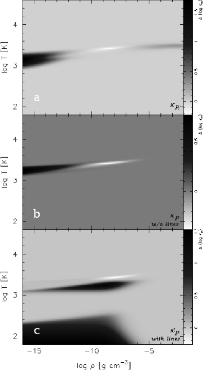
Figure 5: Difference between POP III ($f_{\textup{Li}}=4.15\cdot 10^{-10}$) and the Lithium-free case ($f_{\textup{Li}}=0$) for Rosseland and Planck mean opacities: (a) Rosseland mean; (b) Planck mean for continuum case; (c) Planck mean with lines

Atomic Li absorbs mainly through the 6708 $\AA$ transition. It is stronger than the quadrupole absorption of $\textup{H}_{2}$ through its large Einstein coefficient despite taking place at a comparatively long wavelength. However the influence of this absorption ceases with increasing temperature where Li gets ionized.

For LiH, the Einstein coefficient is larger than that of $\textup{H}_{2}$ transitions due to the presence of a strong dipole moment, but it does not reach the values of the 6708 $\AA$ transition of atomic Li. LiH becomes dominant due to the smaller energy differences spacings between its rotational levels. This considerably reduces the wavelength of the base transition. Thus the Planck function for temperatures lower than $510\textup{ K}$ (lowest rotational state of $\textup{H}_{2}$) still catches rotational and vibrational transitions of LiH (lowest rotational state at $21\textup{ K}$) while the $\textup{H}_{2}$ contribution decreases.

The double-peaked CIA dominated opacities at temperatures below $1000\textup{ K}$ can be attributed to the the isotropic overlap induced dipole and the quadrupolar field induced dipole via isotropic polarizability components in the fundamental band of $\textup{H}_{2}/\textup{H}_{2}$ (Birnbaum et al., 1996; Meyer et al., 1989, cf., our Fig. 2).

4.3 The quantitative influence of Lithium on the opacity

Here, we summarize the differences the presence or absence of Li in the chemical composition of the matter makes. In the Rosseland and Planck means Li manifests itself by

• its early ionisation;

• the destruction of $\textup{H}_{3}^{+}$ in its presence;

• the $6708\AA$ bound-bound transition of atomic Li; and by

• the molecular absorption of LiH.

The first two mechanisms show up in both the Rosseland and Planck means, while the latter only appears in the Planck line opacity. All mechanisms except the $\textup{H}_{3}^{+}$ destruction lead to an increase of the opacity.

In Fig. 6 we show for different Li fractions ($\log f_{\mathrm{Li}}=-10.3\dots-8.3$) the differences from Li-free composition.

The positive deviations ($\Delta\log\kappa>0$) show a steady increase with increasing Li content. The negative deviations (predominantly due to destruction of $\textup{H}_{3}^{+}$) increase for Li fractions $f_{Li}<5\cdot 10^{-10}$, but are being drowned by the increase of opacity for larger Li fractions.

5 A more detailed assessment of the chemical equilibrium

As we have seen, at low temperatures $\textup{H}_{2}$ is the main absorber. Due to the lack of dust which would act as a catalyst for $\textup{H}_{2}$ formation (for a comparison, see Glover, 2003), $\textup{H}_{2}$ formation and therefore cooling and absorption is small. The main $\textup{H}_{2}$ formation channels are via $\textup{H}^{-}$ and $\textup{H}_{2}^{+}$ at low and high temperatures, respectively (e.g. Galli & Palla, 1998; Lepp et al., 2002). These 2-body reactions operate on rather long timescales. However at higher densities ($n\geq 10^{8}\textup{ cm}^{-3}$) 3-body reactions become efficient (Palla et al., 1983).

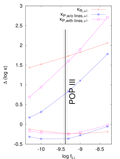
Figure 6: Deviations from Li-free ($f_{\textup{Li}}=0$) opacity for different Li contents. $\Delta\left(\log\kappa\right)>0$ indicates positive deviations, while $\Delta\left(\log\kappa\right)<0$ indicates negative deviations relative to Li-free opacity. The fiducial POP iii content is given including the uncertainties.

In the following, we look into the timescales for molecule formation in order to assess where these chemical timescales exceed the hydrodynamical one (for which we take the free-fall time scale). Thus we can estimate at which densities and temperatures the assumption of chemical equilibrium is satisfied at all.

For all timescale calculations we assume that initially the constituents of the molecules are mainly in their neutral atomic form and subsequently get converted. This approach can be justified given the fact that in the cosmological fluid H and He are in their neutral atomic form starting from a redshift of $z\approx 1100$ while for Li we take $z\approx 100$ (Galli & Palla, 1998; Lepp et al., 2002).

5.1 Molecular Hydrogen $\textup{H}_{2}$

The $\textup{H}_{2}$ formation timescale $\tau_{\textup{H}_{2}}$ due to the reaction $\textup{H}+\textup{H}+\textup{H}\rightarrow\textup{H}_{2}+\textup{H}$ can be estimated using $k_{4}$ of (Palla et al., 1983) to

$$\tau_{\textup{H}_{2}}=2420\textup{ yr}\cdot\left(\frac{T}{300\textup{ K}}\right)\left(\frac{\rho}{10^{-14}\textup{ g}\textup{ cm}^{-3}}\right)^{-2}$$ (5)

In contrast to the rapid 3-body-reaction the only relevant ionic $\textup{H}_{2}$ formation channel at low temperatures is via $\textup{H}^{-}$ while at higher temperatures $\textup{H}_{2}$ is formed via $\textup{H}_{2}^{+}$ (McDowell, 1961; Peebles & Dicke, 1968; Saslaw & Zipoy, 1967). The $\textup{H}^{-}$-consuming reaction is $\textup{H}^{-}+\textup{H}\rightarrow\textup{H}_{2}+\textup{e}^{-}$. This reaction depends on the $\textup{H}^{-}$ abundance which never is the most abundant H species and rapidly reaches chemical equilibrium as $\textup{H}^{-}$ abundance determining reactions proceed on timescales much shorter than those for the $\textup{H}_{2}$ chemistry (Abel et al., 1997). Thus taking into account the $\textup{H}_{2}$ formation rate for the ionic reaction channel is not advisable, as it would only give the timescale on which all $\textup{H}^{-}$ is depleted. The maximum $\textup{H}_{2}$ abundance due to this reaction never exceeds the available $\textup{H}^{-}$ density.

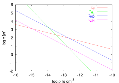
Figure 7: Comparison of free-fall timescale with the molecule formation timescales at $T=300\textup{ K}$ and a $\textup{H}_{2}$ fraction of $10^{-5}$

Following arguments similarly shown by Bromm & Loeb (2004), there exists a critical density (as a function of temperature), at which $\textup{H}_{2}$ formation proceeds within one free-fall time

$$t_{\textup{\tiny ff}}=\sqrt{\frac{3}{8\pi G\rho}}=425\textup{ yr}\cdot\left(\frac{\rho}{10^{-14}\textup{ g}\textup{ cm}^{-3}}\right)^{-\frac{1}{2}}$$

$$\rho_{\textup{crit,$\textup{H}_{2}$}}=3.2\cdot 10^{-14}\textup{ g}\textup{ cm}^{-3}\cdot\left(\frac{T}{300\textup{ K}}\right)^{\frac{2}{3}}\textup{ g}\textup{ cm}^{-3}$$

5.2 Deuterium hydride HD

HD is formed mainly via deuteron exchange with $\textup{H}_{2}$ ($\textup{H}_{2}+\textup{D}\rightarrow\textup{HD}+\textup{H}$) For the timescale we use rate coefficient (1) of Galli & Palla (2002) and get for the timescale (setting $T=300\textup{ K}$)

$$\tau_{\textup{HD}}=1.97\cdot 10^{3}\textup{ yr}\cdot\left(\frac{\rho}{10^{-14}\textup{ g}\textup{ cm}^{-3}}\right)^{-1}\left(\frac{f_{\textup{H}_{2}}}{10^{-5}}\right)^{-1}$$

Note that $\tau_{\textup{HD}}$ depends on the $\textup{H}_{2}$ fraction. Thus with increasing $\textup{H}_{2}$ abundance this timescale is reduced.

5.3 Lithium hydride LiH

For LiH we use the low-temperature rate of reaction (20) of Stancil et al. (1996) and get

$$\tau_{\textup{LiH}}=140\textup{ yr}\cdot\left(\frac{\rho}{10^{-14}\textup{ g}\textup{ cm}^{-3}}\right)^{-1}\left(\frac{T}{300\textup{ K}}\right)^{-0.28}$$

and

$$\rho_{\textup{crit, $\textup{LiH}$}}=1.08\cdot 10^{-15}\left(\frac{T}{300\textup{ K}}\right)^{-0.56}\textup{ g}\textup{ cm}^{-3}$$

The situation, however, will change, once there are data available of LiH producing 3-body reactions (see discussion in Stancil et al., 1996). This will modify the density dependence of the formation timescale ($\tau\propto\rho^{-2}$). The same applies for HD.

At densities $\rho>10^{-14}\textup{ g}\textup{ cm}^{-3}$ chemical equilibrium of $\textup{H}_{2}$ is reached within one free-fall time scale or less. Thus, for our the computational domain ($10^{-16}\textup{ g}\textup{ cm}^{-3}<\rho<10^{-2}\textup{ g}\textup{ cm}^{-3}$) the assumption of chemical equilibrium is justified, with the exception of the two lowest-density decades (which we tabulated nevertheless for computational convenience). LiH can be formed even more rapidly and thus can be regarded as being in equilibrium for densities $\rho>10^{-15}\textup{ g}\textup{ cm}^{-3}$. HD is rather hard to form, as long as there is no significant $\textup{H}_{2}$ abundance because the formation timescale crucially depends on the $\textup{H}_{2}$ fraction. However, we have seen in Sect. 4 LiH to be a significant absorber while HD is not. Thus the HD abundance is of only minor relevance for the opacities presented.

$\tau_{\textup{HD}}$, together with the other timescales discussed in this Section, is shown in Fig. 7.

6 Comparison with existing calculations

In order verify our results, we compare the Rosseland means of our calculation with existing calculations of $Z=0$ opacities by setting $f_{\textup{Li}}=f_{\textup{D}}=0$. We restrict the comparison to more recent opacities (Section 6.1-6.4). A common difference of all these opacities compared to our data can be found for temperatures around $10^{3.2\dots 3.4}\textup{ K}$. This comes about due to our use of the newly calculated $\textup{H}_{3}^{+}$ equilibrium constant in conjunction with the symmetry factor in the $\textup{H}_{2}$ dissociation equilibrium.

An overview of previous low metallicity opacities is shown in Table 4.

Reference	Opacity type	Density range	Temperature range	Chemical composition
Cox & Tabor (1976) Paczynski I-IV mixture	$\kappa_{R}$	$-12<\log\rho<-4$	$1500<T<12000\textup{ K}$	$X=0.0\dots 1.0$
Stahler et al. (1986)	$\kappa_{R}$	$-15<\log\rho<-3$	$1500<T<7000\textup{ K}$	$X=0.72$
Lenzuni et al. (1991)	$\kappa_{R/P}$	$-12<\log\rho<-0.3$	$1000<T<7000\textup{ K}$	$X=0.72$
Alexander & Ferguson (1994)	$\kappa_{R/P}$	$-7<\log R<1$	$3.0<\log T<4.1$	$X=0.0\dots 0.8$
Seaton et al. (1994) OP Project	$\kappa_{R/P}$	$-7<\log R<-1$	$3.5<\log T<8.0$	$X=0.0\dots 0.7875$
Iglesias & Rogers (1996) OPAL	$\kappa_{R}$	$-8<\log R<1$	$3.75<\log T<8.70$	$X=0.0\dots 1.0$
Harris et al. (2004)	$\kappa_{R}$	$-14<\log\rho<-2$	$1000<T<9000\textup{ K}$	$X=0.0\dots 1.0$
This work	$\kappa_{R/P}$	$-16<\log\rho<-2$	$1.8<\log T<4.6$	$X=0.75$

Table 4: Characteristics of $Z=0$ opacity calculations or opacity calculations with a $Z=0$ subset ($\rho$ in g cm^-3; $R=\rho T_{6}^{-3}$; $T$ in K; $T_{6}=T/10^{6}\,\mathrm{K}$)

6.1 Stahler et al. (1986)

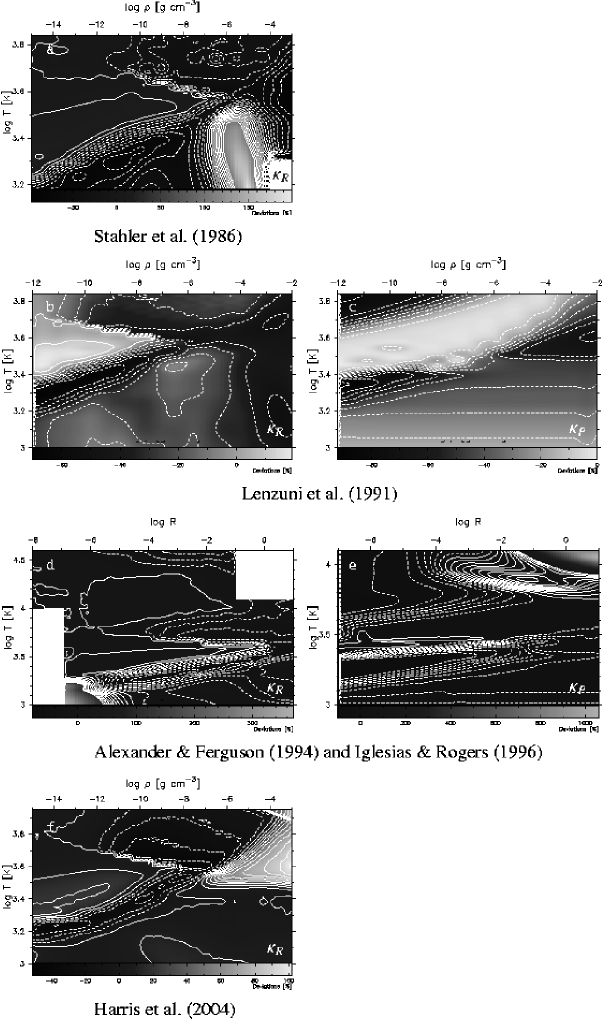
Figure 8: Comparison of our Rosseland and Planck mean opacities with previously published $Z=0$-opacities: (a) $\kappa_{\textrm{R}}$ by Stahler et al. (1986) ($X=0.72$, $Y=0.28$, and $Z=0$); (b) & (c) $\kappa_{\textrm{R}}$ and $\kappa_{\textrm{R}}$ by LCS91 ($X=0.70$, $Y=0.30$); (d) & (e) $\kappa_{\textrm{R}}$ and $\kappa_{\textrm{P}}$ by Alexander & Ferguson (1994) for $\log T<4$ ($\log T<4.1$ for Planck mean) and Iglesias & Rogers (1996) for $\log T>4$ ($X=0.70$, $Y=0.30$); (f) $\kappa_{\textrm{R}}$ by Harris et al. (2004) ($X=0.72$, $Y=0.28$). The contour lines correspond to differences of the opacity in %. Dashed lines indicate negative, solid lines positive differences relative to our opacities. The increment between neighbouring contours is 10 %.

The match with the SPS86 opacities (Fig. 8a) is good as long as $H^{-}$ is the dominant absorption mechanism. For low temperatures, the deviations are due to the use of CIA data of Linsky (1969) and Patch (1971) while we use the more recent Borysow data. The deviations at higher temperatures and densities are due to the influence of the Stark broadening of H lines which have been neglected in the SPS86 calculation.

6.2 Lenzuni et al. (1991)

The comparison with Lenzuni et al. (1991) is done for both Rosseland and Planck means (Fig. 8b&c).

At higher temperatures and densities the deviations in the Rosseland mean are again due to Stark broadened H lines. For lower temperatures the deviations are only in the 20-30 % range, much smaller than with respect to SPS86. This is due to their use of the partially newly available CIA data of $\textup{H}_{2}/\textup{H}_{2}$ and $\textup{H}_{2}/\textup{He}$ collisions for the roto-vibrational and roto-translational transitions while still having to use extrapolations for the overtones Linsky (using data by 1969).

For the Planck means the differences are considerably higher. This is due to the linearity of Planck averaging which prefers peaks in the opacity (CIA at low temperatures, H lines at higher temperatures and lower densities).

6.3 Alexander & Ferguson (1994) & Iglesias & Rogers (1996) Z=0 sets

The comparison to the OPAL opacities for the Grevesse & Noel chemical composition at Z=0 shows a much better concordance over a larger temperature range (Fig. 8d&e).

In the high-temperature limit ($\log T>3.8$) the Rosseland mean opacities are consistent at the 10% level (Stark broadening). For the very highest temperatures, deviations are due to the approximation of the statistical weight of H by the ground state which no longer is true. At lower temperatures we again have a 10-20% deviation due to CIA.

While the inclusion of Stark broadening for the Rosseland means shows a good consistence with the OPAL data, there are deviations in the Planck means. These differences are due to our coarse frequency grid which does not correctly trace all the peaks of the Hydrogen lines.

6.4 Harris et al. (2004)

The comparison to the HLMT04 data in Fig. 8f shows an overall good agreement with our data. The discussion is analogous to the OPAL comparison. except that now we are consistent at the 10% level accuracy for lower temperatures due to their use of $\textup{H}/\textup{He}$, $\textup{H}_{2}/\textup{H}$ and more recent $\textup{H}_{2}/\textup{H}_{2}$ and $\textup{H}_{2}/\textup{He}$ CIA data.

At densities $\rho>10^{-7}\textup{ g}\textup{ cm}^{-3}$ and temperatures $\log T>3.5$ there are, however, important differences. These are due to HLMT04’s use of two different approaches to calculate the $H_{3}^{+}$ abundance in order to overcome machine accuracy problems. In their $\textup{H}_{2}$ dominated regime, they take a dissociation energy of $4.52\textup{ eV}$ whereas we take $4.478\textup{ eV}$ (following Huber & Herzberg, 1979). In our calculations, we do not find any problems regarding machine accuracy. The second reason for the deviations is probably due to the difference in $\textup{H}_{2}^{+}$ absorption coefficients where we use the Stancil (1994b) data while they use Lebedev et al. (2000).

7 Conclusions

Rosseland and Planck mean opacities for primordial matter have been calculated using the most recent available data for the absorption mechanisms.

We tabulate the opacity data in Tables E1, E2 and E3, for a temperature range $1.8<\log(T/\mathrm{K})<4.6$ and $-16<\log(\rho/\mathrm{g\,\textup{ cm}}^{-3})<-2$ for our POP iii matter composition (cf. Table 1). These are the first POP iii opacity tables for temperatures $T<1000\textup{ K}$.

In order to make application as easy as possible, we provide two sets of Planck opacities: Planck means including only continuum absorption and those including molecular lines. Higher resolution tables including routines for bicubic interpolation tables are available from the authors upon request.

It has been shown (see Sect. 4 and 4.3) that the small number fraction of Li leads to a significant change in the opacity values at temperatures $T<4000\,$K compared to a pure H/He mixture. The differences can reach up to 2 orders of magnitudes. There are four processes which change the opacity:

As an alkali metal, Li gets ionized at comparatively low temperatures. It therefore increases the number of available electrons considerably. They increase the Thomson scattering contribution to the Rosseland mean at low densities while increasing the $\textup{H}^{-}$ absorption at higher densities. For both the Planck continuum and line case only the $\textup{H}^{-}$ absorption at low densities (no scattering) is enhanced.

In the presence of metals (e.g. Lithium) $\textup{H}_{3}^{+}$ is being destroyed. As $\textup{H}_{3}^{+}$ is the most abundant positive ion at temperatures around $3000\textup{ K}$ and densities $\rho>10^{-12}\textup{ g}\textup{ cm}^{-3}$ it influences the opacity indirectly in changing the chemical equilibrium when being destroyed. Furthermore, in part it shows up directly via bound-bound transitions of $\textup{H}_{3}^{+}$ at intermediate densities. For higher densities this is being drowned by the indirect increase of the $\textup{H}^{-}$-absorption.

The Planck means including line absorption are changed due to absorption by atomic Li and molecular LiH.

For atomic Li the most important transition is the $6708\AA$ feature. The Planck function, however, is most sensible to features at $6708\AA$ for temperatures of approx. $7000\textup{ K}$, a temperature at which Li is ionized, at the latest. Absorption via this transition is still important at temperatures around $1500\textup{ K}$ because the corresponding Einstein coefficient is very large compared to the quadrupole transitions of molecular and atomic H.

At temperatures $T<500\textup{ K}$ the influence of $\textup{H}_{2}$ is ceasing as the lowest lying transition of $\textup{H}_{2}$ has an equivalent temperature of $512\textup{ K}$. For lower temperatures either HD or LiH contribute to the opacities. LiH, however, has got a larger dipole moment and thus has got much larger Einstein coefficients and transitions at much lower temperatures (as low as $15\textup{ K}$).

A critical point in primordial chemistry is the formation of molecules. Formation times have been calculated for $\textup{H}_{2}$, HD and LiH. For densities $\rho\gtrsim 10^{-14}\textup{ g}\textup{ cm}^{-3}$ molecule formation proceeds within one free-fall time (except HD, which does not play any significant role in the POP iii case). Hence the calculation is valid for densities larger than that, provided the free-fall time scale being the shortest timescale relevant, other than the chemical. We give values for densities as low as $10^{-16}\textup{ g}\textup{ cm}^{-3}$ for numerical convenience.

In comparison to previous calculations we find a good agreement of our results when neglecting the newly added absorption mechanisms and the contributions of Li.

Based on our new opacities the influence of Li on the different stages of POP iii star formation and evolution can now be assessed.

acknowledgements

The authors acknowledge support from the Deutsche Forschungsgemeinschaft, DFG through grant SFB 439 (A7). Part of this work was carried out while one of the authors (MM) stayed as an EARA Marie Curie Fellow at the Institute of Astronomy, University of Cambridge, UK. The hospitality of the IoA, and of Prof. J.E. Pringle in particular, is gratefully acknowledged. The authors thank Profs. Wehrse and Gail for valuable discussions on the subject of this paper, We are grateful to Dr. Evelyne Roueff for providing the HD transition probabilities. This work has made extensive use of NASA’s Astrophysics Data System.

Appendix A EOS for Pop iii

Primordial matter is assumed to consist of a number fraction $f_{\mathrm{E}}$ of element E. Depending on the density, we define the number densities of the involved elements

$$N_{\{\textup{H},\textup{He},\textup{D},\textup{Li}\}}=\frac{\{f_{\textup{H}},1-f_{\textup{H}}-f_{\textup{D}}-f_{\textup{Li}},f_{\textup{D}},f_{\textup{Li}}\}}{4-3f_{\textup{H}}-2f_{\textup{D}}+f_{\textup{Li}}}\frac{\rho}{m_{p}}$$

We need 4 equations (6–9) to describe the conservation of the number densities of the elements (mass conservation) and an additional one (10) to take care of charge neutrality. The number density of species X is called $\left[\mathrm{X}\right]$.

$${\left[\textup{H}^{-}\right]}+{\left[\textup{H}\right]}+{\left[\textup{H}^{+}\right]}+3{\left[\textup{H}_{3}^{+}\right]}+2\left({\left[\textup{H}_{2}\right]}+{\left[\textup{H}_{2}^{+}\right]}\right) = N_{\textup{H}}$$ (6)

$${\left[\textup{He}\right]}+{\left[\textup{He}^{+}\right]}+{\left[\textup{He}^{++}\right]}+2{\left[\textup{He}_{2}^{+}\right]} = N_{\textup{He}}$$ (7)

$${\left[\textup{HD}\right]}+{\left[\textup{D}\right]}+{\left[\textup{D}^{+}\right]}+{\left[\textup{H}_{2}\textup{D}^{+}\right]} = N_{\textup{D}}$$ (8)

$${\left[\textup{LiH}\right]}+{\left[\textup{Li}\right]}+{\left[\textup{Li}^{+}\right]}+{\left[\textup{Li}^{++}\right]} = N_{\textup{Li}}$$ (9)

$${\left[\textup{e}^{-}\right]}+{\left[\textup{H}^{-}\right]}-{\left[\textup{H}^{+}\right]}-{\left[\textup{H}_{2}^{+}\right]}-{\left[\textup{H}_{3}^{+}\right]}-{\left[\textup{He}^{+}\right]}$$

$$-2{\left[\textup{He}_{2}^{+}\right]}-{\left[\textup{D}^{+}\right]}-{\left[\textup{H}_{2}\textup{D}^{+}\right]}-{\left[\textup{Li}^{+}\right]}-{\left[\textup{Li}^{++}\right]} = 0$$ (10)

Note that we neglect the H contribution of the D and L species in the H sum. Given the relative number fraction of D and Li with respect to H this assumption is satisfied. The equilibrium constants are given in Table 2.

For the A $\leftrightarrow$ B+C Saha equilibria we use equations of the form

$${}^{n}K(T)=\frac{Q_{\mathrm{B}}Q_{\mathrm{C}}}{Q_{\mathrm{A}}}\left(\xi T\right)^{\frac{3}{2}}e^{-\frac{U}{kT}}$$

with $\xi_{\textup{ion}}=2\pi m_{\textup{e}}^{-}k_{\mathrm{B}}/h^{2}=1.80\cdot 10^{10}\textup{ K}^{-1}\textup{ cm}^{-2}$ and $\xi_{\textup{diss}}=2\pi m_{\mathrm{p}}k_{\mathrm{B}}/h^{2}=3.30\cdot 10^{13}\textup{ K}^{-1}\textup{ cm}^{-2}$. $U$ is the characteristic energy for ionisation or dissociation, $Q$ the partition function of the contributing species. For $\textup{H}_{2}$-dissociation we use $\xi_{\textup{diss}}$ and correct the equilibrium constant with the symmetry factor for a homonuclear molecule (Tatum, 1966).

For the solution of the system of equations we define a critical Temperature $T_{\mathrm{crit}}=200\textup{ K}$ above which we solve the full system including the charge neutrality condition. We call this the ionic limit. Below $T_{\mathrm{crit}}$ we neglect all ions and solve (6-9) in the molecular limit.

In the ionic limit, we start with an initial guess of ${\left[\textup{e}^{-}\right]}$, solve eqns. (6-9) to derive a new ${\left[\textup{e}^{-}\right]}$ from the neutrality condition eq. (10). Iteration is done with ${\left[\textup{e}^{-}\right]}\rightarrow\sqrt{{\left[\textup{e}^{-}\right]}_{\mathrm{new}}{\left[\textup{e}^{-}\right]}_{\mathrm{old}}}$. After 20-50 iterations convergence is reached. The solution of eqns. (6-9) is done analytically and would involve a cubic equation in the case of eq. (6), otherwise only quadratic equations are involved. The cubic term in the H species equation arises due the inclusion of the $H_{3}^{+}$ abundance. As this species never is the main contributor to the number density, we neglect it in the number density conservation. Note that we also neglect the H containing D and Li species in the H conservation equation. Since we have $f_{\textup{D}}/f_{\textup{H}}\ll 1$ and $f_{\textup{Li}}/f_{\textup{H}}\ll 1$ this assumption is justified.

In the molecular limit we have to solve analytically only eqns. (6-9) neglecting ions.

Appendix B The integrated absorption coefficient

The absorption coefficient $\alpha_{\nu}$ $\left[\textup{ cm}^{-1}\right]$ for the $2\rightarrow 1$ transition can be written as

$$\alpha_{\nu}=\frac{c^{2}}{8\pi\nu^{2}}\Phi(\nu)n_{1}A_{12}\left(1-e^{-\frac{h\nu_{12}}{k_{\mathrm{B}}T}}\right),$$

where $\Phi(\nu)$ the profile function, $n_{1}$ is the number density of atoms in state 1, $A_{12}$ the Einstein coefficient and $\nu_{12}$ the transition frequency. In relation to the ground state we have

$$\alpha_{\nu}=\frac{g_{1}}{g_{0}}\frac{c^{2}}{8\pi\nu^{2}}\Phi(\nu)n_{0}A_{12}\left(e^{-\frac{E_{1}}{k_{\mathrm{B}}T}}-e^{-\frac{E_{2}}{k_{\mathrm{B}}T}}\right),$$

where $E_{1}$ and $E_{2}$ are the energies of the states relative to the ground state. In terms of the total number density $n=\sum_{i}n_{i}=\left(n_{0}/g_{0}\right)\sum_{i}g_{i}\exp(-E_{i}/k_{\mathrm{B}}T)=n_{0}Q(T)/g_{0}$

$$\alpha_{\nu}=g_{1}\frac{c^{2}}{8\pi\nu^{2}Q(T)}\Phi(\nu)nA_{12}\left(e^{-\frac{E_{1}}{k_{\mathrm{B}}T}}-e^{-\frac{E_{2}}{k_{\mathrm{B}}T}}\right).$$

Via $g_{1}A_{12}=g_{2}A_{21}$ we easily can transform to the usually used Einstein coefficient for spontaneous emission, $A_{21}$.

Evaluating $\int_{0}^{\infty}\alpha\nu d\nu$ yields ($\int_{0}^{\infty}\Phi(\nu)d\nu=1$) the integrated absorption coefficient $\chi_{\nu_{12}}$ $\left[\textup{ cm}^{-1}\textup{ s}^{-1}\right]$

$$\chi_{\nu_{12}}=g_{1}\frac{c^{2}}{8\pi\nu_{12}^{2}Q(T)}nA_{12}\left(e^{-\frac{E_{1}}{k_{\mathrm{B}}T}}-e^{-\frac{E_{2}}{k_{\mathrm{B}}T}}\right),$$

where we made use of the approximation $\nu\approx\textup{const}$ across the line.

For Planck averaging we furthermore assume $B_{\nu}\approx\textup{const}$ across the line. Then the line contribution of the $2\rightarrow 1$ transition is

$$\kappa_{P,L}(\rho,T) = \frac{1}{\rho}\frac{\int_{\nu}\alpha_{\nu}B_{\nu}d\nu}{\int_{\nu}B_{\nu}d\nu}$$

$$= \frac{1}{\sigma\rho T^{4}}\int_{\nu}\alpha_{\nu}B_{\nu}d\nu$$

$$= \frac{n}{\sigma\rho T^{4}}\sum_{\nu_{1\rightarrow 2}}\chi_{\nu_{12}}B_{\nu_{12}}$$

$$= \frac{n}{\sigma\rho T^{4}}\sum_{\nu_{1\rightarrow 2}}g_{1}\frac{1}{8\pi k_{1\rightarrow 2}^{2}Q(T)}A_{12}\left(e^{-\frac{E_{1}}{k_{\mathrm{B}}T}}-e^{-\frac{E_{2}}{k_{\mathrm{B}}T}}\right)B_{\nu}$$

$$= \frac{hcn}{4\pi\sigma\rho T^{4}Q(T)}\sum_{k_{1\rightarrow 2}}g_{1}A_{12}\left(e^{-\frac{E_{1}}{k_{\mathrm{B}}T}}-e^{-\frac{E_{2}}{k_{\mathrm{B}}T}}\right)\frac{k_{1\rightarrow 2}}{e^{\frac{hc\nu_{1\rightarrow 2}}{k_{\mathrm{B}}T}}-1}$$

where we introduced the wavenumber $k_{1\rightarrow 2}$ corresponding to the $1\rightarrow 2$ transition. Multiplied with $\rho/n$, the last expression only depends on the temperature. Calculated once for each species summing up all the lines for the temperature grid chosen, it can be added directly to the Planck mean with the density weight $n/\rho$.

Note that we make use of the Einstein coefficient $A_{12}$, which is related to the Einstein coefficient for spontaneous emission $A_{21}$ through the Einstein relation $g_{1}A_{12}=g_{2}A_{21}$.

Appendix C Equilibrium $\textup{H}_{2}^{+}+\textup{H}_{2}\leftrightarrow\textup{H}_{3}^{+}+\textup{H}$

We have fitted the equilibrium constant $\log_{10}K$ to the 6 parameter function ($x=\log_{10}(T/\textup{ K})$)

$$\log_{10}K(T)=\frac{7079\textup{ K}}{T}\left(1+\sum_{i=1}^{5}a_{i}x^{i}\right)$$

with the coefficients

$$a_{1} = +\left(0.365793\pm 0.02124\right)$$

$$a_{2} = -\left(0.624287\pm 0.03488\right)$$

$$a_{3} = +\left(0.388540\pm 0.02095\right)$$

$$a_{4} = -\left(0.102057\pm 0.00546\right)$$

$$a_{5} = +\left(0.940462\pm 0.05203\right)\cdot 10^{-2}$$

This fit causes maximum deviations of 4 $\%$ of $K$ for $300\textup{ K}<T<7000\textup{ K}$, whereas the maximum deviation never exceeds 8 $\%$ below $10^{4}\textup{ K}$. $7079\textup{ K}$ correspond to the enthalpy of $16300\textup{ K}$ for the reaction $\textup{H}_{2}^{+}+\textup{H}_{2}\rightarrow\textup{H}_{3}^{+}+\textup{H}$, divided by the $\log 10$ factor due to basis conversion.

Appendix D A remark on the standard format of opacity tables

Opacity mean values are usually tabulated in the $(R,T)$-plane, where $R=\frac{\rho}{T_{6}^{3}}$. $T_{6}$ is the temperature in units of $10^{6}$ K, $\rho$ the density. Using this $R$-parameter, the tables remain rectangular over large temperature ranges.

We have the gas ($P_{\mathrm{g}}$) and radiation ($P_{\mathrm{r}}$) pressure (here in the optically thick case)

$$P_{\mathrm{g}}=\rho\frac{kT}{\mu m_{\mathrm{p}}}\qquad P_{\mathrm{r}}=\frac{4\sigma}{3c}T^{4}$$ (12)

Calculating the ratio and taking the logarithm we have

$$\bar{\xi}=\log\left(\frac{P_{\mathrm{g}}}{P_{\mathrm{r}}}\right)=\log\left(\frac{3k_{\mathrm{B}}c}{4\sigma\mu m_{\mathrm{p}}}\right)+3\bar{T}-\bar{\rho}\approx 22.5+3\bar{T}-\bar{\rho}$$ (13)

Subtracting the logarithmized definition of $\bar{R}=\bar{\rho}+18-3\bar{T}$, we have

$$\bar{\xi}-\bar{R}=4.5$$

For $\bar{R}=-4.5$ gas and radiation pressure are equal. As the range of $\bar{R}$ usually tabulated is $-8<\bar{R}<1$ (OPAL, OP Project), $\bar{R}=-4.5$ is in the middle of this coordinate range.

The physical meaning of introducing $\bar{R}$ is that one remains in the physical regime where gas and radiation pressure compete with each other. Too large departures from this equality require changes in the EOS.

Therefore the each column of opacity tables in the style of OPAL & OP represent different gas/radiation pressure ratios.

Appendix E Sample tables

Sample tables for Rosseland and Planck means are given in Tables E1, E2 and E3 (will be available in the accepted version).

References

- Abel et al. (1997) Abel T., Anninos P., Zhang Y., Norman M. L., 1997, New Astronomy, 2, 181
- Abgrall et al. (1982) Abgrall H., Roueff E., Viala Y., 1982, A&AS, 50, 505