Jet propagation and the asymmetries of CSS radio sources

As Compact Steep Spectrum radio sources have been shown to be more asymmetrical than larger sources of similar powers, there is a high probability that they interact with an asymmetric medium in the central regions of the host elliptical galaxy. We consider a simple analytical model of the propagation of radio jets through a reasonable asymmetric environment and show that they can yield the range of arm-length and luminosity asymmetries that have been observed. We then generalize this to allow for the effects of orientation, and quantify the substantial enhancements of the asymmetries that can be produced in this fashion. We present two-dimensional and three-dimensional simulations of jets propagating through multi-phase media and note that the results from the simulations are also broadly consistent with the observations.

1 Introduction

Compact Steep-spectrum Sources (CSSs), defined to be $\stackrel{{\scriptstyle\textstyle<}}{{\sim}}$20 kpc in size (for $H_{0}$=100 km s^-1 Mpc^-1 and $q_{0}$ = 0.0) and having a steep high-frequency radio spectrum ($\alpha\geq 0.5$ where S${}_{\nu}\propto\nu^{-\alpha}$), have received a great deal of attention in recent years. The general consensus is that these are largely young sources seen at an early stage of their evolution (e.g., Carvalho 1985; Fanti et al. 1995; Readhead et al. 1996a,b; see O’Dea 1998 for a review). Related to the CSSs are the very small ($\leq 1$ kpc) Gigahertz-Peaked-Spectrum (GPS) sources (e.g., Gopal-Krishna, Patnaik & Steppe 1983; Stanghellini et al. 1998). The smallest double-lobed radio sources have been christened as the Compact Symmetric Objects (CSOs, Wilkinson et al. 1994; Readhead et al. 1996a; Taylor, Readhead & Pearson 1996; Owsianik, Conway & Polatidis 1998) which are believed to evolve into the Medium-sized Symmetric Objects (MSOs, Fanti et al. 1995) and later to the standard large double-lobed (FR II) radio sources (e.g. Snellen 2003, and references therein)

High-resolution images of CSSs (e.g. Sanghera et al. 1995; Dallacasa et al. 1995, 2002 and references therein) showed that there is a large range of structures associated with CSSs, ranging from double-lobed and triple sources to those with complex structures. Saikia et al. (1995, 2001, 2002) showed that, as a class, the CSSs were more asymmetric than larger radio sources. They also performed statistical tests of the orientation-based unified scheme, (Barthel 1989; Urry & Padovani 1995), and concluded that there were differences between the CSS radio galaxies (RGs) and quasars (QSRs) that were consistent with the unified scheme; however, there was also substantial evidence for more intrinsic asymmetries in CSSs than those which were seen for the larger sources. Arshakian & Longair (2000) studied the FR II sources in the 3CRR complete sample and also concluded that intrinsic/environmental effects are more important for sources with small physical sizes; they also found intrinsic asymmetries more important for sources of higher radio luminosities. Furthermore, while comparing the hotspot-size ratio in radio sources, Jeyakumar & Saikia (2000) found that CSSs are generally more asymmetric in this parameter as well; explaining such large ratios of hotspot sizes seems to require an intrinsic origin for the size difference.

Detailed polarization observations of individual sources, such as 3C147, show huge differential rotation measures between the two oppositely directed lobes, suggesting their evolution in an asymmetric environment (Junor et al. 1999). VLBA observations of 3C43 show evidence of high rotation measure where the jet bends sharply, suggesting collision of the jet with a dense cloud of gas (Cotton et al. 2003). The radio galaxy 3C459 has a highly asymmetric structure: the eastern component is brighter, much closer to the nucleus and is much less polarized than the western one, again suggesting interaction of the jet with a dense cloud of gas. HST images of the optical galaxy shows filamentary structures, suggestive of tidal interactions (Thomasson, Saikia & Muxlow 2003). Statistically, CSS objects exhibit a higher degree of asymmetry in the polarization of the outer lobes at cm wavelengths compared with the larger sources (Saikia & Gupta 2003; see Saikia et al. 2003 for a summary). These asymmetries in the central regions of active galaxies may be intimately related to the supply of fuel to the central engine in these objects, possibly due to interactions with companion galaxies.

Figure 1: Analytic models for jets propagating through asymmetric media: (a) the density distributions, $n(D)$, as a function of distance, with side 1 on the right and 2 on the left; since $\eta_{1}=\eta_{2}$ there is a discontinuity at $R_{2}$; (b) the arm-length ratio, $r_{D}(t)$; (c) the luminosity ratio, $r_{L}(t)$ and (d) the $r_{D}-r_{L}$ diagram, with both quantities now in log units. The open and filled circles represent the times $T_{1}$ and $T_{3}$ respectively and the open and filled triangles represent the times $T_{2}$ and $T_{4}$ respectively. The unit of time is 1 Myr.

All of these studies have indicated substantially greater asymmetries for small radio sources. It is clearly worthwhile to attempt models of their propagation so as to see if these differences can be understood. In this paper we develop a simple analytical model that enables us to treat both arm-length asymmetries and luminosity asymmetries (Section 2). We then extend the analytical model to include relativistic effects so as to allow properly for Doppler boosting and time delays if the sources are ejected closer to the line-of-sight (Section 3). In Section 4 we summarize results of our two-dimensional and three-dimensional hydrodynamical models of jets propagating through an asymmetric dense core, a symmetric galactic interstellar medium, and finally, a symmetric uniform intracluster medium (ICM). We discuss the similar results from the analytical and numerical models in Section 5.

2 Analytical Models for Jets Propagating in an Asymmetric Environment

To estimate the distances out to which jets with equal beam powers, but propagating out through different interstellar media (ISMs), would reach at various times, we further generalize the ram pressure balance calculations discussed for constant density media by Scheuer (1974) and extended to jets leaving a power-law ISM and entering intracluster media by Gopal-Krishna & Wiita (1987) and Rosen & Wiita (1988). Such models assume that the jets start with conical cross-sections and that their heads, and associated hot-spots, propagate sub-relativistically. We also estimate the ratios of radio luminosities of the two lobes as functions of time by expanding upon the calculations of Eilek & Shore (1989) and Gopal-Krishna & Wiita (1991). The latter authors suggested that an “excess” ISM in the nuclear regions (central few kpc), perhaps due to the interactions of galaxies, could lead to a larger fraction of CSS sources at higher redshifts. Such interactions could both trigger a phase of jet production from the central engine and easily lead to asymmetric distributions of gas in the inner regions for at least the $<$10⁷ yr during which the jets propagate through the galactic ISM. The propagation through denser media also implies higher efficiencies for conversion of jet power to radio luminosity (Gopal-Krishna & Wiita 1991; Blundell, Rawlings & Willott 1999); this concept is supported by the recent findings of Arshakian & Longair (2000) that more luminous sources are more asymmetric.

Our model calculations assume two intrinsically symmetric jets propagating outwards in opposite directions in pressure balance between the momentum flux density of the beam and ram pressure of the external medium, so the equation for the growth of one jet is (e.g., Scheuer 1974),

$$n(D){\left(\frac{dD}{dt}\right)}^{2} = {4KL_{b}}\over{\pi c\mu{m}_{h}{\left(D\theta\right)}^{2}}$$ (1)

where $K$ is an efficiency factor assumed to be a constant and of order unity, $\mu{m}_{h}$ is the mean particle mass where ${m}_{h}$ is the mass of the hydrogen atom, $L_{b}$ is the power of the beam, $D$ is the distance from the nucleus and $\theta$ is the full-opening angle. We assume the gas density of the interstellar medium (ISM) to be declining as

$$n(D)=\eta n_{0}\left[1+(D/a)^{2}\right]^{-\delta}.$$ (2)

For $D\gg a$, $n(D)\approx\eta n_{0}{\left(D/a\right)}^{-2\delta}.$ This approximation is assumed for the analytical model considered here. To allow for asymmetrically distributed gas in the central regions, the slopes on opposite sides of the nucleus denoted by the subscripts 1 and 2, $\delta_{1,2}$ are taken as shallower, and the core radius $a_{c}$ smaller, in the interior regions, but the slope can be steeper in the exterior regions. We have considered the possibility that the ISM density levels off to a constant ICM density at large radii. Standard central densities of $n_{0}\approx 10^{-1}$cm^-3 and $a\approx 2$ kpc are typical of large elliptical galaxies (Forman, Jones & Tucker, 1985). Excess central gas, requiring $\eta\approx 10$ and extending out to a few kpc (i.e., with $a_{c}\ll 1$ kpc) is sufficient to confine reasonably powered jets to CSS dimensions for significant lengths of time (e.g., Gopal-Krishna & Wiita 1991; Carvalho 1998).

We consider a model physically corresponding to jet propagation initially through an asymmetric nuclear region, followed by a symmetrical galactic scale ISM, and finally, through a constant ICM. The central ambient medium is characterized by $\eta=\eta_{1}$ and $\delta=\delta_{1}$ on one side, with the corresponding values on the opposite side being $\eta_{2}$ and $\delta_{2}$. For the sake of simplicity, we take the core radius for both as $a_{c}$. The jet propagating outwards on side 1 reaches a distance $R_{1}$ after a time $T_{1}$, while the one on the opposite side reaches $R_{2}$ after a time $T_{2}$. Beyond $R_{1}$ and $R_{2}$, the density distribution on both sides is described directly by equation (2), with $a\gg a_{c}$. The evolution after a distance $R_{3}(>R_{1})$ on side 1 and $R_{4}(>R_{2})$ on side 2, is governed by a constant density, with $T_{3}$ and $T_{4}$ the times taken by the corresponding jets to reach the distances $R_{3}$ and $R_{4}$, respectively (Fig. 1). Although we will usually assume $R_{2}=R_{1}$ and $R_{4}=R_{3}$, the times at which those radii are reached will be different for the opposite sides even for jets of identical powers, and it is certainly possible that $R_{2}\neq R_{1}$ or $R_{4}\neq R_{3}$, so it is useful to retain this more general notation. Quite clearly, the jet propagating through the denser side (with shallower $\delta$ or higher $\eta$) will take longer to get to any fixed distance. Note that there must be a density discontinuity, either at $D=0$ if $\eta_{1}\neq\eta_{2}$, or at $R_{2}$ if $\eta_{1}=\eta_{2}$; the latter case is shown in the left panel of Fig. 1. Such discontinuities are most likely to arise through an asymmetric distribution of gas from a recent merger that may be responsible for triggering the nuclear activity (e.g. Gopal-Krishna & Wiita 1991). However, it is relevant to note that any realistic situation would have steep gradients and not discontinuities. Note that even if $\delta>\delta_{1,2}$ (as explicitly assumed below), because $a\gg a_{c}$ the absolute rate of decline in density at $D>R_{1,2}$ is slower than at $D<R_{1,2}$ where the inner core distributions dominate.

Using Eq. (2), for $D\gg a$, equation (1) reduces to $D^{(1-\delta)}(dD/dt)=\eta^{-1/2}\tau^{-1}a^{2-\delta}$, where $\tau={\left[{\mu n_{0}c\pi{m}_{h}{\theta}^{2}}/{4KL_{b}}\right]}^{1\over 2}a^{2}.$ Integrating the above equation yields $D=[(2-\delta){\eta^{-{1\over 2}}}{\tau^{-1}}t]^{1/(2-\delta)}a$. For $D=R$ at $t=T$, this can be expressed as $D=R{({t/T})}^{1/(2-\delta)}.$ We use the above expression to estimate the distances $D_{1}$ and $D_{2}$ to the lobes 1 and 2 respectively.

When the distances of propagation of the jet on both sides satisfy $D_{1}<R_{1}$ and $D_{2}<R_{2}(=R_{1})$ then

$$D_{1,2}=R_{1,2}{({t/T_{1,2}})}^{1/(2-\delta_{1,2})}.$$ (3)

But once $D_{1}>R_{1}$,

$$D_{1}={\left[{{{2-\delta}\over{2-\delta_{1}}}\left({{t\over T_{1}}-1}\right)+1}\right]}^{1/(2-\delta)}R_{1}.$$ (4)

For $t\gg T_{1}$ this can be expressed as
$D_{1}=R_{1}\left([(2-\delta)/(2-\delta_{1})][t/T_{1}]\right)^{1/(2-\delta)}$. Similarly, for the jet propagating on the opposite side, for $D_{2}>R_{2}$,

$$D_{2}={\left[{F\left({{t\over T_{2}}-1}\right)+1}\right]}^{1/(2-\delta)}R_{2},\ \$$ (5)

with

$$F={{2-\delta}\over{2-\delta_{2}}}\left({{\eta_{2}}\over{\eta_{1}}}\right)^{1\over 2}{(a_{c}/R_{2})^{\delta_{2}-\delta}\over(a_{c}/R_{1})^{\delta_{1}-\delta}}={{2-\delta}\over{2-\delta_{2}}}\left({{a_{c}}\over{R_{1}}}\right)^{\delta_{2}-\delta_{1}},$$

where the last equality holds when $\eta_{1}=\eta_{2}$ and $R_{1}=R_{2}$. For $t\gg T_{2}$, $D_{2}=R_{2}(F/T_{2})^{1/(2-\delta)}t^{1/(2-\delta)}$.

We now estimate the ratios of separations, $r_{D}$, and luminosities, $r_{L}$, for the lobes during different stages in the evolution of the source for this model. We choose the slopes of the density distributions such that $\delta>\delta_{1}>\delta_{2}$, and $\eta_{2}=\eta_{1}$ so that $D_{1}$ is greater than or equal to $D_{2}$ when evaluated at the same time, though we leave some dependences on $\eta$ explicit in the following expressions. For $t<T_{1}$ and $t<T_{2}$, when both the jets are within the asymmetric environment, $r_{D}=[T_{2}^{1/(2-\delta_{2})}/T_{1}^{1/(2-\delta_{1})}]t^{(\delta_{1}-\delta_{2})/[(2-\delta_{1})(2-\delta_{2})]}$. Using the approximate result that the radio luminosity on each side scales as $L_{R}\propto n(D)^{3(1+\alpha)/10}\propto n(D)^{m}$ (Eilek & Shore 1989; Gopal-Krishna & Wiita 1991) we find that

$$r_{L}=\left[{\eta_{1}\over\eta_{2}}\left({R_{1}\over a_{c}}\right)^{-2(\delta_{1}-\delta_{2})}T_{1}^{2\delta_{1}\over 2-\delta_{1}}T_{2}^{-2\delta_{2}\over 2-\delta_{2}}t^{-4(\delta_{1}-\delta_{2})\over(2-\delta_{1})(2-\delta_{2})}\right]^{m},$$

where we have taken $R_{1}=R_{2}$. With $\alpha\approx 1.0,m\approx 0.6$. For the case shown in Fig. 1, where $\delta=0.75$, $\delta_{1}=0.675$ and $\delta_{2}=0.3$, $r_{D}\propto t^{0.17}$, and $r_{L}\propto t^{-0.40}$. Thus, at this early phase of the evolution, $r_{D}$ increases with time while $r_{L}$ decreases with time.

For $t\gg T_{1}$ and $t<T_{2}$,

$$r_{D}=\left({2-\delta\over 2-\delta_{1}}\right)^{1\over 2-\delta}T_{1}^{-1\over 2-\delta}T_{2}^{1\over 2-\delta_{2}}t^{\delta-\delta_{2}\over(2-\delta)(2-\delta_{2})};$$

$$r_{L}=\left[{\eta_{1}\over\eta_{2}}\left({2-\delta\over 2-\delta_{1}}\right)^{-2\delta\over 2-\delta}\left({R_{1}\over a_{c}}\right)^{2(\delta_{2}-\delta_{1})}{T_{1}^{2\delta\over 2-\delta}\over T_{2}^{2\delta_{2}\over 2-\delta_{2}}}t^{-4(\delta-\delta_{2})\over(2-\delta)(2-\delta_{2})}\right]^{m},$$

where we have used the continuity of density at $R_{1}$ to eliminate $\eta$ and $a$ through the relation $\eta a^{2\delta}=\eta_{1}a_{c}^{2\delta_{1}}R_{1}^{-2(\delta_{1}-\delta)}$. For the above values of the $\delta$’s and $m$ we see that the rise in $r_{D}$ and the decline in $r_{L}$ both become slightly stronger, with $r_{D}\propto t^{0.21}$ and $r_{L}\propto t^{-0.51}$.

For $t>T_{3}$, when the faster jet crosses $R_{3}$, the distance travelled by lobe 1 is given by

$$D_{1}={\left[{2\over{2-\delta_{1}}}\left({R_{1}\over R_{3}}\right)^{2-\delta}\left({t\over T_{1}}-{T_{3}\over T_{1}}\right)+1\right]}^{1\over 2}R_{3}.$$ (6)

For $t\gg T_{3}$ this result can be expressed as $D_{1}=R_{3}[2/(2-\delta_{1})]^{1\over 2}(R_{1}/R_{3})^{1-\delta/2}(t/T_{1})^{1/2}$.

During the last intermediate phase, when $t\gg T_{3}$ but $T_{2}\ll t<T_{4}$,

$$r_{D}=\left({2\over 2-\delta_{1}}\right)^{1/2}F^{-{1\over 2-\delta}}\left({R_{3}\over R_{1}}\right)^{\delta\over 2}T_{1}^{-{1\over 2}}T_{2}^{{1\over 2-\delta}}t^{-{\delta\over 2(2-\delta)}},$$

and

$$r_{L}=\left[\left({R_{1}\over R_{3}}\right)^{2\delta}\left({Ft\over T_{2}}\right)^{2\delta/(2-\delta)}\right]^{m}.$$

For the above choice of the parameters for the density profile, $r_{D}\propto t^{-0.30}$. Thus at moderately late times $r_{D}$ slowly decreases with time, while $r_{L}$ more rapidly approaches unity from below, since $r_{L}\propto t^{0.72}$.

Finally, once $t>T_{4}$, and the slower progressing lobe also enters the uniform intracluster medium,

$$D_{2}=\left[G\left({t\over T_{2}}-{T_{4}\over T_{2}}\right)+1\right]^{1\over 2}R_{3},$$ (7)

where

$$G={\left[{2\over 2-\delta_{2}}\left({\eta_{2}\over\eta_{1}}\right)^{1\over 2}a_{c}^{\delta_{2}-\delta_{1}}R_{1}^{\delta_{1}-\delta_{2}+2-\delta}R_{3}^{\delta-2}\right]}.$$

For $t\gg T_{4}$, this simplifies to $D_{2}=R_{3}G^{1\over 2}(t/T_{2})^{1\over 2}$. Thus, when the jets have traversed well beyond $R_{3}$ and $R_{4}$, so that $t\gg T_{3},T_{4}$, $r_{D}\longrightarrow 1$, while $r_{L}\simeq 1$ as soon as both lobes are in the constant density ICM.

In summary, the size ratio grows monotonically until $T_{2}$, after which it declines slowly toward unity. The flux-density ratio varies more dramatically, and with more complexity, dropping quite a bit until $T_{2}$ and then rising rapidly at that time, because of our assumption of a density discontinuity at $R_{2}$. Both before and after $T_{3}$, the flux-density ratio of the components becomes symmetric more rapidly than does the separation ratio, with $r_{L}\propto r_{D}^{-4m}$, but because of its earlier severe deviations from unity, it remains more asymmetric. Finally, once lobe 2 also crosses the outer interface (at $T_{4}$) and the constant density ICM is entered, the ratio $r_{L}$ very quickly approaches unity, but $r_{D}$ does so only asymptotically.

2.1 Results of basic analytical models

Fig. 1 shows the variation of density with distance from the nucleus on opposite sides, the variations of the separation ratio, $r_{D}$, and the flux density ratio, $r_{L}$, with time as the jets propagate outwards, as well as an $r_{D}$–$r_{L}$ diagram. The time axis is in units of $10^{6}$ yr. The times $T_{1}$, $T_{2}$, $T_{3}$, and $T_{4}$ when the jet crosses the interfaces at $R_{1}$, $R_{2}$, $R_{3}$, and $R_{4}$, respectively, are marked on the trajectories. Our calculations of such trajectories provide an explanation for the observed points in the $r_{D}-r_{L}$ diagram which have $r_{D}$ greater than 1 and $r_{L}$ smaller than 1 (see Saikia et al. 1995, 2001). Our calculations also show that after the jets have left the asymmetric environment, and are passing through similar media on opposite sides, the source tends to become symmetric quite rapidly. Thus most large FR II sources, which tend to be quite symmetric in both distances (cf. Arshakian & Longair 2000) and luminosities of the oppositely directed lobes, may still have passed through an asymmetric environment in early phases of their evolutions. This is consistent with the possibility that most sources may have undergone CSS phases during the early stages of their evolutions, as discussed in Section 1. In only a few of the CSS sources, such as 3C 119 (Ren-dong et al. 1991) and 3C 48 (Wilkinson et al. 1991), does it appear that the jets may have been disrupted by interaction with the clumpy external medium so that they never evolve into large sources (e.g. De Young 1993; Higgins, O’Brien, & Dunlop 1999; Wang, Wiita, & Hooda 2000).

For a specific reasonable example, consider a jet of a beam power of $7\times 10^{46}$ erg s^-1 and an opening angle of 0.04 rad, propagating through a medium with $n_{0}=1$ cm^-3, core radii $a_{c}=0.45$ kpc and $a=2.0$ kpc, with $\delta$=0.75, $\delta_{1}$=0.675, $\delta_{2}$=0.3. The times required to reach $R_{1}$=5 kpc, $R_{2}$=5 kpc, $R_{3}$=25 kpc, and $R_{4}$=25 kpc are 0.025, 0.047, 0.19, and 0.22 $\times$ 10⁶ yr, respectively. The above times for a weaker jet of power $2\times 10^{45}$ erg s^-1, with an opening angle of 0.1 radian propagating in a medium with smaller $a_{c}=50$ pc and higher central density $n_{0}=10$ cm^-3, but otherwise identical parameters, are 0.26, 1.1, 2.0 and 2.9 $\times$ 10⁶ yr, respectively. These ages are smaller than any plausible age estimates for larger sources (e.g. Leahy, Muxlow & Stephens 1989; Scheuer 1995; Blundell & Rawlings 2000). The brief times during which our models produce sources which would be classified as GPSs (well within $R_{1}$) are consistent with the different analytical approximations employed by Carvalho (1998) for jets passing through extra dense (but uniform) matter.

If there is substantially less gas on one side than the other, as is the case either if the power-law of the central fall-off is substantially less steep on one side than on the other, say $\delta_{1}-\delta_{2}\approx 0.4$, or if $\eta_{2}\approx 4\eta_{1}$, we can obtain fairly wide ranges in the predicted ratios of separations and radio luminosities, and explain the very asymmetric sources. For most sources, a modest difference in $\delta$ of about 0.15 turns out to be adequate to produce the observed asymmetries, even assuming symmetric jets of equal powers are launched from the central engine.

3 Relativistic and Viewing Angle Effects

For more detailed comparison with the observations, two other important effects must be included: the observed luminosities are boosted or depressed via possible bulk relativistic motions; and the observed positions are affected by light travel time effects.

In this section the subscript ‘a’ will denote the lobe approaching the observer and the subscript ‘r’ will denote the receding component. So $D_{a}$ and $D_{r}$ are the distances from the core to the approaching and receding lobes, respectively, while $D_{1,2}(t)$ are the distances traveled by the jets propagating through the less dense and denser media, respectively, as in the previous section; let $\varphi$ be the angle between the approaching jet and the line of sight to the observer.

In the core’s rest frame we are observing at time $t$. The corresponding times at which emission arises from the approaching/receding lobe are: $t_{a}=t/(1-\beta_{a}{\rm cos}\varphi)$; $t_{r}=t/(1+\beta_{r}{\rm cos}\varphi)$, where $\beta=v/c$. Including light travel-time effects, where the appropriate velocity is the mean speed of advance to that point, the observed distances of the approaching and receding lobes are:

$$d_{a}(t)=D_{a}(t){\rm sin}{\varphi}/(1-[D_{a}(t)/(ct)]{\rm cos}\varphi);$$

$$d_{r}(t)=D_{r}(t){\rm sin}{\varphi}/(1+[D_{r}(t)/(ct)]{\rm cos}\varphi).$$

Thus, the distance ratio, including projection and light-travel time effects is

$$r_{D}^{*}(t)\equiv{\frac{d_{a}(t)}{d_{r}(t)}}=\frac{D_{a}(t)}{D_{r}(t)}\leavevmode\nobreak\ \leavevmode\nobreak\ {\frac{1+[D_{r}(t)/(ct)]{\rm cos}\varphi}{1-[D_{a}(t)/(ct)]{\rm cos}\varphi}},$$ (8)

where the superscript $*$ indicates that relativistic effects have been included.

The luminosity corrections also will depend upon the Doppler boosting factor, which could be significant if much of the emission comes from the hotspots moving at mildly relativistic speeds, which is plausible for young sources, such as GPS and CSS objects. For a hot-spot or knot within a jet, bulk motions produce a change in flux density, so that (Scheuer & Readhead 1979)

$$S_{obs(a,r)}(\nu)=S_{em}(\nu)[\Gamma(1\mp\beta{\rm cos}\varphi)]^{-(3+\alpha)},$$

where the Lorentz factor, $\Gamma\equiv(1-\beta^{2})^{-1/2}$. The suitable values of $\beta$ are the instantaneous rates of advance of the lobes.

In the notation of §2, $S_{em}=L_{R}$ and $L_{R}\propto n(D)^{m}$. Therefore, the above equations tell us that the observed luminosity ratio is:

$$r_{L}^{*}(t)={\frac{S_{obs,a}(t)}{S_{obs,r}(t)}}={\frac{L_{R,a}(t_{a})[\Gamma_{a}^{*}(1-\beta_{a}^{*}{\rm cos}\varphi)]^{-(3+\alpha)}}{L_{R,r}(t_{r})[\Gamma_{r}^{*}(1+\beta_{r}^{*}{\rm cos}\varphi)]^{-(3+\alpha)}}}.$$ (9)

Where $\beta_{a}^{*}\equiv{\frac{1}{c}}{\frac{dD_{a}(t_{a})}{dt_{a}}}$,   $\beta_{r}^{*}\equiv{\frac{1}{c}}{\frac{dD_{r}(t_{r})}{dt_{r}}}$, and $\Gamma^{*}_{a,r}$ are determined from these instantaneous $\beta^{*}$s evaluated at the approaching (or receding) times. To evaluate this precisely, albeit in a model dependent fashion, explicit formulae for $L_{R,a}(t_{a})$ and $L_{R,r}(t_{r})$ should be used (e.g., Eilek & Shore 1989; Blundell, Rawlings & Willott 1999; Manolakou & Kirk 2002), and no further simplification is possible. However, the boosting term will typically dominate over the light-travel time factors for the luminosity ratio, even for the low values of $\beta\leq 0.2$ derived from spectral aging and other considerations (Scheuer 1995; Gopal-Krishna & Wiita 1996; Arshakian & Longair 2000). Therefore, for analytical work Eq. (9) can be approximated as

$$r_{L}^{*}(t)\simeq{\frac{L_{R,a}(t)}{L_{R,r}(t)}}\leavevmode\nobreak\ {\frac{[\Gamma_{a}^{*}(1-\beta_{a}^{*}{\rm cos}\varphi)]^{-(3+\alpha)}}{[\Gamma_{r}^{*}(1+\beta_{r}^{*}{\rm cos}\varphi)]^{-(3+\alpha)}}}.\leavevmode\nobreak\ \leavevmode\nobreak\ \leavevmode\nobreak\ \leavevmode\nobreak\ \leavevmode\nobreak\ \leavevmode\nobreak\ \leavevmode\nobreak\ \leavevmode\nobreak\ \leavevmode\nobreak\ \leavevmode\nobreak\$$ (10)

Figure 2: Evolutionary tracks for $r_{D}^{*},r_{L}^{*}$ and $r_{D}^{*}-r_{L}^{*}$ diagrams for different viewing angles to the line of sight. The upper panels are for Case 1 while the lower panels are for Case 2. The solid, dashed, dot-dashed and dotted lines indicate a viewing angle, $\varphi$, of 10, 45, 75 and 90 degrees, respectively. The symbols marking the time have same meaning as in Fig. 1, and the unit of time is 1 Myr.

3.1 Evolutionary tracks in the $r_{D}-r_{L}$ diagram

Case 1: Here we consider the situation where the jet approaching us is propagating through the less dense medium. Then both density and travel-time effects act to increase the observed arm-length ratio, $r^{*}_{D}$. However the travel-time and density induced luminosity changes work against the relativistic effects in finding the luminosity ratio, $r^{*}_{L}$. Since the side approaching us comes through a lower density medium, it is both farther out and observed at a “later” time, so that the density is even lower (or at most the same) as it was for the receding lobe; both of these effects imply a lower emissivity; however, the approaching lobe is Doppler boosted. Meanwhile, the receding lobe is still in a higher density region (at least until both have reached the ICM), and is observed at an earlier time in its history, so $n(D_{r})$ is even higher, implying relatively enhanced emissivity; but it is weakened by the Doppler effect.

Here the appropriate values are $D_{a}(t)=D_{1}(t)$ and $D_{r}(t)=D_{2}(t)$, where $D_{1,2}$ are obtained from Eqs. (3–7), with the appropriate equations used depending upon the distances the two lobes have travelled. Then, recalling that $r_{D}(t)\equiv D_{1}(t)/D_{2}(t)$ we have for the observed ratio,

$$r_{D}^{*}(t)\equiv{\frac{d_{a}(t)}{d_{r}(t)}}=r_{D}(t)\leavevmode\nobreak\ \leavevmode\nobreak\ \left[{\frac{1+[D_{2}(t)/(ct)]{\rm cos}\varphi}{1-[D_{1}(t)/(ct)]{\rm cos}\varphi}}\right].$$ (11)

and

$$r_{L}^{*}(t)\simeq r_{L}(t)\leavevmode\nobreak\ \leavevmode\nobreak\ \left[{\frac{\Gamma_{2}^{*}(1+\beta_{2}^{*}{\rm cos}\varphi)}{\Gamma_{1}^{*}(1-\beta_{1}^{*}{\rm cos}\varphi)}}\right]^{(3+\alpha)}\equiv\leavevmode\nobreak\ r_{L}(t){\cal D}_{1}(t).$$ (12)

The observed $r^{*}_{D}$ is increased more for smaller viewing angles as shown in the upper-left panel of Fig. 2. Although $r_{L}$ can be quite small at very early times, the ratio of the Doppler boosting factors, ${\cal D}_{1}$, is usually greater than unity, and this raises $r^{*}_{L}$. Even for modest $\beta(<0.2)$ it can invert the ratio and let the lobe more distant from the nucleus appear brighter if it is approaching the observer. At early times, the density effects dominate and the sources fall below the $r^{*}_{L}=1$ line, unless $\varphi$ is very small, in which case $r^{*}_{L}$ may initially exceed unity before quickly dropping below it. Later on, the value of $r_{L}$ rises above 1 for $\varphi<90^{\circ}$, and for most viewing angles the source spends a considerable amount of time within a factor of a few of the $r_{L}=1$ line, as shown in the upper-middle panel of Fig. 2. The evolutionary tracks move to the right on the $r_{L}^{*}-r_{D}^{*}$ plane as the jet points closer to the line-of-sight (Fig. 2, upper-right). Therefore, this scenario can explain sources observed to have fairly substantial ($\sim 10$) asymmetries in distance and/or luminosity; those asymmetries can be correlated or anti-correlated, depending on viewing angle and evolutionary phase.

Case 2: In this situation the side approaching us comes through the denser medium, so $D_{a}(t)=D_{2}(t)$ and $D_{r}(t)=D_{1}(t)$. Now,

$$r_{D}^{*}(t)\equiv{\frac{d_{a}(t)}{d_{r}(t)}}={\frac{1}{r_{D}(t)}}\leavevmode\nobreak\ \leavevmode\nobreak\ {\frac{1+[D_{1}(t)/(ct)]{\rm cos}\varphi}{1-[D_{2}(t)/(ct)]{\rm cos}\varphi}},$$ (13)

and

$$r_{L}^{*}(t)\simeq\frac{1}{r_{L}(t)}{\left[\frac{\Gamma_{1}^{*}(1+\beta_{1}^{*}{\rm cos}\varphi)}{\Gamma_{2}^{*}(1-\beta_{2}^{*}{\rm cos}\varphi)}\right]}^{3+\alpha}\equiv\frac{{\cal D}_{2}(t)}{r_{L}(t)}.$$ (14)

Since $1/r_{L}(t)>1$, both of the factors in the above expression enhance the luminosity ratio, $r_{L}^{*}$, and at very early times it can be very high. However, the two effects work oppositely for the arm-length ratio, $r_{D}^{*}$. Although $1/r_{D}(t)<1$, for smaller viewing angles and at very early times, $r_{D}^{*}$ can be well above unity; such sources have $r_{L}^{*}>1$ but are less asymmetric in $r_{D}^{*}$ compared to Case 1, as shown in Fig. 2. Up until $T_{2}$, $r_{D}^{*}$ falls; around then the density effects are comparable to the light travel time effects. At later times $r_{D}^{*}$ rises a bit, but by $T_{4}$ it starts to asymptotically approach unity. Although we have plotted $r_{D}^{*}$ (from Eq. 13) as less than 1 in the lower-left panel of Fig. 2, since the observed arm-length ratio is defined to be $>1$, we invert both $r_{D}^{*}$ and $r_{L}^{*}$ for the $\varphi=90^{\circ}$ curve in the bottom-right panel of Fig. 2, showing that the evolutionary track in the $r_{D}^{*}-r_{L}^{*}$ plane is similar to that of an unbeamed source (Fig. 1). A similar procedure is adopted for $\varphi=75^{\circ}$ in the time range when $r_{D}^{*}<1$. The typical outcome of this scenario is a source observed to be nearly symmetric in $r_{D}$ but possibly very asymmetric in $r_{L}$.

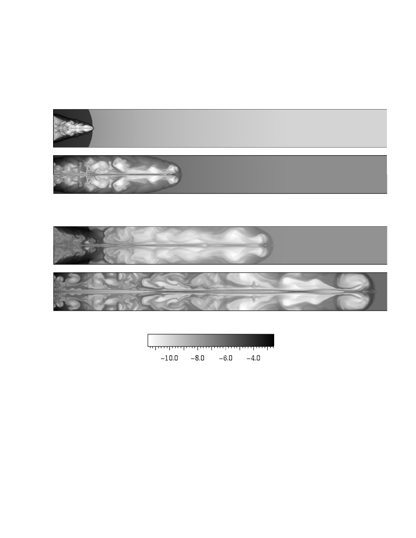
Figure 3: Two-dimensional simulations, set up to nearly reproduce our analytical model in the plane of the sky ($\varphi=90^{\circ}$). The natural logarithm of the density is shown for Runs A2 (upper image in each panel) and B2 (lower) at $t=0.80$ (top panel) and $t=2.05$ (bottom panel). The computation is conducted on the upper half of the illustrated region and symmetry about the propagation axis is assumed in plotting the density. The total length of the grid is 35 kpc, with $R_{1}=$ 5 kpc and $R_{3}=$ 25 kpc; here the unit of time is 0.6 Myr.

4 Numerical Simulations

We have examined some of our analytical estimates using numerical simulations of propagating jets. To follow the jets with very high resolution for the extended distances that are necessary if we are to examine their evolution for situations involving the multiple external media in our models, we are constrained to perform two-dimensional axisymmetric computations. To allow for some physically realistic breaking of axisymmetry, we have also performed three-dimensional simulations, albeit at lower resolution. We used the well-tested general purpose ZEUS 2D and 3D (v.3.4) codes which are described in depth in Stone & Norman (1992a,b), Stone, Mihalas, & Norman (1992), Clarke & Norman (1994), and Clarke (1996a). As we could not implement the magnetohydrodynamical version of ZEUS (e.g., Clarke 1996b), we cannot make even the quasi-realistic estimates of the source luminosities that can arise from codes that include magnetic fields. Therefore, these simulations are useful for examining $D(t)$ and $r_{D}(t)$, but not $L(t)$ or $r_{L}(t)$. We now briefly summarize results from these efforts.

4.1 2-D Simulations

For the first set of simulations we used the ZEUS 2-D code as modified by Hooda et al. (1994). Our 2-D work used cylindrical coordinates with 900 zones along the axial (jet propagation) direction and 200 zones in the radial direction. The jet radius has been scaled to 0.05 kpc, with the entire grid running from 1–35 kpc in the axial direction and 0–2 kpc in the radial direction. With these choices, 25 zones are included within the initial jet radius, and adequate resolution of internal shocks and rarefactions are achieved.

The density within the ISM exactly follows the profile as defined by Eqn. (2), and does not make the pure power-law assumption used in §2. In this work the important parameters are: the jet Mach number, ${M_{j}={u}/{a_{\rm in}}}$, with $a_{\rm in}$ the jet sound speed and $u$ the velocity of the jet; $\zeta\equiv\rho_{\rm jet}$/$\rho_{0}$, with $\rho_{0}$ the initial ambient density and $\rho_{j}$ the density of the jet. Our numerical simulations also assume initially conical jets, i.e., we set the half opening angle to 0.05 rad in these computations (cf. Wiita, Rosen & Norman 1990; Wiita & Norman 1992.)

Table 1: The parameters of the numerical runs

	2D		3D
	A2	B2	A3	B3
$\zeta$	0.001	0.001	0.001	0.001
$M_{j}$	26	26	26	26
$\theta_{j}$(radian)	0.05	0.05	0.02	0.02
$R_{1}$(kpc)	5	5	5	5
$R_{3}$(kpc)	25	25	25	25
$a_{c}$(kpc)	0.05	0.05	0.45	0.45
$a$(kpc)	1.0	1.0	2.0	2.0
$\delta$	0.75	0.75	0.75	0.75
$\delta_{1}$	$-$	0.675	$-$	0.675
$\delta_{2}$	0.3	$-$	0.3	$-$
$R_{0}$(kpc)	0.05	0.05	1.0	1.0

We performed two simulations (A2, B2, where A2 corresponds to $D_{2}$ and B2 to $D_{1}$ of Sect. 2) with parameters given in Table 1. Beyond 25 kpc both densities were constant and equal. In both cases, the jets are assumed to be in initial pressure balance with the external medium. All individual portions of the external gases are taken as isothermal and the interfaces are pressure matched; thus in Case A2 there is an abrupt density drop by a factor of 0.03 at the first interface at 5 kpc (easily seen in the uppermost panel of Fig. 3), and there is a corresponding rise in $T$ by a factor of 33 across that interface.

Figure 4: The ratios of the location of the Mach disk and bow shock of Run B2 to those of A2, $r_{D}$, as functions of time scaled to units of Myr. The triangle denotes the bow shock $r_{D}$ and the circle denotes the Mach disk $r_{D}$.

Although the code is not relativistic, the simulation can be reasonably scaled so that it is applicable to FR II radio sources. For a value of the initial jet radius $R_{0}$ = 0.05 kpc and $T_{ISM}$ = 10⁶K, one time unit corresponds to 0.6 $\times$ 10⁶yr. The velocity of the jet flow with respect to the ambient medium is $0.4c$ and the power of the jet is $L_{b}\simeq 2\times 10^{45}$ erg s^-1 for a central ambient density of $n_{0}=10$ cm^-3.

Figure 3 shows gas density for the two simulations (A2 and B2) at the same early (set of two at the top) and late (2.5 times greater; set of two at the bottom) times. The early time is chosen to correspond to the point when the slower jet (A2) just emerges from the denser inner core. At that same time, the identical jet propagating through the less dense inner core (B2) has long since blasted though its more rapidly declining inner medium ($\delta_{B2}\equiv\delta_{1}>\delta_{A2}\equiv\delta_{2}$), and has gone a good way out into the symmetric ISM. So at that time, the ratio of distances propagated is nearly maximal, since the asymmetry produced by the differences between the central media is fully felt. At the late time shown, just before the less impeded jet leaves the grid, the ratio of distances is substantially reduced, in that the early asymmetry in environment is mitigated by the longer phase of propagation through symmetric media. Figure 4 illustrates the 2-D results for $r_{D}$ defined using both the Mach disk and the bow shock positions; we see that for these simulations there is essentially no difference between them, as the jet always terminates just a short distance behind the bow shock. Since CSS sources are restricted by definition to sizes in which galactic halos and any irregularities in them will play a large role, the much greater asymmetries observed for them (as compared to substantially bigger FR II RGs) are easily accommodated.

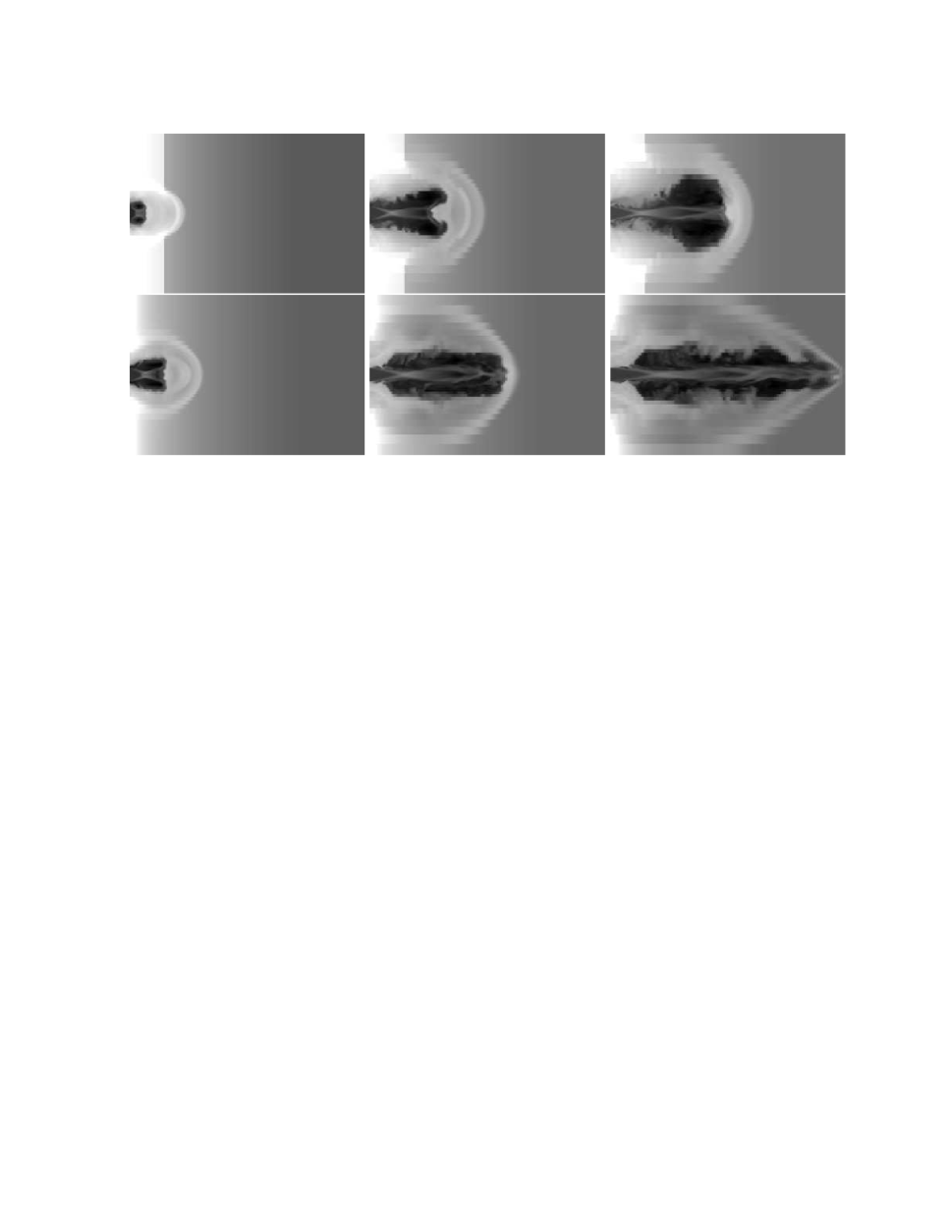
Figure 5: The natural logarithm of the density (with white the densest and black the least dense) is shown for Runs A3 (top) and B3 (bottom) at three times: $t=0.021$, left; $t=0.080$, middle; $t=0.144$, right; here the unit of time is 6.0 Myr. Note that these are slices through a 3-D computation and no symmetries are imposed, so that non-axisymmetric motions are clearly visible in the rightmost panels. The grid runs from 1–35 kpc along the propagation direction and $\pm 12$kpc in the transverse direction.

4.2 3-D Simulations

Three-dimensional simulations allow for the generation of non-axisymmetric modes and instabilities. The parameters of our 3-D simulations are also given in Table 1, and are similar to those of the 2-D simulations. The main differences are the need to use a larger values of $R_{0}$ (1.0 kpc), $a_{c}$, and $a$ and a somewhat smaller value of $\theta_{j}$, these changes being necessary to allow sufficient resolution in the necessarily coarser 3-D simulations. These three-dimensional simulations were run on 150$\times$50$\times$50 active zones, extending out to 35$R_{0}$ (35 kpc) along the initial direction of propagation, $x$, and to $\pm$12$R_{0}$ ($\pm$12 kpc) in both directions perpendicular to it. To provide marginally adequate resolution in the most important region, 14 uniform zones span the jet diameter, with the rest of the zones logarithmically scaled (e.g. Hooda & Wiita 1996; 1998). This set-up allows the jets sufficient time to propagate through each medium so that the effects of the different ambient media on the jets can be ascertained; see Saikia et al. (2003). We believe these to be the first 3-D extragalactic jet simulations to employ non-zero opening angles.

With the exception of a relatively wider jet (in comparison to the size of the core and main galaxy, which is required to provide adequate resolution within the jet), and minor differences in the scale heights, the parameters for the first two 3-D simulations are identical to those of the 2-D simulations. Therefore we can quite quickly see the differences produced by adding a third dimension.

Figure 5 displays densities from simulations A3 and B3 at early, middle and late times in the evolutions. For a canonical value of $R_{0}$ = 1 kpc and $T_{\rm ISM}=10^{6}$K, the unit of time is now 6.0 $\times$ 10⁶ yr. A major difference between the 2-D and 3-D runs is that the bow shocks run ahead of the Mach disks by much greater amounts in 3-D than they do in 2-D. At early times, when the jet is still in a transient initial state, the bow shocks for these $M_{j}=26$ jets proceed out through the inner halo very quickly, and open a large gap between the bow shocks and the working surfaces at the ends of the jets. Our analytical models assume that these two locations stay very close together, so these simulations reveal that this assumption is an oversimplification for such high Mach numbers and low jet densities. A similar behaviour is also seen in axisymmetric simulations, using a different 3-D code, of very light cylindrical jets propagating through constant density media (Krause 2003).

The finite opening angles are fairly well preserved in the first phases of the evolution (both in the central halo and for some distance into the more steeply declining ISM), despite the presence of a recollimation shock. Once the jets are at a substantial distance into the ISM, the jet becomes better collimated and then propagates nearly as a cylinder (see the middle panel of Fig. 5 for B3 and the right panel for A3). At this point, our analytical models, which assume the opening angle stays constant, lose more of their validity, as the slowing down of propagation predicted by the spreading jet picture is replaced by a situation of more nearly constant velocity. We see a slow breaking of axisymmetry through these simulations, despite the symmetric initial conditions. This can be attributed primarily to numerical errors introduced by our setting up of a conical flow within a relatively coarse Cartesian grid. Unsurprisingly, the non-axisymmetric effects are stronger for A3, which crosses a density jump; such a discontinuity helps to induce the growth of perturbations (cf. Hooda & Wiita 1996, 1998).

Figure 6: The arm-length ratios, $r_{D}(t)$ defined for both the bow shock and Mach disk locations of Runs A3 and B3 as functions of time rescaled to units of Myr. The triangles denote the bow shock ratio and the circles denote the Mach disk ratio.

Figure 6 shows the arm-length ratio, $r_{D}(t)$ for B3 to A3; this is plotted using both the bow-shock locations and the Mach disk locations. We see that the Mach-disk ratio basically follows the trend we would expect, with a substantial increase at early times while the faster jet escapes the denser core and enters the ISM, and then a more gradual decline after both jets reach the ISM. Unfortunately, our simulations could not be followed long enough to see the ratio continue to decline once both jets were in the constant density ICM, as the faster one leaves the grid before the slower one gets to that second interface (Fig. 6). The bow-shock ratio is less variable, but, after first rising, and then slightly declining, it again rises at moderate times as the Mach disk in B3 catches up with the bow shock, while the Mach disk in A3 is only starting to do so. These simulations can be scaled so as to fit FR II radio sources. For a temperature of the external gas of about $10^{6}$K, the velocity of the jet with respect to the ambient medium is $0.4c$ and the power of the jet is $L_{b}\sim 7\times 10^{46}$ erg s^-1 for a central ambient density of $n_{0}=1$ cm^-3. We have used this value of $L_{b}$ in our analytical calculations (§2 and 3) for scaling the time units.

5 Discussion and Conclusions

The asymmetric models considered above can explain the observed trend in the asymmetry parameters $r_{D}$ and $r_{L}$ (Saikia et al. 1995, 2003; Arshakian & Longair 2000). Our model for jets in an asymmetric environment oriented in the plane of the sky explains the large number of galaxies and quasars having $r_{D}>1$ and $r_{L}<1$. Our simulations of the jets propagating in asymmetric environments show a similar trend in arm-length asymmetry as that produced in our analytical calculations. We note that the observed ranges of $r_{D}$ and $r_{L}$ can be easily accommodated with the kind of asymmetric density profile discussed here. The inclusion of time-delay and Doppler boosting effects can explain the rarer sources with $r_{L}>1$, and the fact that these are relatively more common for CSS quasars (presumably seen at smaller $\varphi$) than for CSS radio galaxies.

Although our analytical model for radio source evolution is certainly oversimplified, somewhat more sophisticated models (e.g. Kaiser, Dennett-Thorpe & Alexander 1997; Blundell et al. 1999; Manolakou & Kirk 2002; Barai et al. 2004), yield similar trends for distances and radio powers with jet power, external medium density and time. Larger differences emerge at late times and at high redshifts, when different treatments of adiabatic losses and our neglect of inverse Compton losses become important; however, these are not relevant for the young CSS sources, since the synchrotron losses from these compact lobes will always exceed the inverse Compton losses (e.g., Blundell et al. 1999). The key advantage our simple model has over those more complicated approaches is that we avoid the necessity of performing numerical integrals to obtain values for $L_{R}$, so the estimates of Sects. 2 and 3 are thus possible.

Although the analytical and numerical models agree in a qualitative sense, it is not surprising that there are differences between the analytical and the numerical calculations for the arm-length ratio. Both the 2-D and 3-D numerical simulations show a peak value for $r_{D}$ of about 2.7. At later times the numerically estimated $r_{D}$’s seem to approach asymptotic values greater than 1, although the simulations could not be continued long enough to confirm this. The analytical maximum $r_{D}$ is about 1.7. The time taken to reach the first interface is similar in both analytical and numerical calculations, but in the simulations the second interface is reached later compared to the times they are reached in the analytical calculations. This implies that even though the calculated and simulated velocities are similar at early times, the velocity of the numerical jet, particularly for the 3-D case, is slower than our simple ram pressure balance calculations would indicate. These lower velocities in the numerical simulations can be understood because the effective working surface in the simulations is somewhat larger than the analytical model’s jet width, particularly at early times. These slower speeds, which are more pronounced for the jet propagating through the denser gas, also explain most of the discrepancies between the maximum values attained by $r_{D}$, and the longer times needed for $r_{D}$ to decrease towards unity.

A possible reason why the jet in the 3-D simulation slows even more with respect to the analytical estimate is that the simulated jet becomes elliptical and rotates about its own axis, as expected from theoretical calculations of the fastest growing perturbations (e.g. Hardee, Clarke & Howell 1995). The jet eventually produces an oblique Mach disk, effectively making the jet thrust smaller while narrowing the transverse width of the Mach disk (e.g. Norman 1996; Hooda & Wiita 1996). Thus, allowing for non-axisymmetry in the computations basically acts to preserve the asymmetry in $r_{D}$, and could explain the larger asymmetry seen in these simulations as well as the slower velocities at later times, as compared to the simplified analytical calculations.

Recently Carvalho & O’Dea (2002a,b) compared the propagation of jets of many different values of $\zeta$ and $M_{j}$. These simulations also used the ZEUS 2-D code and were restricted to axisymmetry, but they considered both propagation through constant density media and declining power laws. Although several parameters are different from our study, we made rough estimates of arm-length ratios using their high $M_{j}$ simulations through an ambient medium of constant density ($\delta=0.0$), and declining density ($\delta=0.75$), at a time of 0.5 Myr; $r_{D}$ is about 2.0, 1.3 and 1.1 for $\zeta$ of 0.0276, 0.0542 and 0.1106, respectively. The ranges of the observed $r_{D}$ thus argue for a small $\zeta(<0.01)$ for extragalactic radio jets. Such low $\zeta$ values have long been known to be favoured by the observed widths of cocoons seen in FR II radio sources (Norman et al. 1982).

Carvalho (1998) performed analytical calculations of jets “scattering” or penetrating through clouds in an otherwise uniform medium; the asymmetry is produced due to the statistical variance in the number of clouds the jets cross through. The arm-length asymmetry produced in his model decreases as the jet propagates forward but the symmetrization occurs at much smaller scales. To explain the corresponding flux density ratios would require the shorter arm to be colliding with a cloud at the time of observation or at least the presence of more contrast in densities between the clouds and regular ISM on the side with the shorter arm (Saikia et al. 1995, 2002). In our simulations the asymmetry builds up as time progresses before getting symmetrized at much later times with the corresponding flux density ratio changing in the correct sense.

Recent 3-D simulations of jet/cloud interactions typically either show the jets destroying the clouds or being halted by them; for a small range of jet/cloud parameters, some highly distorted structures and deflected arms can be produced (Higgins et al. 1999; Wang et al. 2000). Such simulations may be applicable to only a small number of CSSs. These cloudy medium models can confine the CSS sources to sub-galactic sizes with ages of the order of the larger radio sources (Carvalho 1998). But most observational evidence (Fanti et al. 1995; Readhead et al. 1996a,b; Pihlström et al. 2003) suggests that the CSS sources are young, not “frustrated”. Our model predictions fit the observational studies connecting CSS sources with both youth and higher degrees of asymmetry.

An analysis of the breaks in the spectra of 50 CSS sources, which included many measurements at 230 GHz, supports the picture that they are very young, with most having estimated ages of $<10^{5}$yr (Murgia et al. 1999). Our models correspond to ages in the observationally estimated ranges of $<10^{5}$–$10^{6}$yr. Our models also have the key advantage of producing the types of asymmetries in arm-lengths and luminosities that are characteristic of smaller sources.

- (1) Arshakian, T. G., Longair, M. S. 2000, MNRAS, 311, 846
- (2) Barai, P., Gopal-Krishna, Osterman, A., Wiita, P. J. 2004, BASI, in press (astro-ph/0411096)
- (3) Barthel, P.D. 1989, ApJ, 336, 606
- (4) Blundell, K. M., Rawlings, S. 2000, AJ, 119, 1111
- (5) Blundell, K. M., Rawlings, S., Willott, C. J. 1999, AJ, 117, 677
- (6) Carvalho, J. C. 1985, MNRAS, 215, 463
- (7) Carvalho, J. C. 1998, A&A, 329, 845
- (8) Carvalho, J. C., O’Dea, C. 2002a, ApJ, 141, 331
- (9) Carvalho, J. C., O’Dea, C. 2002b, ApJ, 141, 371
- (10) Clarke, D. A., 1996a, ApJ, 457, 291
- (11) Clarke, D. A., 1996b, in Energy Transport in Radio Galaxies and Quasars, ASP Conf. Ser. 100, ed. P. E. Hardee, A. H. Bridle & J. A. Zensus (San Francisco: ASP), 311
- (12) Clarke, D.A., Norman, M.L. 1994, LCA Preprint # 7 (University of Illinois, Urbana–Champaign)
- (13) Cotton, W.D., Spencer, R.E., Saikia, D.J., Garrington, S.T. 2003, A&A, in press
- (14) Dallacasa D., Fanti C., Fanti R., Schilizzi R. T., & Spencer R. E. 1995, A&A, 295, 27
- (15) Dallacasa, D., Tinti, S., Fanti, C., Fanti, R., Gregorini, L., Stanghellini, C., Vigotti, M., 2002, A&A, 389, 115
- (16) De Young, D. S. 1993, ApJ, 402, 95
- (17) Eilek, J., Shore, S. 1989, ApJ, 342, 187
- (18) Fanti C., Fanti, R., Dallacasa, D., Schilizzi, R. T., Spencer, R. E., Stanghellini, C. 1995, A&A, 302, 317
- (19) Forman, W., Jones, C., Tucker W. 1985, ApJ, 293, 102
- (20) Gopal-Krishna, Patnaik, A. R., Steppe, H. 1983, A&A, 123, 107
- (21) Gopal-Krishna, Wiita, P. J. 1987, MNRAS, 226, 531
- (22) Gopal-Krishna, Wiita, P. J. 1991, ApJ, 373, 325
- (23) Gopal-Krishna, Wiita, P. J. 1996, ApJ, 467, 191
- (24) Hardee, P.E., Clarke, D. A., Howell, D. A. 1995, ApJ, 441, 644
- (25) Higgins S. W., O’Brien T. J., Dunlop J. S. 1999, MNRAS, 309, 273
- (26) Hooda, J. S., Mangalam, A. V., Wiita, P. J. 1994, ApJ, 423, 116
- (27) Hooda, J. S., Wiita, P. J. 1996, ApJ, 470, 211
- (28) Hooda, J. S., Wiita, P. J. 1998, ApJ, 493, 81
- (29) Jeyakumar, S., Saikia, D. J. 2000, MNRAS, 311, 397
- (30) Junor, W., Salter, C.J., Saikia, D.J., Mantovani, F., & Peck, A.B. 1999, MNRAS, 308, 955
- (31) Kaiser, C. R., Dennett-Thorpe, J., Alexander, P. 1997, MNRAS, 292, 723
- (32) Krause, M. 2003, A&A, 398, 113
- (33) Leahy J.P., Muxlow T.W.B., Stephens P.W. 1989, MNRAS, 239, 401
- (34) Manolakou, K., Kirk, J. G. 2002, A&A, 391, 127
- (35) Murgia, M., Fanti, C., Fanti, R., Gregorini, L, Klein, U., Mack, K.-H., & Vigotti, M. 1999, A&A, 345, 769
- (36) Norman, M. L. 1996, in Energy Transport in Radio Galaxies and Quasars, ASP Conf. Ser. 100, ed. P. E. Hardee, A. H. Bridle & J. A. Zensus (San Francisco: ASP), 319
- (37) Norman, M. L., Smarr, L. L., Winkler, K.-H. A., Smith, M. D. 1982, A&A, 113, 285
- (38) O’Dea, C. P. 1998, PASP, 110, 493
- (39) Owsianik, I., Conway, J. E., Polatidis, A. G. 1998, A&A, 336, L37
- (40) Pihlström, Y. M., Conway, J. E., Vermeulen, R. C. 2003, A&A, 404, 871
- (41) Readhead, A.C.S., Taylor, G.B., Xu, W., Pearson, T.J., Wilkinson, P.N., Polatidis, A.G. 1996a, ApJ, 460, 612
- (42) Readhead, A.C.S., Taylor, G.B., Pearson, T.J., & Wilkinson, P.N. 1996b, ApJ, 460, 634
- (43) Ren-dong N., et al. 1991a, A&A, 245, 449
- (44) Rosen, A., Wiita, P.J. 1988, ApJ, 330, 16
- (45) Saikia, D. J., Jeyakumar, S., Wiita, P. J., Sanghera, H. S., Spencer, R. E. 1995, MNRAS, 276, 1215
- (46) Saikia, D. J., Jeyakumar, S., Salter, C. J., Thomasson, P., Spencer, R. E., Mantovani, F. 2001, MNRAS, 321, 37
- (47) Saikia, D. J., Thomasson, P., Spencer, R. E., Mantovani, F., Salter, C. J., Jeyakumar, S. 2002, A&A, 391, 149
- (48) Saikia, D.J., Jeyakumar, S., Mantovani, F., Salter, C.J., Spencer, R.E., Thomasson, P., Wiita, P.J. 2003, PASA, 20, 50
- (49) Saikia, D.J., Gupta, N. 2003, A&A, 405, 499
- (50) Sanghera, H. S., Saikia, D. J., Lüdke, E., Spencer, R. E., Foulsham, P. A., Akujor, C. E., Tzioumis, A. K. 1995, A&A, 295, 629
- (51) Scheuer, P. A. G. 1974, MNRAS, 166, 513
- (52) Scheuer, P.A.G., Readhead, A.C.S. 1979, Nature, 277, 182
- (53) Scheuer, P. A. G. 1995, MNRAS, 277, 331
- (54) Snellen, I.A.G., Mack, K.-H., Schilizzi, R.T., Tschager, W. 2003, PASA, 20, 38
- (55) Stanghellini C., O’Dea C. P., Dallacasa D., Baum S. A., Fanti R., Fanti C. 1998, A&AS, 131, 303
- (56) Stone, J. M., Norman, M. L. 1992a, ApJS, 80, 753
- (57) Stone, J. M., Norman, M. L. 1992b, ApJS, 80, 791
- (58) Stone, J. M, Mihalas, D., Norman, M. L. 1992, ApJS, 80, 819
- (59) Taylor, G. B., Readhead, A. C. S., Pearson, T. J. 1996, ApJ, 463, 95
- (60) Thomasson, P., Saikia, D.J., Muxlow, T.W.B. 2003, MNRAS, 341, 91
- (61) Urry, C. M., Padovani, P. 1995, PASP, 107, 803
- (62) Wang, Z., Wiita, P. J., Hooda, J. S. 2000, ApJ, 534, 201
- (63) Wiita, P. J., Norman, M. L. 1992, ApJ, 385, 478
- (64) Wiita, P. J., Rosen, A., Norman, M. L. 1990, ApJ, 350, 545
- (65) Wilkinson, P. N., Tzioumis, A. K., Benson, J. M., Walker, R. C., Simon, R. S., Kahn, F. D. 1991, Nature, 352, 313
- (66) Wilkinson, P. N., Polatidis, A. G., Readhead, A. C. S., Xu W., Pearson T. J. 1994, ApJ, 432, L87