The Phoenix Deep Survey: the clustering and the environment of Extremely Red Objects

Abstract

In this paper we explore the clustering properties and the environment of the Extremely Red Objects (EROs; $I-K>4$ mag) detected in a $\approx 180\rm\,arcmin^{2}$ deep ($Ks\approx 20$ mag) $Ks$-band survey of a region within the Phoenix Deep Survey, an on-going multiwavelength program aiming to investigate the nature and the evolution of faint radio sources. Using our complete sample of 289 EROs brighter than $Ks=20$ mag we estimate a statistically significant ($\approx 3.7\sigma$) angular correlation function signal with amplitude $A_{w}=8.7^{+2.1}_{-1.7}\times 10^{-3}$ (assuming $w(\theta)=A_{w}\,\theta^{-0.8}$, with $\theta$ in deg), consistent with earlier work based on smaller samples. This amplitude suggests a clustering length in the range $r_{o}=12-17\,h^{-1}\rm\,Mpc$, implying that EROs trace regions of enhanced density. Using a novel method we further explore the association of EROs with galaxy overdensities by smoothing the $K$-band galaxy distribution using the matched filter algorithm of Postman et al. (1996) and then cross-correlating the resulting density maps with the ERO positions. Our analysis provides direct evidence that EROs are associated with overdensities at redshifts $z\gtrsim 1$. We also exploit the deep radio 1.4 GHz data (limiting flux $60\mu$Jy) available to explore the association of EROs and faint radio sources and whether the two populations trace similar large scale structures. Cross-correlation of the two samples (after excluding 17 EROs with radio counterparts) gives a $2\sigma$ signal only for the sub-sample of high-$z$ radio sources ($z>0.6$). Although the statistics are poor this suggests that it is the high-$z$ radio sub-sample that traces similar structures with EROs.

1. Introduction

The study of the class of Extremely Red Objects (EROs; $I-K\gtrsim 4$ mag; e.g. Cimatti et al. 2002; Roche et al. 2002, 2003) has gained significant impetus over the last few years with the realisation that they can provide valuable information on galaxy evolution and formation scenarios (c.f. Zepf 1997; Barger 1999; Rodighiero et al. 2001; Daddi et al. 2000; Roche et al. 2002; Väisänen & Johansson 2004a, b). The very red colours of these objects suggest that they comprise evolved galaxies at redshifts $z\gtrsim 1$, the progenitors of present-day ellipticals. Study of the properties of such high-$z$ systems can indeed provide tight constraints on competing elliptical galaxy formation scenarios: monolithic collapse early in the Universe ($z_{f}>2-3$) followed by passive evolution (e.g. Eggen et al. 1962; Larson 1975) versus hierarchical merging and relatively recent formation epochs (Baugh et al. 1996; Kauffmann 1996).

Spectroscopic follow-up observations of either complete ERO samples (Cimatti et al. 2002; Cimatti et al. 2003) or individual systems (Dunlop et al. 1996; Spinrad et al. 1997; Stanford et al. 1997) have indeed confirmed that a large fraction of EROs ($\approx 50$ per cent) have absorption-line spectra. In addition to early type galaxies however, these follow-up programs also showed that a significant fraction of high-$z$ dust-shrouded active galaxies (starburst or AGNs) are also present among EROs (Cimatti et al. 1998; Dey et al. 1999; Afonso et al. 2001; Smith et al. 2001; Brusa et al. 2002).

Although the relative mix between early type and dusty systems remains poorly constrained, EROs have strong spatial clustering which is comparable if not larger than that of present day luminous ellipticals (Daddi et al. 2000, 2001, 2003; Firth et al. 2002; Roche et al. 2002, 2003). This may be interpreted as evidence that the populations of distant EROs and nearby ellipticals may be evolutionary linked. Study of the clustering of EROs, usually quantified via the 2-D correlation function, can indeed provide valuable information on the nature of these systems, their formation and evolution history as well as their environment (e.g. Daddi et al. 2001; Roche et al. 2002, 2003). Comparison of the clustering properties of EROs with those of local E/S0 may provide important insights into the evolution of early-type galaxies out to $z\gtrsim 1$.

In this paper we explore the clustering properties and the environment of EROs detected in a $\approx 180\,\rm arcmin^{2}$ deep ($Ks\approx 20$ mag) $Ks$-band survey carried out as part of the Phoenix Deep Survey (Hopkins et al. 2003), a large multiwavelength program aiming to investigate the nature and the evolution of faint (sub-mJy and $\mu$Jy) radio sources. Compared to previous studies of the clustering of EROs, the present sample has the advantage of depth combined with wider area providing a large sample of EROs to $Ks\approx 20$ mag. This is essential to increase the sample size and to improve the statistical reliability of the results compared to previous studies at similar depths (e.g. Roche et al. 2002, 2003). We caution the reader however, that although our survey is larger than previous samples at comparable magnitude limits, cosmic variance is an issue and may affect our correlation amplitude measurements. Much larger, degree scale, $K$-band surveys are required to address this issue (e.g. NOAO Deep Wide Survey; Brown et al. 2003). Our contiguous $Ks$-band survey also allows study of the association of EROs with regions of enhanced galaxy density. Indeed, although EROs are believed to reside in dense regions there is still no direct link between EROs and galaxy overdensities. The overlap of our sample with the ultra-deep and homogeneous radio observations of the Phoenix Deep Survey provides a unique opportunity to investigate the association of the radio and the ERO populations and how they trace the underlying mass distribution.

Section § 2 presents the data used in this paper and describes the selection of the ERO sample. The angular correlation function analysis is given in § 3. § 4 outlines our analysis on the environment of EROs and § 5 presents the cross-correlation of our ERO sample with the faint radio population. Finally our results are discussed and our main conclusions are summarised in § 6. Throughout the paper we adopt $\rm H_{o}=70\,km\,s^{-1}\,Mpc^{-1}$, $\rm\Omega_{M}=0.3$ and $\rm\Omega_{\Lambda}=0.7$. To allow comparison with previous studies all the distant dependent quantities are given in units of $h=\rm H_{o}/100$.

2. The Phoenix Deep Survey

2.1. Radio and NIR/Optical data

The Phoenix Deep Survey (PDS) is an on-going survey studying the nature and the evolution of sub-mJy and $\rm\mu$Jy radio galaxies. Full details of the existing radio, optical and near-infrared data can be found in Hopkins et al. (2003) and Sullivan et al. (2004); here we summarise the salient details. The radio observations were carried out at the Australia Telescope Compact Array (ATCA) at 1.4 GHz during several campaigns between 1994 and 2001, covering a 4.56 square degree area centered at RA(J2000)=$01^{\rm h}11^{\rm m}13^{\rm s}$ Dec.(J2000)=$-45\arcdeg 45\arcmin 00\arcsec$. A detailed description of the radio observations, data reduction and source detection are discussed by Hopkins et al. (1998, 1999, 2003). The observational strategy adopted resulted in a radio map that is homogeneous within the central $\rm\approx 1\,deg$ radius, with the $1\sigma$ rms noise increasing from $\rm 12\mu Jy$ in the most sensitive region to about $\rm 90\mu Jy$ close to the edge of the $\rm 4.56\,deg^{2}$ field. The radio source catalogue consists of a total of 2148 radio sources to a limit of 60 $\rm\mu$Jy (Hopkins et al. 2003).

$Ks$-band near-infrared data of the central region of the PDS were obtained using the SofI infrared instrument at the 3.6 m ESO New Technology Telescope (NTT). The observational strategy and details of the data reduction, calibration and source detection are described by Sullivan et al. (2004). The $Ks$-band mosaic covers a $\rm 13.5\times 13.3\,arcmin^{2}$ area with a 45 min integration time, and a central $\rm 4.5\times 4.5\,arcmin^{2}$ subregion which has an effective exposure time of 3 h. The completeness limit is estimated to be $Ks\approx 20$ mag for the full mosaic and $Ks\approx 20.5$ mag for the deeper central subregion.

Deep multicolour imaging ($UBVRI$) of the PDF has been obtained using the Wide Field Imager at the AAT on 2001 August 13 and 14 ($BVRI$-bands) and the Mosaic-II camera on the CTIO-4m telescope on 2002 September 3 ($U$-band), fully overlapping the SofI $Ks$-band survey. Full details on the data reduction, calibration and source detection are again presented in Sullivan et al. (2004). In this study we will use the $I$-band observations these being the deepest ($I\approx 24.2$ mag; see next section) and most appropriate for identifying EROs.

Figure 1.— $Ks$-band galaxy counts from the SofI survey survey of the PDS (filled circles). Also shown are the $Ks$-band number counts from Glazebrook et al. (1994; stars) and from the Hawaii Deep (HDS; crosses) and Medium Deep (HMDS; open circles) surveys presented by Gardner, Cowie & Wainscoat (1993).

2.2. The ERO sample

The $Ks$-band selected catalogue was constructed using SExtractor (Bertin & Arnouts 1996). Sources were detected on the $Ks$-band image and their photometric properties were then measured from the seeing matched $Ks$ and the $I$-band frames (see Sullivan et al. 2004 for details). To facilitate comparison with previous studies, the estimated magnitudes are calibrated to the standard Vega based magnitude system.

The star-galaxy separation was performed using the class_star flag of SExtractor (class_star$>0.95$) which is reliable to $Ks\approx 16.5$. The PDS is selected to lie at high Galactic latitude and therefore any contamination by stars at fainter magnitudes is expected to be small. The $Ks$-galaxy number counts from these observations are plotted in Figure 1 showing that the turnover magnitude lies at $Ks\approx 20$ mag. Sullivan et al. (2004) estimate moderate incompleteness of about 20–30 per cent in the magnitude range $Ks=19.6-20.0$ mag. In section 3 we argue that this small level of incompleteness is unlikely to alter our main conclusions. The central deep pointing of our $Ks$-band survey has a turnover magnitude of $Ks\approx 20.5$. In this paper however, we consider sources brighter than $Ks=20$ mag the approximate completeness limit of the entire catalogue.

EROs are selected to have $I-K\geq 4$ mag with the $I$ and $Ks$-band magnitudes measured in Kron (1980)-like elliptical apertures (magauto parameter of Sextractor). We note that the $5\sigma$ detection threshold for the $I$-band catalogue is 24.2 mag, sufficiently deep to identify EROs with $Ks=20$ mag. We find a total of 289 EROs to this magnitude limit within the $\rm 13.5\times 13.3\,arcmin^{2}$ area of our survey. Figure 2 compares the differential counts of our EROs with previous studies, suggesting that our sample is complete to $Ks\approx 20$ mag.

A total of 95 radio sources brighter than $60\mu$Jy overlap with the $Ks$-band survey region. Using a matching radius of 3 arcsec we find that 17 of them with fluxes in the range $\rm 65-1000\mu Jy$ are associated with EROs. The properties of these sources will be presented in a future paper (Afonso et al. 2004, in preparation) and are not considered in the analysis that follows.

We also attempt to estimate the mean radio properties of EROs using the stacking analysis method described by Hopkins et al. (2004). In brief we extract sub-images from the radio mosaic at the location of the non radio detected EROs, and construct the weighted average of the sub-images (weighted by 1/rms², to maximise the resulting signal-to-noise, since the radio mosaic has a varying noise level over the image). Sub-images where low S/N emission ($>1.5\,\sigma$) is present at the location of the non-detected source are excluded from the stacking, in order to avoid biasing the stacking signal result by the presence of a small number of low S/N sources. The stacked image has an rms noise of $1.2\,\mu$Jy, and a $\approx 6.6\,\sigma$ detection at $8.0\,\mu$Jy. While the actual redshift distribution of EROs remains poorly constrained, they are believed to lie at $z\gtrsim 0.8$ (e.g. Cimatti et al. 2002; Cimatti et al. 2003). Assuming that the average redshift of these sources is $z\approx 1$, the inferred average ERO 1.4 GHz luminosity is $\rm 3.6\times 10^{22}\,W\,Hz^{-1}$. For the luminosity estimate we use a k-correction assuming a power law spectral energy distribution of the form $S_{\nu}\propto\nu^{-\alpha}$ with $\alpha=0.8$. The luminosity above corresponds to an average star formation rate (assuming the EROs are all star-forming systems) of $\rm\approx 20\,M_{\odot}\,yr^{-1}$, adopting the recent calibration of Bell (2003). Clearly these results rely on a large number of assumptions, but they serve the useful purpose of providing a preliminary estimate for the average radio properties of these systems.

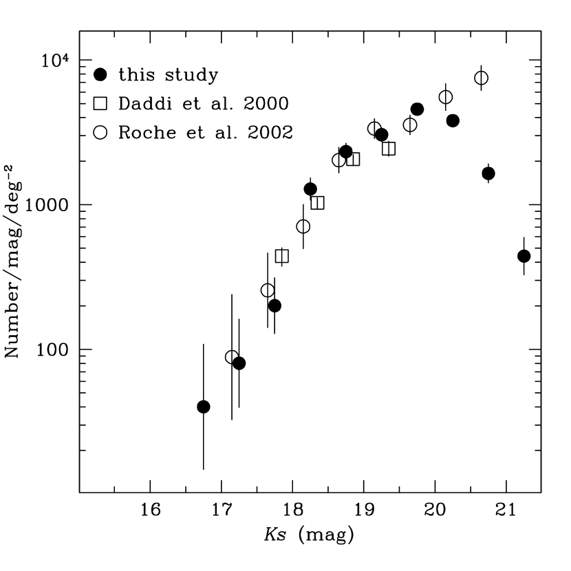
Figure 2.— $Ks$-band differential galaxy counts for the $I-K>4$ mag EROs in the SofI $Ks$-band survey of the PDS (filled circles). Also shown are the $Ks$-band ERO counts from Daddi et al. (2000; squares) and Roche et al. (2002; open circles) offset for clarity by $+0.1$ and $-0.1$ mag respectively. Our sample is complete to $Ks\approx 20$ mag.

3. Two point correlation function of EROs

The two-point angular correlation function, $w(\theta)$, is defined as the joint probability $\delta P$ of finding sources within the solid angle elements $\delta\Omega_{1}$ and $\delta\Omega_{2}$, separated by an angle $\theta$, in the form

$$\delta P=N^{2}\,(1+w(\theta))\delta\Omega_{1}\delta\Omega_{2},$$ (1)

where $N$ is the mean surface density of galaxies. For a random distribution of sources $w(\theta)$=0. Therefore, the angular correlation function provides a measure of galaxy density excess over that expected for a random distribution. Various methods for estimating $w(\theta)$ have been introduced, as discussed by Infante (1994). In the present study, a source is taken as the ‘centre’ and the number of pairs within annular rings is counted. To account for the edge effects, Monte Carlo techniques are used by placing random points within the area of the survey. We use the $w(\theta)$ estimator introduced by Landy & Szalay (1993)

$$w(\theta)=\frac{DD-2DR+RR}{RR},$$ (2)

where DD and DR are respectively the number of sources and random points at separations $\theta$ and $\theta+d\theta$ from a given galaxy. Similarly, RR is the number of random points within the angular interval $\theta$ to $\theta+d\theta$ from a given random point.

For a given ERO sample, a total of 100 random catalogues are generated, each having the same number of points as the original data set. The random sets were cross-correlated with the galaxy catalogue, giving an average value for $w(\theta)$ at each angular separation. The uncertainty in $w$($\theta$) is determined from the relation

$$\sigma_{w}=\sqrt{\frac{1+w(\theta)}{DD}}.$$ (3)

Finally, before fitting a power law to $w(\theta)$, we take into account a bias arising from the finite boundary of the sample. Since the angular correlation function is calculated within a region of solid angle $\Omega$, the background projected density of sources, at a given magnitude limit, is effectively $N_{s}/\Omega$ (where $N_{s}$ is the number of sources brighter than the limiting magnitude). However, this is an overestimation of the true underlying mean surface density, because of the positive correlation between galaxies in small separations, balanced by negative values of $w(\theta)$ at larger separations. This bias, known as the integral constraint, has the effect of reducing the amplitude of the correlation function by

$$\omega_{\Omega}=\frac{1}{\Omega^{2}}\int{\int{w(\theta)d\Omega_{1}d\Omega_{2}}},$$ (4)

where $\Omega$ is the solid angle of the survey area. Following Roche et al. (2002) we estimate $\omega_{\Omega}$ numerically using the random-random correlation

$$\omega_{\Omega}=\frac{\sum{RR\,A_{w}\,\theta^{-\delta}}}{\sum{RR}},$$ (5)

where we assume that $w(\theta)$ is a power-law of the form $A_{w}\,\theta^{-\delta}$. The sum in equation 5 is from 1 arsec to 15 arcmin. Adopting $\delta=0.8$ we find $\omega_{\Omega}=6.9\times A_{w}$. Having fixed the exponent $\delta$ to 0.8 the amplitude $A_{w}$ is obtained by fitting the function $A_{w}\theta^{-0.8}-\omega_{\Omega}$ to the observed $w(\theta)$ using standard $\chi^{2}$ minimisation procedures weighting each point with its error. We estimate the $w(\theta)$ and determine the amplitude $A_{w}$ for different $Ks$-band magnitude limited ERO subsamples. The results are summarised in Table 1. The estimated correlation function is plotted in Figure 3. For the $Ks<19$ and $<19.5$ mag sub-samples the correlation function signal is significant at the $2\sigma$ level with $w(\theta<25^{\prime\prime})=0.68\pm 0.30$ and $0.28\pm 0.13$ respectively. For the sub-sample with $Ks<20$ mag the detected signal is significant at the $3.7\sigma$ confidence level ($w(\theta<25^{\prime\prime})=0.37\pm 0.10$). The amplitudes estimated above must be corrected for contamination of the galaxy sample by stars at faint magnitudes ($Ks>16.5$ mag). The presence of an uncorrelated population of uniformly distributed stars within the galaxy catalogue, reduces $A_{w}$ by the factor

$$\biggl{(}\frac{N_{obj}}{N_{obj}-N_{s}}\biggr{)}^{2},$$ (6)

where $N_{obj}$ is the number of objects (both stars and galaxies) used to calculate $w(\theta)$ and $N_{s}$ is the number of stars in the catalogue. In the present study, stars were identified and removed to $K=16.5$ mag (section 2.2). At fainter magnitudes, the Milky Way stellar population synthesis model described by Robin et al. (2003, 2004) was employed to predict the expected number of stars within our ERO sample at different $Ks$-band magnitude limits. The correction factors estimated from equation 6 are also listed Table 1 along with the corrected amplitudes, $A_{w}^{s}$. The $A_{w}^{s}$ (with $\theta$ measured in degrees) are consistent with previous studies at similar magnitude limits (e.g. Daddi et al. 2001; Roche et al. 2002, 2003). This is demonstrated in Figure 4 plotting the $A_{w}^{s}$ for EROs as a function of the limiting $Ks$-band magnitude. Compared to previous ERO surveys to $Ks=20$ mag our sample has the advantage of larger size and hence more statistically reliable results. Cosmic variance however, is likely to be an issue for surveys with areal extent similar to our own. Daddi et al. (2001) estimated that the relative dispersion on the amplitude of the angular correlation function due to this effect is $\sigma_{A_{w}}/A_{w}=\sqrt{A_{w}\,\,\omega_{\Omega}}$, where $\omega_{\Omega}$ is the integral constraint defined in equation 4. For our survey geometry using this relation we estimate an uncertainty to the amplitudes listed in Table 1 due to cosmic variance of $\approx 20\%$. We note however, that this result is likely to be a lower limit since it does not take into account the higher order moments of the galaxy distribution. For example Barger et al. (1999) and McCracker et al. (2000) find a factor of three difference in the surface density of EROs to $K\approx 20$ mag in their independent small area surveys ($\rm\approx 60\,arcmin^{2}$). Although our sample has 3 times larger field of view the result above illustrates the effect of cosmic variance to relatively small area surveys. Much larger, degree scale, $K$-band samples will be able to address this issue (e.g. NOAO Deep Wide Survey; Brown et al. 2003). N-body simulations can also be used in principle to provide a realistic estimate of the cosmic variance effect (e.g. Somerville et al. 2004). This calculation however, requires a number of assumptions on the redshift distribution and clustering properties of EROs and is beyond the scope of this paper.

We also attempt to quantify the effect of the $Ks$-band catalogue incompleteness at faint magnitudes (20-30% in the range 19.6-20 mag) to the estimated $w(\theta)$ of EROs. We need a sample that does not suffer from incompleteness in the above magnitude range to create mock catalogues by randomly removing 20-30% of the sources at faint magnitudes. The angular correlation function for each mock catalogue is then estimated to quantify the bias introduced by the $Ks$-band catalogue incompleteness. The above prescription could have been applied to the central $\rm 4.5\times 4.5\,arcmin^{2}$ subregion of our survey which is deeper in the $Ks$-band ($Ks\approx 20.5$ mag) and thus does not suffer from incompleteness in the 19.6-20 mag range. However, only about 30 EROs lie in this subregion and therefore the small number statistics do not allow us to use this sample. Nevertheless, we apply the above method to the $Ks<19.5$ mag subsample (total of 177 sources, see Table 1) by randomly removing 20-30% of the sources in the range 19.0-19.5 mag. A total of 500 mock catalogues are created and the amplitude of the angular correlation function of each one of them is estimated. Within the $1\sigma$ uncertainties we find no difference between the mean $A_{w}$ from the 500 mock realisations and that quoted in Table 1. Extrapolating the above result to the $Ks<20$ mag we argue that the estimated amplitude is not going to be significantly affected by incompleteness at faint magnitudes. We caution the reader however, that the above conclusion holds only if the missed objects have the same clustering properties as the detected sources.

The agreement between the angular correlation amplitudes estimated here and those found in previous studies also implies an agreement on the spatial correlation length $r_{o}$ assuming a similar redshift distribution, which is not unreasonable given the similarity of the sample selection. Use of the luminosity function models of Daddi et al. (2001) and Roche et al. (2002, 2003) to deproject the ERO angular correlation amplitudes and to determine their spatial correlation length, $r_{o}$, yields $r_{o}=12-17\,h^{-1}\rm\,Mpc$. The range in $r_{o}$ depends on the adopted luminosity function and clustering evolution model. As discussed above the uncertainty in $r_{o}$ due to cosmic variance is estimated to be at least $\approx 20\%$. We also caution the reader that the relatively small extent of our survey may result in systematic underestimation of the derived correlation length. For example, Daddi et al. (2001) estimate this effect to be $<10\%$.

Table 1 Clustering amplitudes of the $I-K>\rm 4\,mag$ EROs at different magnitude limits. The $A_{w}$ is estimated at 1 degree and is not corrected for dilution due to stellar contamination of the ERO sample at faint magnitudes. The correction factors in the last column account for this effect providing an estimate of the reduction of the measured $A_{w}$ due to the presence of stars (see text for details). The last column gives the clustering amplitudes, $A^{s}_{w}$, corrected for stellar contamination

$Ks$-band	Number of	$A_{w}$	correction	$A^{s}_{w}$
limit (mag)	EROs	($\times 10^{-3}$)	factor	($\times 10^{-3}$)
19.0	100	$7.7^{+5.6}_{-3.3}$	1.52	$11.7^{+8.5}_{-5.0}$
19.5	177	$7.1^{+2.6}_{-2.0}$	1.34	$9.5^{+3.5}_{-2.7}$
20.0	289	$6.8^{+1.6}_{-1.3}$	1.28	$8.7^{+2.1}_{-1.7}$

Figure 3.— Angular correlation function $w(\theta)$ for the three magnitude limited subsamples listed in Table 1. The lines are the best fit to the observations.

Figure 4.— The amplitude of the angular correlation function of EROs as a function of the limiting $Ks$-band magnitude. The filled circles are the results from this study, after applying the correction for stellar contamination, the squares and the open circles are the amplitudes from Daddi et al. (2000) and Roche et al. (2002) respectively.

4. The environment of EROs

In this section we study the environment of EROs to explore their association with regions of enhanced density at relatively high redshifts ($z\approx 1$). We quantify this by cross-correlating the positions of our ERO sample with the smoothed $Ks$-band galaxy density map produced using the matched filter algorithm described by Postman et al. (1996).

4.1. Creating the density map

The matched filter algorithm was developed by Postman et al. (1996) to identify galaxy overdensities using photometric data only. It has the advantage that it exploits both positional and photometric information producing galaxy density maps where spurious galaxy fluctuations are suppressed. A drawback of the matched filter method is that one must assume a form for the cluster luminosity function and its radial profile. Clusters with the same richness but different intrinsic shape or different luminosity function from the adopted ones do not have the same likelihood of being detected.

A detailed description of the matched filter algorithm can be found in Postman et al. (1996). In brief, the galaxy catalogue is convolved with a filter derived from an approximate maximum likelihood estimator obtained from a model of the spatial and luminosity distribution of galaxies within a cluster. The luminosity weighting function (i.e. flux filter) is defined as

$$L(m)=\frac{\phi(m-m^{*})\,10^{-0.4\,(m-m^{*})}}{b(m)},$$ (7)

where $\phi(m-m^{*})$ is the cluster luminosity function, $m^{*}$ is the apparent magnitude corresponding to the characteristic luminosity of the cluster luminosity function and $b(m)$ is the surface density of field galaxies with apparent magnitude $m$. We adopt a Schechter form for the cluster $Ks$-band luminosity function with parameters $\alpha=-1.09$ and $M^{*}=-23.53+5{\rm log}h$ estimated by Kochanek et al. (2001) for early type galaxies. The term $10^{-0.4\,(m-m^{*})}$ in equation 7 is introduced to avoid divergence of the integral of $L(m)$ at faint magnitudes in the case of Schechter luminosity functions with $\alpha<-1$. The spatial weighting function (i.e. radial filter) is assumed to follow the form

$$P(r)=\left\{\begin{array}[]{cc}\frac{1}{\sqrt{1+(r/r_{c})^{2}}}-\frac{1}{\sqrt{1+(r_{co}/r_{c})^{2}}},&\mathrm{if\,\,\,r<r_{co}}\\ 0&\mathrm{otherwise,}\\ \end{array}\right.$$

where $r_{c}$ is the cluster core radius and $r_{co}$ is an arbitrary cutoff radius. Here, we adopt $r_{c}=100\,h^{-1}$ kpc and $r_{co}=1\,h^{-1}$ Mpc (e.g. Postman et al. 1996). In practice the survey area is binned into pixels $(i,j)$ of fixed size (for the choice of values see below) and the observed galaxy distribution is convolved with the filters above producing a likelihood map according to the relation

$$S(i,j)=\sum_{k=1}^{N_{T}}\,P(r_{k})\,L(m_{k}),$$ (8)

where $N_{T}$ is the total number of galaxies in the catalogue. The sum above is evaluated for every pixel of the density map. Both $m^{*}$ and $r_{c}$ are a function of redshift and hence $S(i,j)$ also depends on redshift through these parameters. The redshift dependence of $m^{*}$ also includes a $k$-correction. Here we adopt a non-evolving elliptical galaxy model obtained from the Bruzual & Charlot (1993) stellar population synthesis code as described in Pozzeti, Bruzual & Zamorani (1996).

We apply the matched filter algorithm to galaxies brighter than $Ks=20$ mag in our $Ks$-band survey to avoid biases due to incompleteness at fainter magnitudes. The galaxy density map $S(i,j)$ is independently estimated for redshifts between $z_{min}=0.5$ to $z_{max}=1.2$, incremented in steps of 0.1. The $z_{max}$ corresponds to the redshift where $m^{*}$ becomes comparable to the limiting magnitude of the survey. The characteristic luminosity, $L^{*}$, the faint end slope of the luminosity function, $\alpha$, and the cluster core radius, $r_{c}$, are assumed to remain constant with redshift. Adopting a passively evolving $L^{*}$ for the luminosity function does not alter our main conclusions but, as discussed below, only shifts $z_{max}$ to higher redshifts, $z_{max}\approx 1.6$. For the passive evolution we adopt the elliptical galaxy model described by Pozzeti, Bruzual & Zamorani (1996) which predicts a brightening of $M^{*}$ by about 0.8 magnitudes to $z\approx 1$. This is in fair agreement with recent studies on the $K$-band luminosity function evolution (Pozzetti et al. 2003; Toft et al. 2004; Ellis & Jones 2004). The results presented here assume a constant $L^{*}$ with redshift. The pixel size of the galaxy density maps at any redshift is taken to be $\approx 18$ arcsec corresponding to a projected cluster core radius of $r_{c}=100\,h^{-1}$ kpc at the redshift $z=1$. Figure 5 shows the $z=1.1$ density map generated by the method above with the positions of EROs overplotted.

Figure 5.— $Ks$-band density map with parameters tuned to $z=1.1$. The contours delineate the regions with overdensity $>1$ (i.e. above the mean density of the map). The circles show the positions of $Ks<20$ mag EROs in our sample.

4.2. ERO/density-map cross-correlation

The cross-correlation function between the $Ks<20$ mag EROs and the $Ks$-band density map (at a given redshift) is estimated using the relation

$$w_{E,D}(\theta)=\frac{1}{N_{eros}}\,\sum_{k}^{N_{eros}}\sum_{i,j}(S_{i,j}-\bar{S}),$$ (9)

where $N_{eros}$ is the total number of EROs, $S_{i,j}$ is the value of the $(i,j)$ pixel of the density map produced using the prescription described in the previous section, $\bar{S}$ is the mean value of the density map and the sum is for all pixels with angular separation $\theta$ from a given ERO. The uncertainties were estimated from 100 bootstrap resamples of the EROs. Simulated data sets were generated by sampling N points with replacement from the true ERO dataset of N points. The cross-correlation function is then estimated for each of the bootstrap samples in the same fashion as with the real dataset. The standard deviation around the mean for a given angular separation $\theta$ is the used to estimate the uncertainty in the $w_{E,D}(\theta)$.

To assess the expectation in the case of a random distribution of points we produce 100 mock $Ks$-band catalogues by randomising the positions of the $Ks$-band galaxies. We then apply the matched filter algorithm to produce density maps for each of the independent mock catalogues. The (randomised) positions of the EROs in the mock catalogues are then cross-correlated with the density maps in the same fashion as for the real dataset. For each separation $\theta$ the above procedure provides an estimate of the cross-correlation function expected in the case of a random distribution of galaxies (i.e. without clustering). This procedure also takes into account the presence of spurious galaxy overdensities that may be produced by the matched filter algorithm.

Using the procedure above we cross-correlate the $Ks<20$ mag EROs with the density maps produced by the matched filter algorithm with parameters tuned at redshifts $z=0.5-1.2$. The results for the $z=0.7$, 0.9 and 1.1 density maps are plotted in Figure 6 along with the random expectation. There is evidence for a statistically significant ($\approx 3\sigma$) positive signal for angular separations 0–60 arcsec in the case of the high redshift density maps (e.g. $z=0.9$, 1.1). At lower redshifts (e.g. $z=0.7$) we find no signal above the random expectation. This is further demonstrated in Figure 7 plotting the significance above the random expectation of the detected $w_{E,D}(\theta)$ signal for separations 0–60 arcsec (i.e. the first bin in Figure 6) as a function of the redshift that the density map was estimated. The significance in this figure is expressed in units of standard deviations, $\sigma$, taking into account the uncertainties in both the $w_{E,D}(\theta)$ and the random expectation. In Figure 7 the significance of the $w_{E,D}(\theta)$ signal increases with redshift to about $3\sigma$ when the cross-correlation is performed with density maps generated for redshifts $z\gtrsim 1$. Adopting a passively evolving $L^{*}$ for the luminosity function (see section 4.1) shifts the curve in Figure 7 to higher redshifts with the peak at $z=1.2$ moving to $z=1.6$ but does not qualitatively alter the results. This is demonstrated in the insert plot of Figure 7. The evidence above suggests that EROs are associated with high-$z$ overdensities.

We also explore if non-ERO (i.e. $I-K<4$) $Ks$-band selected galaxies with the same magnitude distribution as the ERO sample give equally significant cross-correlation signal. We produce a total of 100 mock catalogues by randomly selecting galaxies from the full $Ks$-band source list with $I-K<4$ (i.e. not EROs) and magnitude distribution similar to that of our $Ks<20$ mag ERO sample. Each of these mock catalogues are cross-correlated with the $Ks$-band density maps providing, at different redshifts, an estimate of the mean cross-correlation function and its rms for each separation. This is then compared against the signal for EROs. For the $z=1.2$ and $1.1$ maps we find that the ERO signal is higher than that of non-ERO galaxies, on average, at the $2.6\sigma$ and $2.1\sigma$ confidence level respectively. For lower redshifts the EROs have cross-correlation signal consistent with that of non-EROs within the $1\sigma$ uncertainties. This is demonstrated in Figure 7 plotting the significance above the random expectation of the mean $w_{E,D}(\theta)$ signal for non-ERO $Ks$-band selected galaxies for separations 0–60 arcsec as a function of the redshift that the density map was estimated. Together this all provides direct evidence that EROs are associated with regions of enhanced density at $z\gtrsim 1$.

Figure 6.— Cross-correlation function $w_{E,D}(\theta)$ of the $Ks<20$ mag EROs and the density map produced by the matched filter algorithm of Postman et al. (1996) at redshifts $z=0.7$, 0.9 and 1.1. The continuous line is the expectation for a random distribution of galaxies and the dashed lines are the $1\sigma$ uncertainty envelop around the mean.

Figure 7.— Significance above the random expectation of the detected $w_{E,D}(\theta)$ signal for separations 0–60 arcsec as a function of the redshift that the density map (used in the cross-correlation) was estimated assuming an non-evolving $L_{*}$. The filled circles are the $Ks<20$ mag ERO sample ($I-K>4$ mag) and the open squares are non-ERO (i.e. $I-K<4$) $Ks$-band selected galaxies (see text for details). The significance is in standard deviations, $\sigma$, taking into account the uncertainties in both the $w_{E,D}(\theta)$ and the random expectation. The insert plot shows the same results ($w_{E,D}(\theta)$ significance versus $z$) in the case of density maps estimated assuming passively evolving $L_{*}$ luminosity. There is no qualitative difference between the non-evolving and passively evolving $L_{*}$ results except from the $z_{max}$ which shifts from 1.2 to 1.6 in latter case.

5. EROs and the faint radio population

Radio galaxies are another class of sources that are believed to be good cluster tracers to high-$z$ (e.g. Zirbel 1997; Zanichelli et al. 2001). We exploit the deep 1.4 GHz radio observations available for our $Ks$-band survey to explore the association of EROs with radio sources and whether they trace similar structures. These are quantified using the two-point cross-correlation function $w_{1.4,E}(\theta)$ between radio sources and EROs.

The cross-correlation function is estimated taking radio sources as centres and counting the number of EROs around them in successive annuli. This is then compared with the expectation for a random distribution by placing a total of 40 000 random points in the surveyed area and counting the number of pairs between radio sources and the random points. The cross-correlation function is defined

$$w_{1.4,E}(\theta)=\frac{DD(1.4,E)\,\,N_{R}}{DR(1.4,R)\,\,N_{E}}-1,$$ (10)

where $DD(1.4,E)$, $DR(1.4,R)$ is the number of radio/ERO and radio/random pairs respectively with separation $\theta$ and $N_{R}$, $N_{E}$ is the total number of random points and EROs respectively. As already discussed, in the cross-correlation we have excluded a total of 17 radio sources that are associated with EROs. The results for the remaining 78 radio sources in our sample are plotted in the bottom panel of Figure 8 with the errors being Poisson estimates. There is little signal with the estimated $w_{1.4,E}(\theta)$ consistent with zero. This suggests that the bulk of the EROs and the radio source populations are probing different structures.

We further explore this by grouping the radio sources into high and low-$z$ sub-samples using the photometric redshift estimates presented by Sullivan et al. (2004). The low-$z$ sub-sample comprises 35 sources with $z_{phot}<0.6$ while, the high-$z$ sub-sample includes a total of 43 sources both without optical counterparts to the limit $I\approx 24$ mag (assumed to lie at high redshifts) and with $z_{phot}>0.6$. The cross-correlation results using the above sub-samples are plotted in the middle (low-$z$) and top panels (high-$z$) of Figure 8. Although there is no signal in the case of the low-$z$ radio sources, the high-$z$ sub-sample shows signal for separations 7–30 arcsec, albeit at the $\approx 2\sigma$ significance level ($w_{1.4,E}(7-30^{\prime\prime})=0.34\pm 0.18$). Although the statistics are poor the evidence above suggests that the different redshift distributions of the radio and ERO populations are responsible for the lack of cross-correlation signal in the bottom panel of Figure 8. The EROs peak at $z\gtrsim 1$ (e.g. Cimatti et al. 2001, 2003; Firth et al. 2002; Väisänen & Johansson 2004a) while many of the radio sources to the flux density limit of the PDS lie at $z\lesssim 1$ (Georgakakis et al. 1999; Afonso et al. 2004; Sullivan et al. 2004).

This is also supported by the cross-correlation of the full radio sample with the $Ks$-band density maps produced in section 4.1. The cross-correlation is performed using the method outlined in section 4.2. The expectation in the case of a random distribution of points is quantified by producing 100 mock radio catalogues by randomising the positions of the radio sources. Each of these random catalogues is cross-correlated with the $Ks$-band density maps providing, for a given separation $\theta$, an estimate of the cross-correlation function expected in the case of a random distribution of galaxies (i.e. without clustering).

The results are shown in Figure 9 plotting the significance above the random expectation of the detected cross-correlation signal for separations 0–60 arcsec as a function of the redshift that the density map was estimated (assuming a non-evolving $L^{*}$). The significance in this figure is expressed in units of standard deviations, $\sigma$. In Figure 9 the significance of the cross-correlation signal decreases with redshift falling below the $\approx 3\sigma$ when the cross-correlation is performed with density maps generated for redshifts $z>0.7$. Adopting a passively evolving $L^{*}$ for the luminosity function (see section 4.1) does not qualitatively change our results but only shifts to higher-$z$ the point that the significance of the cross-correlation signal falls below $\approx 3\sigma$. This is demonstrated in the insert plot of Figure 9.

The trend for radio sources in Figure 9 is opposite to that for EROs in Figure 7 suggesting that the bulk of the radio and the ERO populations are tracing structures at different redshifts.

Figure 8.— Cross-correlation function $w_{1.4,E}(\theta)$ of the faint radio sources with the $Ks<20$ mag EROs. The dashed lines in all panels mark the expectation for a random distribution. The bottom panel is the $w_{1.4,E}(\theta)$ using the full sample (78) of faint radio sources. The middle panel is the cross-correlation function using the low-$z$ sub-sample with photometric redshift estimates $z<0.6$. The top panel is for the faint radio source sub-sample with photometric redshifts $z>0.6$ or no optical counterparts.

Figure 9.— Significance above the random expectation of the cross-correlation function, $w_{1.4,D}(\theta)$, between the faint radio sources and the $Ks$-band density maps at different redshifts produced as described in section 4. The density maps are estimated assuming a non-evolving $L_{*}$ for the luminosity function. We plot the $w_{1.4,D}(\theta)$ signal for separations 0–60 arcsec expressed in standard deviations, $\sigma$, taking into account the uncertainties in both the $w_{1.4,D}(\theta)$ and the random expectation.The insert plot shows the same results ($w_{1.4,D}(\theta)$ significance versus $z$) in the case of density maps estimated assuming passively evolving $L_{*}$ luminosity. There is no qualitative difference between the non-evolving and passively evolving $L_{*}$ results.

6. Discussion and summary

In this paper we explore the clustering properties of $Ks<20$ mag EROs ($I-K>4$ mag) using a $Ks$-band sample covering $\rm\approx 180\,arcmin^{2}$ and overlapping with the PDS region. We use angular correlation function analysis to estimate a statistically significant clustering signal ($>3\sigma$) with amplitude consistent, within the errors, with previous studies (Roche et al. 2002, 2003; Daddi et al. 2000). The advantage of our study is that our sample size is larger than previous surveys to $Ks=20$ mag (e.g. Roche et al. 2002, 2003) providing better statistical reliability. Nevertheless, cosmic variance remains an issue in our survey. The $w(\theta)$ amplitudes estimated here are consistent with 3-D clustering lengths $r_{o}=\rm 12-17\,h^{-1}\,Mpc$ depending on the adopted model luminosity function and the evolution of the clustering (Daddi et al. 2001; Roche et al. 2002, 2003). These $r_{o}$ values are in-between those of present-day ellipticals (e.g. Guzzo et al. 1997) and Abell clusters (Abadi, Lambas & Muriel 1998) and comparable to those estimated for hard X-ray selected sources (Basilakos et al. 2004) and SCUBA sources (Almaini et al. 2003). Daddi et al. (2002) also discuss evidence that EROs with optical/NIR colours suggesting old stellar population are significantly more clustered than those showing evidence for dusty starbursts.

A number of studies also suggest a dependence of the correlation length on the galaxy absolute luminosity (e.g. Willmer, da Costa & Pellegrini 1998; Norberg et al. 2002; Zehavi 2002; Brown et al. 2003). For example, Brown et al. (2003) estimated the correlation length of $z<1$ red ($B_{W}-R>1.44$) galaxies in the NOAO Deep Wide Field Survey and found that systems with $L>L^{*}$ have higher clustering lengths ($r_{o}\approx 10\,h^{-1}\rm\,Mpc$) than $<L^{*}$ galaxies ($r_{o}\approx 5\,h^{-1}\rm\,Mpc$). Similar results are obtained for the early type galaxies in the 2dF Galaxy Redshit Survey (Norberg et al. 2002). The EROs identified in our sample comprise systems with $L\lesssim L^{*}$. For example at $z=1$ and 1.5 the magnitude limit $Ks=20$ mag corresponds to about $0.2\,L^{*}$ and $0.5\,L^{*}$ respectively, assuming a passively evolving elliptical galaxy model. The large clustering lengths of $Ks\approx 20$ mag EROs ($r_{o}=12-17\,h^{-1}\rm\,Mpc$) are therefore difficult to reconcile with the above $r_{o}$ estimates for $L\lesssim L^{*}$ early type galaxies at $z<1$. This may be due to uncertainties in the model redshift distribution of EROs used to deproject the angular correlation function amplitudes. Combination of photometric and spectroscopic redshifts for complete ERO samples are essential to refine these models and to better understand the clustering properties of this population.

The evidence above on the large correlation length of EROs may suggest these sources are tracing high density regions. We further explore the association of EROs with galaxy overdensities using a novel method: we first smooth the $Ks$-band galaxy distribution using the matched filter algorithm of Postman et al. (1996) and then cross-correlate the resulting density maps with the ERO positions. The matched filter algorithm parameters are tuned to produce density maps each one of which is sensitive to galaxy clusters at a different redshift in the range 0.5–1.2. We find a statistically significant cross-correlation signal ($\gtrsim 3\sigma$ compared to the random distribution) only for density maps tuned to $z\gtrsim 1$ clusters. At these redshifts, EROs also have higher cross-correlation signal, albeit at the $2-2.5\sigma$ confidence level, than the non-ERO $Ks$-band selected galaxies with the same magnitude distribution. This provides direct evidence that EROs are, on average, associated with regions of enhanced galaxy density at redshifts $z\gtrsim 1$. Previous studies also claim that EROs lie within rich cluster regions at high-$z$. Daddi et al. (2000) and Roche et al. (2002) have identified ERO overdensities within their surveys and argued that these may be associated with massive clusters at $z\gtrsim 1$. Väisänen & Johansson (2004b) also report overdesnities of EROs in the vicinity of faint mid-IR ISO sources and argue that these may be associated with high-$z$ clusters. Similar enhanced ERO number densities have been reported in high-$z$ AGN and QSO fields (e.g. McCarthy, Presson & West 1992; Hu & Ridgeway 1994; Chapman, McCarthy & Persson 2000; Hall et al. 2001; Best et al. 2003; Wold et al. 2003), although is not yet clear if these ERO overdensities are indeed associated with clusters linked to the central AGN. Our analysis provides direct evidence that EROs are associated with high-$z$ overdense regions and confirms the claims of the studies above.

Also, our finding that EROs trace dense regions at $z\gtrsim 1$ is consistent with previous studies on the redshift distribution of EROs. The red $I-K$ colours of these systems can only be explained by either early type galaxies or dusty starbursts at $z\gtrsim 0.8$ (e.g. Pozzetti & Mannucci 2000; Väisänene & Johansson 2004a; Roche et al. 2002, 2003). Luminosity function models used to interpret the observed ERO counts and their clustering properties produce spiky redshift distributions with a peak at $z\approx 1$ and a long tail extending to high-$z$ (Daddi et al. 2001; Roche et al. 2003). Spectroscopic and photometric redshifts for EROs also show that most of them are associated with $z\gtrsim 1$ ellipticals or dusty starbursts, although the relative mix of the two populations remain poorly constrained (e.g. Cimatti et al. 1998; Dey 1999; Piere et al. 2001; Smith et al. 2001; Afonso et al. 2001; Cimatti et al. 2001; Daddi et al. 2003; Martini 2001).

We also investigate the association between EROs and faint radio sources and how they trace large scale structures by exploiting the deep radio data available for $Ks$-band survey. We find that only a small fraction of $Ks<20$ mag EROs have radio counterparts to the $\rm 60\mu Jy$ limit of the radio data (17 out of 289). This is much lower than the identification fraction reported by Smail et al. (2002; 21/68) and Roche et al. (2003; 7/31) which is attributed to the deeper radio observations in those studies. Indeed, Smail et al. (2002) find that the number of EROs detected at radio wavelengths rapidly increases at faint flux densities, doubling below $\approx\rm 40\mu Jy$. Using stacking analysis we estimate a mean radio flux density for EROs of $\approx 8\,\mu$Jy, about 1 dex lower than the limit of our survey. Much deeper observations are therefore required to identify the bulk of the radio counterparts for EROs.

Cross-correlating the radio and ERO positions (after excluding the 17 EROs with 1.4 GHz emission) does not produce any signal, suggesting little association between the two populations. However, for the sub-sample of radio sources with photometric redshifts $z>0.6$ or no optical counterparts (assumed to lie at high-$z$) we get a marginally significant signal at the $\approx 2\sigma$ level. Although the small number statistics (only 43 radio sources fulfilling the above criteria) hamper a secure interpretation, the evidence above suggests that it is the high-$z$ radio population that appears to trace similar large scale structures with EROs.

A large fraction of the radio population however, to the limit of our survey, is associated with moderate and low-$z$ starburst systems (Georgakakis et al. 1999; Afonso et al. 2004) tracing structures at $z<1$. Cross-correlation of the full radio sample with the $Ks$-band density maps gives a statistical significant signal ($\gtrsim 3\sigma$) only at $z\lesssim 0.7$, contrary to the ERO population with a cross-correlation signal that peaks at $z\gtrsim 1$. This explains why cross-correlation of the full radio and ERO samples does not produces a statistically significant signal.

Summarising our conclusions:

• using angular correlation function analysis we estimate a statistically significant signal ($>3\sigma$) for $Ks<20$ mag EROs. The derived correlation function amplitude is consistent with previous studies that used smaller sample sizes. This amplitude translates to clustering lengths in the range $r_{o}=12-17\,h^{-1}\rm\,Mpc$.

• cross-correlation of the ERO positions with the $Ks$-band density maps gives a statistically significant signal only for the $z\gtrsim 1$ maps. This cross-correlation signal is higher, albeit at the $2-2.5\sigma$ level, from that obtained for non-ERO galaxies with the same magnitude distribution as our ERO sample. We argue that this is direct evidence that EROs are associated with regions of enhanced density at redshifts $z>1$.

• 17 of the 289 EROs with $K<20$ mag show radio emission with flux densities in the range $\rm 65-1000\mu Jy$. Using stacking analysis we estimate a mean radio flux density of $\approx\rm 8\,\mu$Jy for EROs.

• cross-correlation of the radio and the ERO samples (after excluding the 17 EROs with radio counterparts) gives a $2\sigma$ signal only for the sub-sample of high-$z$ radio sources ($z\gtrsim 0.6$). Although the statistics are poor this suggests that the bulk of the radio and the ERO populations trace different structures. Indeed, cross-correlation of the radio positions with the $Ks$-band density maps gives a statistically significant signal only for the $z\lesssim 0.7$ maps, contrary to EROs.

7. Acknowledgments

We thank the anonymous referee for useful comments and suggestions. AG acknowledges funding by the European Union and the Greek Ministry of Development in the framework of the Programme ’Competitiveness- Promotion of Excellence in Technological Development and Research- Action 3.3.1’, Project ’X-ray Astrophysics with ESA’s mission XMM’, MIS-64564. AMH acknowledges support provided by the National Aeronautics and Space Administration through Hubble Fellowship grant HST-HF-01140.01-A awarded by the Space Telescope Science Institute. JA gratefully acknowledges the support from the Science and Technology Foundation (FCT, Portugal) through the fellowship BPD-5535-2001 and the research grant POCTI-FNU-43805-2001. The Phoenix Deep Survey radio data are electronically available at http://www.atnf.csiro.au/people/ahopkins/phoenix/.

References

- (1) Abadi M., Lambas D., Muriel H., 1998, ApJ, 507, 526
- (2) Afonso J., Mobasher B., Chan B., Cram L., 2001, ApJ, 559, L101
- (3) Afonso J., Georgakakis A., Hopkins A., Sullivan M., Mobasher B., Cram L. E., 2004, ApJS, submitted
- (4) Almaini et al., 2003, MNRAS, 338, 303
- (5) Barger A. J. et al., 1999, AJ, 117, 102
- (6) Basilakos S., Georgakakis A., Plionis M., Georgantopoulos I., 2004, ApJ, 607, L79
- (7) Baugh C. M., Cole S., Frenk C. S., 1996, MNRAS, 283, 1361
- (8) Bell E. F., 2003, ApJ, 586, 794B
- (9) Bertin E. & Arnouts S., 1996, A&AS, 117, 393
- (10) Best P. N., Lehnert M. D., Miley G. K., Röttgering H. J. A., 2003, MNRAS, 343, 1
- (11) Brown M. J. I., Dey A., Jannuzi B. T., Lauer T. R., Tiede G. P., Mikles V. J., 2003, ApJ, 597, 225
- (12) Brusa M., Comastri A., Daddi E., Cimatti A., Mignoli M., Pozzetti L., 2002, ApJ, 581L, 89
- (13) Bruzual A. G. & Charlot S., 1993, ApJ, 405, 538
- (14) Chapman S.C., McCarthy P. J., Persson S. E., 2000, AJ, 120, 1612
- (15) Cimatti A., Andreani P., Röttgering H., Tilanus R., 1998, Nature, 392, 895
- (16) Cimatti A. et al., 2002, A&A, 381, L68
- (17) Cimatti A. et al., 2003, A&A., 412, L1
- (18) Daddi E., Cimatti A., Pozzetti L., Hoekstra H., Röttgering H., Renzini A., Zamorani G., Mannucci F., 2000, A&A, 361, 535
- (19) Daddi E. Broadhurst T., Zamorani G., Cimatti A., Röttgering H., Renzini A., 2001, A&A, 376, 825
- (20) Daddi E. et al., 2002, A&A, 384, L1
- (21) Daddi E. et al., 2003, ApJ, 588, 50
- (22) Dey A., Graham J., Ivisob R. J., Smail I., Wright G., Liu M., 1999, ApJ, 519, 610
- (23) Dunlop J., Peacock J., Spinrad H., Dey A., Jimenez R., Stern D., Windhorst R., 1996, Nature, 381, 581
- (24) Eggen O. J., Lynden-Bell D., Sandage A. R., 1962, ApJ, 136, 748
- (25) Ellis S. C., Jones L. R., 2004, MNRAS, 348, 165
- (26) Firth A.E. et al., 2002, MNRAS, 332, 617
- (27) Gardner J. P., Cowie L. L., Wainscoat R. J., 1993, ApJ, 415L, 9
- (28) Georgakakis A., Mobasher B, Cram L., Hopkins A., Lidman C., Rowan-Robinson M., 1999, MNRAS, 306, 708
- (29) Glazebrook K., Peacock J. A., Collins C. A., Miller L., 1994, MNRAS, 266, 65
- (30) Guzzo L., Strauss M., Fisher K., Giovanelli R., Haynes M., ApJ, 542, 37
- (31) Hall P. B. et al., 2001, 121, 1840
- (32) Hopkins A. M., Afonso J., Georgakakis A., Sullivan M., Mobasher B., Cram L. E., 2004, in ”Multiwavelength Cosmology” conference, ed. M. Plionis, pg. 125, astro-ph/0309147
- (33) Hopkins A. M., Afonso J., Chan B., Cram L. E., Georgakakis A., Mobasher B., 2003, AJ, 125, 465
- (34) Hopkins A., Afonso J., Cram L., Mobasher B., 1999, ApJ, 519L, 59
- (35) Hopkins A. M., Mobasher B., Cram L., Rowan-Robinson M., 1998, MNRAS, 296, 839H
- (36) Hu E. M., Ridgway S. E., 1994, AJ, 107, 1303
- (37) Infante L., 1994, A&A, 282, 353
- (38) Kauffmann G., 1996, MNRAS, 281, 487
- (39) Kochaneck C., et al., 2001, ApJ, 560, 566
- (40) Kron R. G., 1980, ApJS, 43, 305
- (41) Landy S. D., Szalay S. A., 1993, ApJ, 412, 64
- (42) Larson R. B., 1975, MNRAS, 173, 671
- (43) Norberg P. et al., 2002, MNRAS, 332, 827
- (44) Martini P., 2001, AJ, 121, 2301
- (45) McCarthy P.J., Persson S. E., West S. C., 1992, ApJ, 386, 52
- (46) McCracken H. J., Metcalfe N., Shanks T., Campos A., Gardner J. P., Fong R., 2000, MNRAS, 311, 707
- (47) Pierre M., et al., 2001, A&A, 372, L45
- (48) Postman M., Lubin L. M., Gunn J. E., Oke J. B., Hoessel J. G., Schneider D. P., Christensen J. A., 1996, AJ, 111, 615
- (49) Pozzeti L., Bruzual A. G., & Zamorani G., 1996, MNRAS, 281, 953
- (50) Pozzetti L., Mannucci F., 2000, MNRAS, 317, 17
- (51) Pozzetti L., et al., 2003, A&A, 402, 837
- (52) Robin A. C., Reylé C., Derriére S., Picaud S., 2003, A&A, 409, 523
- (53) Robin A. C., Reylé C., Derriére S., Picaud S., 2004, A&A, 416, 157
- (54) Roche N., Almaini O., Dunlop J., Ivison R.J., Willott C.J., 2002, MNRAS, 337, 1282
- (55) Roche N., Dunlop J., Almaini O., 2003, MNRAS, 346, 803
- (56) Rodighiero G., Franceschini A., Fasano A., 2001, MNRAS, 324, 491
- (57) Smail I., Owen F. N., Morrison G. E., Keel W. C., Ivison R. J., Lendlow M. J., 2002, ApJ, 581, 844
- (58) Smith G. P., Treu T., Ellis R., Smail I., Kneib J.-P., Frye B. L., 2001, ApJ, 562, 635
- (59) Somerville R. S., Lee K., Ferguson H. C., Gardner J. P., Moustakas L. A., Giavalisco M., 2004, ApJ, 600, 171L
- (60) Spinrad H., Dey A., Stern D., Dunlop J., Peacock J., Jimenez R., Windhorst R. 1997, ApJ, 484, 581
- (61) Stanford S., Elston R., Eisenhardt P., Spinrad H., Stern D., Dey A., 1997, AJ, 114, 2232
- (62) Sullivan M., Hopkins A. M., Afonso J., Georgakakis A., Mobasher B., Cram L. E., 2004, ApJS, in press
- (63) Toft S., Mainieri V., Rosati P., Lidman C., Demarco R., Nonino M., Stanford S. A., 2004, A&A, 422, 29
- (64) Väisänen P. & Johansson P. H., 2004a, A&A, 421, 821
- (65) Väisänen P. & Johansson P. H., 2004b, A&A, 422, 453
- (66) Willmer C. N. A., da Costa L. N., Pellegrini P. S., 1998, AJ, 115, 869
- (67) Wold M., Armus L., Neugebauer G., Jarrett T. H., Lehnert M. D., 2003, AJ, 126, 1776
- (68) Zanichelli A., Scaramella R., Vettolani G., Vigotti M., Bardelli S., Zamorani G., 2001, A&A, 379, 35
- (69) Zehavi I. et al., 2002, ApJ, 571, 172Z
- (70) Zepf S. E., 1997, Nature, 390, 377
- (71) Zirbel E. L., 1997, ApJ, 476, 489