Inferring coronal structure from X-ray lightcurves and Doppler shifts: a Chandra study of AB Doradus.

Abstract

The Chandra X-ray observatory monitored the single cool star, AB Doradus, continuously for a period lasting 88 ksec (1.98 $P_{\rm rot}$) in 2002 December with the LETG/HRC-S. The X-ray lightcurve shows rotational modulation, with three peaks that repeat in two consecutive rotation cycles. These peaks may indicate the presence of compact emitting regions in the quiescent corona. Centroid shifts as a function of phase in the strongest line profile, O viii 18.97 Å, indicate Doppler rotational velocities with a semi-amplitude of $30\pm 10$ $\mbox{km}\,\mbox{s}^{-1}$. By taking these diagnostics into account along with constraints on the rotational broadening of line profiles (provided by archival Chandra HETG Fe XVII and FUSE Fe XVIII profile) we can construct a simple model of the X-ray corona that requires two components. One of these components is responsible for 80% of the X-ray emission, and arises from the pole and/or a homogeneously distributed corona. The second component consists of two or three compact active regions that cause modulation in the lightcurve and contribute to the O viii centroid shifts. These compact regions account for 16% of the emission and are located near the stellar surface with heights of less than 0.3 $\mbox{R}_{*}$. At least one of the compact active regions is located in the partially obscured hemisphere of the inclined star, while one of the other active regions may be located at $40$^∘. High quality X-ray data such as these can test the models of the coronal magnetic field configuration as inferred from magnetic Zeeman Doppler imaging.

1 Introduction

Stellar coronae affect how ZAMS stars spin down, how binary systems interact, and even how planets form. Magnetically driven winds control the spin-down rates of young main sequence low mass stars; the latitudes at which these winds originate affect the time-scale on which the star will spin down (Solanki, Motamen & Keppens 1997). Heating from active coronae also affects planetary atmospheres, e.g. XUV radiation by young active stars significantly affects atmospheric escape rates for surrounding giant exo-planets, potentially causing them to evaporate entirely at close orbital distances (Lammer et al. 2003).

X-ray and EUV observations from the Chandra, XMM-Newton and EUVE satellites have revealed that coronae in active cool stars are unlike anything observed on the Sun (Dupree et al. 1993). Emission measure distributions (EMDs) in even relatively quiescent coronae are different from the Sun, with higher levels of emission ($10^{52}$ cm^-3) and a markedly different shape (with a sharp peak at 8 MK). Furthermore, electron densities are greater than $10^{10}$ cm^-3 in plasma at temperatures of 8 MK and beyond (e.g. Güdel et al. 2001; Sanz-Forcada et al. 2002). To compare, in active regions on the Sun, emission measures peak at about $10^{50}$ cm^-3 at 2.5 MK (Brickhouse, Raymond & Smith 1995; Orlando, Peres & Reale 2000).

While the thermal properties of active stellar coronae are increasingly well-determined, we have yet to establish where the emitting plasma is located relative to the stellar surface. It is difficult to build a detailed picture of coronal structure as active stars are too distant to resolve at X-ray and EUV wavelengths. We therefore have to rely on indirect techniques, only rarely applicable, to evaluate the location and extent of the emitting corona (see review by Schmitt 1998). For example, periodic photometric variations in the EUV flux of the contact binary 44i Boo strongly constrained the location of the emission in a small, dense high-latitude region on the primary star (Brickhouse & Dupree 1998); the long exposure time (covering 19 orbital periods) and relatively low levels of flaring facilitated these measurements. On the other hand, large X-ray flares can dominate the emission, and thus eclipse mapping of flares can also reveal the location of X-ray plasma as the flares originate in localized regions. Flaring loop lengths can be estimated from rise-times and decay time-scales in X-ray lightcurves, assuming a single heating event (Favata et al. 2000). Positions can be determined if the flare is eclipsed by the companion in an eclipsing binary system, e.g. a flare observed in the eclipsing binary, Algol (B8V+K2IV), was completely eclipsed, thus strongly constraining its location to 0.5  $\mbox{R}_{*}$ above the “south” pole of the K star (Schmitt & Favata 1999; Favata & Schmitt 1999). Modelling of X-ray flares in the eclipsing binary, YY Gem (dM1e+dM1e), also indicates the presence of compact flaring loops around one of its components (Güdel et al. 2001, Stelzer et al. 2002).

Spectra from the Chandra and XMM-Newton telescopes are of sufficiently high resolution ($100<R<2500$) that individual spectral line profiles can now be analyzed. Brickhouse et al. (2001) exploited the spectral resolution in a Chandra/HETG dataset of the contact binary, 44i Boo (G2V+G2V) to evaluate the location of the emitting corona. They measured Doppler shifts as a function of orbital phase in the centroids of emission line profiles and found strong evidence for rotational modulation. Taking this into account along with the modulation observed in the X-ray lightcurve of the dataset, they find that the regions causing the velocity variations are located near the pole of the primary star.

AB Doradus (AB Dor, HD36705) is a well-studied example of a single, active K0 dwarf that has recently arrived on the main sequence. It rotates very rapidly ($P_{\rm rot}=0.51479$ day, $v_{e}\,\sin\,i$=90 $\mbox{km}\,\mbox{s}^{-1}$) so two rotation cycles can be covered in just over a day. AB Dor also shows signs of magnetic activity at almost all wavelengths; it shows strong photometric variability due to dark surface spots and is very X-ray luminous, $L_{\rm X}/L_{\rm bol}\approx 10^{-3}$ (Vilhu & Linsky 1987). Its emission measure distribution (EMD) derived using EUVE data is typical for an active cool star, whether an RSCVn binary or a ZAMS star (Sanz-Forcada et al. 2002; Sanz-Forcada et al. 2003). Surface spot maps of AB Dor also show activity patterns typical of active cool stars; with a dark cool polar spot, extending down to about 70^∘ latitude, co-existing with lower latitude spots (e.g. Donati et al. 1999; Unruh, Collier Cameron & Cutispoto 1997). The polar spot is extremely stable with a lifetime of several years, while the lower latitude spots appear to have periods of about one month (Hussain 2002).

An increasing amount of evidence supports the picture of a compact ($<1\,R_{*}$), hot ($>1$ MK) corona in AB Dor: (a) density-sensitive Fe-line ratio measurements from EUVE spectra suggest that the stable 8 MK emission peak in AB Dor’s EMD is associated with high densities, $n_{e}\approx 10^{12}$ cm^-3 that are likely to be associated with strong magnetic fields near its surface (Sanz-Forcada, Brickhouse & Dupree 2002); (b) X-ray and UV lightcurves of AB Dor indicate rotational modulation at the 5–13% level (Kürster et al. 1997; Brandt et al. 2001), suggesting that a component of the corona is inhomogeneously distributed – either very near the surface or else concentrated in compact, mid-to-low latitude regions in the extended corona; (c) a flare observed in AB Dor by BeppoSAX was found to be located $0.3\,R_{*}$ above the surface in the circumpolar region of the star (Maggio et al. 2000). However, there is also evidence of cooler ($8\times 10^{3}<T<10^{5}$ K) magnetically-confined material out to distances between 2–6 $\mbox{R}_{*}$ in several active cool stars including AB Dor and V711 Tau (e.g. Collier Cameron, Jardine & Donati 2002; Walter 2004). Transition region UV line widths (e.g. C iii 1176 Å and O vi 1032 Å) may be significantly large due to rotational broadening (Redfield et al. 2002). It is unclear whether or not this circumstellar material is also associated with hot ($>$ MK) coronal plasma.

We have acquired spectra of AB Dor with the Chandra low energy transmission grating (LETG) covering almost two full rotation cycles. We use Gaussian-fitting routines to measure Doppler shifts in AB Dor’s corona and thus to evaluate the locations of X-ray emitting regions. Details of the Chandra observations and data reduction procedures are outlined in Section 2. In Section 3 we discuss the results from our analysis of the X-ray lightcurve. The LETG spectra are described and analyzed in Section 4. In Section 5 we look for evidence of rotational broadening in LETG and high energy transmission grating (HETG) datasets of AB Dor. Finally, we summarize our main results and use them to derive a simple model of the X-ray emitting corona in Sections 6 and 7.

2 Observations and data reduction

Figure 1: Chandra LETG/HRC-S spectrum integrated over 88.1 ksec (1.98$P_{\rm rot}$). The upper panels show the background-substracted spectra in the short and long wavelength regions. The lower panels show the corresponding background levels. Note that while the spectral resolution in the long wavelength region is better, this region also has fewer counts and a relatively high background level. The lines used in this paper are identified in the figure.

We observed AB Dor using the Chandra X-ray Observatory for 88.1 ksec (1.98 $P_{\rm rot}$) during one uninterrupted pointing. This dataset (ObsID 3762) was acquired between UT 21:25 10 December and 21:53 11 December 2002 using the LETG with the high resolution camera spectroscopic array (HRC-S). This configuration covers the wavelength range, $1.2<\lambda<170$ Å, with spectral resolutions ranging from 200 at short wavelengths to $\approx$ 3000 at the longest wavelengths (see the CXC Proposer’s Observatory Guide).

Our aim is to probe the structure of AB Dor’s emitting corona by searching for rotationally-modulated Doppler shifts in emission line profiles. X-ray spectra are extracted using the dedicated data reduction package CIAO v.3.0.1 (Figure 1). The extraction procedure followed is standard in all respects except that the pixel randomization is disabled in order to optimize the spectral resolution.

3 Lightcurve analysis

Three sets of lightcurves are extracted to ensure effective subtraction of the background level: the first of these is the zero-order lightcurve; the second lightcurve is derived by integrating counts in the background-subtracted short wavelength region ($1<\lambda<50$ Å) summing up both the $+1$ and $-1$ orders; and the third lightcurve is computed by integrating the background-subtracted spectra over all wavelengths in the $+1$ and $-1$ orders. All three lightcurves are computed using 1 ksec bins and show a high level of agreement, with peaks and plateaus occurring at the same phases. We use the second lightcurve in our analysis as it has more counts than the zero order lightcurve and a lower background contribution than the third lightcurve (which is integrated over the entire spectrum). The lightcurve used is shown in Figure 2a and is folded on AB Dor’s rotation period in Figure 2b. This plot shows a high level of agreement between the consecutive rotation cycles, as discussed below. In both rotation cycles, peaks are observed near phases 0.2, 0.5 and 0.9.

Figure 2: (a) X-ray lightcurve obtained by summing up counts over the low background region of the spectrum ($\lambda<50$ Å). (b) X-ray lightcurve folded with AB Dor’s rotation period. Crosses and diamonds represent consecutive rotation cycles. The rotation cycle number and phases are calculated using the ephemeris $H\!J\!D=2\,444\,296.575+0.51479E$ (Innis et al. 1988).

Figure 3: Power spectra for LETG lightcurves shown in Figure 2. The power scale is normalised using the maximum power. The vertical lines mark 2 $P_{\rm rot}$, 1 $P_{\rm rot}$ and 0.5 $P_{\rm rot}$. (a) The solid and dotted lines denote power spectra derived using the Lomb-Scargle and clean algorithms respectively. (b) The solid line denotes the power spectrum derived using the Lomb-Scargle algorithm after subtracting the best-fit sine wave with AB Dor’s rotation period from the X-ray lightcurve. The dotted line is the original power spectrum to better enable comparison between the two sets of power spectra. Note that the peak corresponding to 1 $P_{\rm rot}$ has been removed.

In order to quantify how much of the variability evident in this X-ray lightcurve is due to rotational modulation, we follow the approach of Kürster et al. (1997). The UK starlink software package, period is used to compute the periodograms presented here. Figure 3a shows that both the Lomb-Scargle and the clean algorithms produce very similar periodograms. The power scales for the periodograms have been normalised using their peak power for ease of comparison. With a confidence level of over 95%, the strongest peak is at 2.04 day^-1 (0.49 $\pm 0.06$ day). This is consistent with the 0.51 day rotation period of AB Dor (marked by a solid vertical line in Figure 3a) given the width of this peak.

In order to compute how much spectral leakage may occur from the rotation period to the other peaks in the periodogram, we fit a sine curve with AB Dor’s rotation period to the observed lightcurve. The best-fit sine curve to the dataset has a semi-amplitude of 84 counts. As a fraction of the mean amplitude of the LETG lightcurve this corresponds to rotational modulation at the 12% level. This is consistent with previous estimates of between 5-13% from 1991 October and November rosat observations of AB Dor lasting 46 ksec in total and spanning 6 days (Kürster et al. 1997). On subtracting the best-fit sine wave from our lightcurve, the period analysis is redone on this “cleaned” lightcurve using the Lomb-Scargle algorithm. As Figure 3b shows, the strongest peak near the rotation period is removed but the positions of the other peaks (at 0.32 day and 0.18 day) are not significantly affected.

If we look more closely at the phase-folded lightcurve (Figure 2b) we find it can be crudely represented as having a flat level of activity (with approximately 600 counts per ksec bin), superimposed with about three peaks. These peaks in the lightcurves repeat fairly consistently in the second rotation cycle suggesting that they are rotationally modulated and originate in inhomogeneously distributed, relatively stable, X-ray bright regions. The degree of repeatability is different for the three peaks. The peak near phase 0.9 is reproduced extremely well in both phase position (i.e. longitude) and peak count rate, indicating a fairly stable structure. The peak near phase 0.2 has the same peak count rate in both cycles, but the peak occurs about 0.12 later in phase in the second rotation cycle. If the rise to the peak occurs because of a flaring active region, it seems odd that the peak count rate would be so similar. However, as this is near the point at which the observation ends, we cannot be sure that the rise time is complete. The third peak near phase 0.5 has a much larger count rate in the first cycle, although the phases near the peak count rates are similar in the two rotation cycles.

As the centers of the three lightcurve peaks are evenly spaced in phase (phase gaps ranging from 0.31 to 0.37 ), they are likely the cause of the secondary and tertiary peaks in the periodograms in Figure 3 which are at nearly three times the rotational frequency 5.82 day^-1 (i.e. 1/3 $P_{\mbox{rot}}$) and at half this value, 2.91 day^-1. Kürster et al. (1997) have also previously noted short-term periodicities in AB Dor’s corona from periodogram analyses of X-ray data at previous epochs of observation. These peaks in the power spectra probably indicate the numbers of peaks and dips in the lightcurves, caused either by flaring events or from more stable rotationally modulated features such as those found here.

4 Spectral analysis: measuring centroid shifts

We wish to use centroid shifts in X-ray line profiles to evaluate the location of the emitting corona in AB Dor. Similar methods have been used successfully to trace the location of X-ray emitting regions around binary systems (Brickhouse et al. 2001; Hoogerwerf, Brickhouse & Mauche 2004). However, we will use this method here to trace the locations of the emitting corona in a single star for the first time. When measuring centroid shifts in LETG spectral line profiles in general there are two main main challenges: the LETG wavelength scale is not well-determined and suffers from non-linear deviations from the laboratory positions of the wavelengths (especially at wavelengths greater than 50Å ; Figure 4); and secondly, there is some evidence that further deviations can occur on the the dither time-scale of 1087 seconds (Chung et al. 2004).

We extract a spectrum over the entire 88.1 ksec exposure and measure the centroids of the strongest line profiles using the Gaussian-fitting routine in the data analysis package, Sherpa. The absolute wavelength scale is not important as we are looking for relative shifts in the positions of line centroids as a function of phase. Offsets between the centroid positions of the line profiles and the laboratory wavelengths (using the atomdb v.1.2 database) are computed (Figure 4) and used to recalibrate the “zero-velocity” positions of each line profile.

The total exposure is divided into eight quarter rotation-phase bins and spectra are extracted for each of these bins. Note that all the bins are of 11.12 ksec length except for the last phase bin which is slightly shorter, 10.26 ksec (as the total observation does not cover two full rotation cycles). Because the dither time-scale of the spacecraft is 1087 sec, each phase bin consists of approximately ten dither cycles. Thus the centroid measurements should not be susceptible to wavelength deviations associated with dithering.

Figure 4: $\Delta\lambda$ is the offset between the observed wavelength position (measured using the Sherpa data analysis package) and the laboratory position of the line profile (from the atomdb database). Asterisks represent order $+1$ while diamonds represent order $-1$.

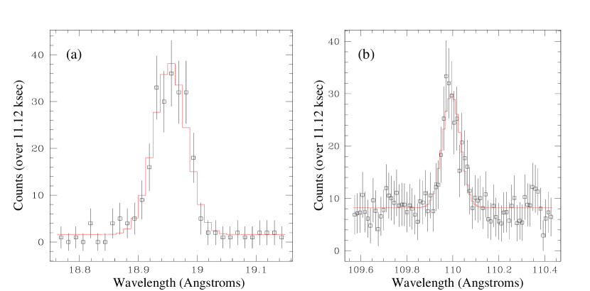
Figure 5: Centroid fits to quarter-phase binned line profiles. The squares are the data and the solid lines are the Gaussian fits to the data obtained using the Sherpa package. (a) The O viii 18.97Å line profile. (b) The profile obtained by summing up the seven strongest lines from the long wavelength region.

Figure 6: Velocity shifts in the line centroids of the O viii 18.97Å profile ($+$ is redshifted while $-$ is blue-shifted). (a) Velocity shifts in the $+1$ and $-1$ orders (dashed and solid lines respectively) are consistent. The squares represent the mean velocity variations of the line profile from both orders and the error bars shown are computed using the errors from the fitting routine in the data analysis package Sherpa. Note that two consecutive phases were observed, the rotation cycle number and phases are calculated using the ephemeris $H\!J\!D=2\,444\,296.575+0.51479E$ (Innis et al. 1988). (b) The phase-folded mean velocity shifts in the line centroids of the Oviii 18.97 Å profile ($+$ is redshifted while $-$ is blue-shifted). The dotted line is the best-fit sine-curve.

The strongest line profiles are converted into velocity-space using the zero-velocity offsets described above. The $+1$ and $-1$ orders are analyzed separately as they have different offsets and systematic distortions. Centroids of the strongest lines in each phase-binned spectrum are also measured using the Gaussian-fitting routine in Sherpa (as done with the zero-velocity calibrations). See Figure 5a for an example of a Gaussian fit to a phase-binned spectral line profile. Centroiding is somewhat compromised in the short wavelength region despite having the highest counts and lowest background due to low spectral resolution. Conversely, at longer wavelengths ($>88$  Å) the spectral resolution improves by a factor of more than 5 but centroiding is difficult due to low counts and a relatively high background.

In this dataset, the strongest line is the O viii 18.97 Å Ly$\alpha$ resonance line (approximately 260 counts total in each phase-binned O viii line profile; see Figure 1). Both the $+1$ and $-1$ orders show remarkably consistent velocity shifts (Figure 6a) despite lines in different orders being subject to different initial offsets and distortions (Chung et al. 2004). The level of agreement between both orders indicates that most systematic effects are averaged out and the modulation shown here is due to the star itself. Figure 6b shows the rotational modulation traced out by the mean of the velocity shifts from both orders. This pattern clearly repeats from one rotation cycle to the next. The largest velocity shift has an amplitude of approximately $40$ $\mbox{km}\,\mbox{s}^{-1}$, a relatively small fraction of AB Dor’s photospheric $v_{e}\,\sin\,i$ value (90 $\mbox{km}\,\mbox{s}^{-1}$). The optimum sine-curve fit to this velocity modulation has a semi-amplitude of $30\pm 10$ $\mbox{km}\,\mbox{s}^{-1}$. We observe no significant variation in the line flux of the phase-binned O viii line profiles. Unfortunately, the lightcurve constructed by integrating the O viii line is too noisy and cannot be used to measure any rotational modulation.

Figure 7: Velocity shifts in the line centroids of the summed line profile (diamonds). The error bars shown here are from Gaussian fitting only, but there are likely to be other sources of error (see text for more details). The rotation cycle and phase have been computed using the ephemeris of Innis et al.’s (1988; see Figure 6b). The sine curve from Figure 6b is also plotted here.

4.1 Centroid shifts at long wavelengths

Since the centroiding accuracy of a line scales with the spectral resolution, the longer wavelength region of the spectrum should in principle be able to confirm the O viii wavelength shifts. Unfortunately, the count rate for individual lines is significantly less than for O viii; however, there are a number of sufficiently strong lines that can be used to produce a composite or summed line profile with a similar signal-to-noise ratio as the Oviii line, following the procedure described by Hoogerwerf, Brickhouse, & Mauche (2004). Taking the quarter-phase binned spectra, we add up the signal from the strongest seven lines at wavelengths greater than 88Å (see Table 1) as follows: the line profiles from both the $+1$ and $-1$ orders are first converted to velocity-space using zero-velocity offsets (computed from the total spectrum), they are then rebinned to the wavelength resolution (32 $\mbox{km}\,\mbox{s}^{-1}$ or 0.012 Å) corresponding to a line at the mean wavelength, 110 Å, and co-added. Figure 5b is an example of a summed line profile. As all the line profiles have slightly different velocity resolutions the summed line profile will not be Gaussian and will be broader than the optimal single line profile.

The centroid position is determined for each quarter-phse summed line profile by fitting Gaussian profiles, as with the O viii line. This method produces centroids close to the flux-weighted mean center, but allows us to make a reasonable error estimate. Figure 7 shows the velocity shifts with these errors in the summed profile as well as the sine-curve fit to the O viii velocity shifts used in Figure 6. While the theoretical accuracy for a Gaussian line with the signal-to-noise ratio of the summed profile is about 5 km s^-1 (see Hoogerwerf, Brickhouse & Mauche 2004), the larger errors ($\sim$16 km s^-1) appear to account for the non-Gaussian nature of the profile, as well as the high background. It should be noted, however, that there are systematic uncertainties in the centroids that may not be accounted for with this method. The “zero velocity” calibration for the individual lines in the total exposure is not as accurate as desired, particularly for the weaker lines, thus introducing additional profile effects. Furthermore, the wavelength distortions associated with the detector read-outs may affect certain measurements. Since each line profile samples two sets of readout taps during a dither cycle, two distinct profiles with different wavelength distortions are always being added. Differences in the amount of time spent on each side can lead to different profile shapes for the same line for different phases. Although we are only interested in relative differences, and the overall wavelength scale appears stable with time, mismatches may add an additional 10 to 15 km s^-1 uncertainty, for the signal-to-noise of the summed profile, to what is derived from the Gaussian fits shown in Figure 7. Improvements to the wavelength scale (Chung et al. 2005) may allow us to exploit the composite line technique with better accuracy in the future. In any case the individual O viii line measurements should be robust.

Table 1: Thermal properties of emission lines.

Wavelength	Ion	Temperature
(Å)		(MK)
18.97	O viii	3.16
88.08	Ne viii	0.631
93.92	Fe xviii	6.31
101.55	Fe xix	7.95
108.37	Fe xix	7.95
117.17	Fe xxii	12.6
128.73	Fe xxi	10.0
132.85	Fe xxiii	12.6

Note. — All lines except O viii were used to generate summed line profiles.

5 Rotational broadening: LETG, HETG & fuse spectra

AB Dor’s photospheric lines are substantially rotationally broadened ($v_{e}\,\sin\,i$$=90$  $\mbox{km}\,\mbox{s}^{-1}$). If the corona is a diffuse shell extended out to several  $\mbox{R}_{*}$, LETG line profiles at long wavelengths should be significantly broader than profiles subject to instrumental and thermal broadening effects alone. While the spectral resolution is limited at short wavelengths, it improves to greater than 2000 above 90 Å and thus enables us to place an upper limit on the extent of the X-ray emitting corona. We measured the width of the strongest emission line profile in the long wavelength region, Fe xviii 93.92 Å. Unfortunately, as Figure 8 shows there is little agreement between the $+1$ and $-1$ order line profiles; when fitting the line profile width we find that the line profile widths are different by a factor of 2. This is a further indication of the large uncertainties in the dispersion scale of the LETG/HRC-S setup at long wavelengths.

Figure 8: The Fe xviii 93.9 Å line profile from the LETG spectra, integrated over 88.1 ksec. The $-1$ and $+1$ orders are plotted left and right respectively. In each plot, the solid line and the filled symbols show the observed data; the dotted line represents the thermally broadened instrumental profile corresponding to a $v_{e}\,\sin\,i$=90 $\mbox{km}\,\mbox{s}^{-1}$ (i.e. the photospheric broadening); the dashed line corresponds to a $v_{e}\,\sin\,i$=250 $\mbox{km}\,\mbox{s}^{-1}$. The $+1$ order profile is significantly narrower than the $-1$ order profile. This is due to large uncertainties in the LETG dispersion calibration at long wavelengths.

As the dispersion scale in the LETG line profiles is unreliable where the spectral resolution is greatest, we measure line profile widths in X-ray and UV datasets of AB Dor obtained in previous years. While the corona of AB Dor may have altered between epochs, these measurements enable us to place a reasonable limit on the extent of the stellar corona. We first look at the Chandra HETG/ACIS-S dataset acquired in 1999 October over 52 ksec (Sanz-Forcada, Maggio & Micela 2003). The spectra are extracted using standard procedures except that pixel randomization is disabled (as with the LETG dataset). In this dataset there are only a handful of strong emission lines that are suitable for this kind of analysis as only the high energy grating (HEG) has sufficient resolution to place a reliable upper limit on the line widths.

In order to evaluate the amount of extra broadening in the line profile after accounting for thermal and instrumental effects, we select the Fe xvii 15.01 Å line profile as it has the least amount of thermal broadening amongst the strongest emission lines in the HEG spectrum. We obtain the instrumental profile for that wavelength from the response matrix file, and convolve this with a Gaussian line profile corresponding to the thermal broadening in the Fe xvii line. This thermally broadened instrumental profile is then convolved with rotation profiles corresponding to different $v_{e}\,\sin\,i$ values, representing different coronal heights. Figure 9 shows the observed line profiles from both the $+1$ and $-1$ orders, with line profiles broadened assuming $v_{e}\,\sin\,i$ values of 90 $\mbox{km}\,\mbox{s}^{-1}$ (dotted line) and 160 $\mbox{km}\,\mbox{s}^{-1}$ (dashed line): corresponding to coronae extending 0.0 $\mbox{R}_{*}$ and 0.75 $\mbox{R}_{*}$ above the stellar surface respectively. As the instrumental and thermal broadening dominate over any small values of rotational broadening, we find that we can only place an upper limit on the extent of the X-ray corona. Our best fit to the spectra implies a corona extending $0.45\pm 0.3$ $\mbox{R}_{*}$ above the stellar surface. Thus we place an upper limit of $\Delta R<0.75$ $\mbox{R}_{*}$ on the coronal extent.

While this upper limit suggests that the bulk of the X-ray emitting corona is contained well within 1 $\mbox{R}_{*}$, its exact extent depends on its geometry, and how the coronal loops are heated. The X-ray emission from coronal loops depends strongly on the orientation of the loop on the stellar disk, the dominant temperature of individual coronal loops and the emissivity of the emission line (Alexander & Katsev 1996, Wood & Raymond 2000). The spectral line fitted here is integrated over a period lasting longer than 1$P_{\mbox{rot}}$ and is thus a global average of all the coronal loops at a range of viewing angles. It should also be noted that some X-ray emission may originate at greater heights but as it would contribute predominantly to the wings of line profiles it would be difficult to detect and measure given the lack of counts. We will present detailed models of AB Dor’s X-ray corona in a future paper based on extrapolations of photospheric magnetic field maps (acquired using a simultaneous dataset) and different heating models.

fuse spectra of the coronal forbidden Fe xviii ($\lambda$974) and Fe xix ($\lambda$1118) lines have a nominal spectral resolution of $\sim$ 20000 and so the line profiles can be resolved. We have re-analyzed the coronal profiles studied by Redfield et al. (2003), and also subjected our more recent and longer fuse observations of AB Dor to analysis (Dupree et al. 2005). Because the lines are weak, a fit to the count spectrum (as opposed to the flux spectrum) is preferred in order to take proper account of the Poisson error distribution and Cash statistics. Moreover we have fit simultaneously the multiple nearby features as well as the coronal iron ions and continuum. Figure 10 shows the Fe xviii transition and the multiple Gaussian fit to the wing of the C iii $\lambda$977 line, and the 2 O i airglow lines. The FWHM of the Fe xviii is 0.59$\pm$0.05 Å for the 2003 data. In addition a similar procedure applied to the 1999 data suggests a Gaussian FWHM of 0.69$\pm$0.1 Å. These fits are overplotted on the data in Figure 10 where the broader line (FWHM =1.0 Å) suggested previously (Redfield et al. 2003) is also shown. Our multiple fitting procedure gives consistent results of a FWHM $\sim$ 0.6 Å for both data sets. The FWHM value of 0.59 Å is to be preferred since the signal is stronger in the longer exposure. The width of the Fe xviii line is very sensitive to the placement of the continuum and the presence of the broadened line wing of C iii. The Fe xix line is more complicated because it is blended with many weak C i lines and possibly an Fe ii line. Nevertheless, the FWHM of the Fe XIX transition, 0.71$\pm$.05 Å, is consistent with the value found for Fe xviii. Our measurements correspond to a coronal height, $\Delta R\approx 0.3\pm 0.2$ $\mbox{R}_{*}$. As before, this value is an average of the corona over all observed phases.

Figure 9: The Fe xvii 15 Å line profile from the HEG spectra of AB Dor taken in 1999, integrated over 52 ksec. The $-1$ and $+1$ orders are plotted left and right respectively. In each plot, the solid line and the filled symbols show the observed data, the dotted line represents the thermally broadened instrumental profile corresponding to a $v_{e}\,\sin\,i$=90  $\mbox{km}\,\mbox{s}^{-1}$ (i.e. the photospheric value); the dashed line corresponds to a $v_{e}\,\sin\,i$=158  $\mbox{km}\,\mbox{s}^{-1}$ ($\Delta R=0.75$  $\mbox{R}_{*}$).

Figure 10: The fuse spectrum from the SiC2A channel of the Fe xviii line region in AB Dor. The lower spectrum was observed in December 2003 (Dupree et al. 2005) with a total exposure time of 108 ks. The upper spectrum (offset at a level of 10 counts) obtained in 1999 (Redfield et al. 2003) had a total exposure time of 24.2 ks. Our multiple Gaussian fit is marked by the broken line where the FWHM of the Fe xviii line is $\sim$ 0.6 Å. A Gaussian curve with a FWHM of 1.0 Å (Redfield et al. 2003) is indicated by the dotted line on the 1999 data.

6 Discussion

The X-ray lightcurve provides strong evidence for rotational modulation in the corona of AB Dor. The strongest peak in the power spectrum of this lightcurve is close to the star’s rotation period of 0.51 day. Sine-curve fitting reveals rotational modulation at the 12% level, consistent with previous estimates made using ROSAT data. The power spectra also have strong peaks at periods corresponding to 0.32 day and 0.18 day. These periods represent shorter term cyclic variations in AB Dor’s corona caused by the presence of three peaks in the lightcurve that are evenly spaced in longitude and stable over a period lasting approximately 1.98 rotation cycles (i.e. the length of our exposure). When studying the X-ray spectra we find that rotational modulation is seen as Doppler shifts in the centroids of phase-binned Oviii line profiles. The centroid shifts trace a roughly sinusoidal pattern that repeats from one cycle to the next with a semi-amplitude of $\pm$30 $\mbox{km}\,\mbox{s}^{-1}$ (Figure 6b). As each line profile is integrated over 0.25$P_{\mbox{rot}}$ the maximum amplitude variation of the centroid of the line profile is likely to be underestimated (by about 11%). If only one compact active region is responsible for this modulation, it would be located at high latitudes, ($\approx 60$^∘). AB Dor’s photospheric $v_{e}\,\sin\,i$ value is 91 $\mbox{km}\,\mbox{s}^{-1}$, so emission from low latitudes would cause Doppler shifts with larger amplitudes and emission from the poles or from a diffuse X-ray emitting corona would not produce any Doppler shifts at all. We can construct a simple model of the emitting corona by combining the diagnostics from the spectra and lightcurves presented in this paper. Our models assume optically thin emission (Ness et al. 2003) and no limb brightening, based on line profiles of the FUSE O VI lines (Redfield et al. 2002).

Figure 11: (a) Chandra/LETG lightcurve folded with AB Dor’s rotation period. Asterisks and diamonds represent consecutive rotation cycles. The horizontal solid line represents the flat, unmodulated emission level while the curves trace the quiescent modulated emission from the star.

As the base level in the lightcurve reveals, approximately 80% of the emission from the star is unchanging. There are two possibilities to explain its lack of modulation: either this component of the X-ray emission originates at the pole of the star and/or this X-ray emission is homogeneously distributed, possibly extending to several stellar radii. However, our analysis of rotational broadening in fuse spectra of AB Dor (albeit from a different epoch) suggests that the bulk of the X-ray emitting corona, where this base level of strong emission would originate, is unlikely to extend more than 0.5 $\mbox{R}_{*}$ above the stellar surface.

The lightcurve also shows three peaks superimposed on the flat, plateau level of X-ray emission. These peaks show evidence of rotational modulation, although some also appear to be intrinsically variable. The shorter-term variations (timescales $\ll 0.05$$P_{\mbox{rot}}$) observed in the lightcurve peaks are likely to be caused by continuous flaring activity. However, we can estimate the quiescent modulation originating in these active regions by tracing the lower envelope of the variability in the lightcurve (Figure 11). Three peaks can be traced (regions A, B and C) in this lightcurve. If we treat each of these peaks as being caused by separate compact (radius $<5$^∘) active regions, we can estimate their locations from the duration of the peaks and dips in the lightcurve. Firstly, as the peaks only last a short time ($<0.5\,\mbox{$P_{\mbox{rot}}$}$) this would suggest that the active regions must be located close to the stellar surface with heights, $H\ll 0.5$ $\mbox{R}_{*}$. Secondly, the compact active regions are separated by over 100^∘ in longitude from each other. As region B is only visible for 0.15$P_{\mbox{rot}}$, it must be located in the partially obscured hemisphere of the star (AB Dor’s inclination angle is 60^∘) between $-55$^∘ and $-60$^∘ latitude with a height, $H\ll 0.5$ $\mbox{R}_{*}$. This region is unlikely to contribute to the centroid shifts in the Oviii line profiles as it takes 0.15$P_{\mbox{rot}}$ to move from the approaching limb to the receding limb. As the phase-binned spectra are integrated over time-bins of 0.25$P_{\mbox{rot}}$, the effective contribution to the centroid shift from this region is zero. Peak C in Figure 11 appears to last 0.22$P_{\mbox{rot}}$ and peak A lasts about 0.45$P_{\mbox{rot}}$. If peaks A and C are caused by separate active regions, they are separated in longitude by 130^∘$\pm 15\mbox{${}^{\circ}$}$. Region C must then also be located in the partially obscured hemisphere at a latitude between $-45$^∘ and $-60$^∘ latitude. Region A can be a small region at equatorial latitudes (radius $<5$^∘, latitude: $-5$^∘ $<\theta<5\mbox{${}^{\circ}$}$) or a larger region at lower latitudes. The most likely explanation for the Oviii line centroid shifts is that they are caused by a net effect due to the relative motions of different, stable emitting regions in both hemispheres. Their exact contribution to the Oviii line centroids would be dependent on the temperatures of the active regions and their relative fluxes.

Table 2: Properties of lightcurve peaks and inferred positions of active regions.

Peak	Phase	Duration	Range of latitudes
		$P_{\mbox{rot}}$
A	0.55	0.45	$-60$∘$\leq\theta\leq 5$∘
B	0.9	0.15	$-60$∘$\leq\theta\leq-55$∘
C	0.2	0.22	$-60$∘$\leq\theta\leq-45$∘
A & C	0.35	0.65	$-60$∘$\leq\theta\leq 40$∘

Note. — Latitudinal positions are estimated assuming compact active regions (radius$\leq 5$^∘).

Alternatively, another scenario that would also fit the observations requires peaks A and C in the lightcurve to arise from one active region. The dip in emission at phase 0.3 could be a shadowing effect caused by cooler material transiting the visible disk at larger heights. Cool prominence-type complexes are commonly detected at heights from 2 $\mbox{R}_{*}$  to 6 $\mbox{R}_{*}$ around AB Dor (e.g. Donati et al. 1999). These clouds have projected areas of between 15% to 20% of the stellar disk as well as absorbing column densities, $N_{H}\approx 10^{20}$ cm^-2 (Collier Cameron et al. 1990; Collier Cameron, Jardine & Donati 200). Evidence for soft X-ray emission being shadowed by cool circumstellar material has been observed on the Sun as well as in stars such as Proxima Centauri and the K dwarf component of the eclipsing binary V471 Tauri (Haisch et al. 1983; Jensen et al. 1986; Walter 2004). The dip that we see near phase 0.3 requires absorbing column densities, $n_{H}\approx 10^{21}$ cm^-2, which are an order of magnitude larger than those estimated by Collier Cameron et al. (1990). Due to incomplete phase coverage of the second rotation phase we are unable to ascertain whether or not this dip is a stable feature in both rotation cycles. The active region in this scenario would be located near the surface, $H<0.3$ $\mbox{R}_{*}$, at latitudes ranging from; $-60$^∘ to $40$^∘, depending on its size. If only one active region causes both peaks C and A as well as the centroid shifts, it should be observable near phase 0.1. Given the large integration times of the phase-binned spectra, a compact active region at 40^∘ latitude might cause both the observed Doppler shifts in the Oviii line profile as well as the lightcurve variability between phases 0.1 and 0.8.

7 Conclusions

To conclude, we construct a simple model of AB Dor’s X-ray emitting corona on the basis of the results discussed in this paper. The observations we seek to fit using this simple model are listed below.

1. Rotationally modulated lightcurve: the lightcurve has a flat level of emission superimposed with three peaks that cause 12% rotational modulation. There is also short-term variability that is probably caused by continuous flaring in active regions.

2. Doppler shifts: The Oviii 18 Å line profile shows a rotationally modulated velocity pattern that repeats in two consecutive rotation cycles. The best-fit sine curve has a semi-amplitude of 30 $\pm 10$ $\mbox{km}\,\mbox{s}^{-1}$.

3. Rotational broadening: Assuming that Doppler broadening is the cause of any excess broadening in the spectral line profiles (once thermal and instrumental effects have been accounted for), we find that the Chandra/HETG Fexvii 15 Å line profiles indicate that the emitting corona does not extend more than 0.75 $\mbox{R}_{*}$ above the stellar surface ($v_{e}\,\sin\,i$$<160$ $\mbox{km}\,\mbox{s}^{-1}$). fuse observations of the coronal forbidden Fexviii and Fexix lines at 974 Å and 1118 Å respectively, suggest an even smaller upper limit of approximately 0.5 $\mbox{R}_{*}$(taking measurement errors into account). These limits assume a global average based on line profiles that have been integrated for a period of more than one rotation period.

Assuming that the rotational modulation in the lightcurves and spectra are caused by the presence of compact active regions, we construct a simple model of AB Dor’s X-ray emitting corona at this epoch. This model has an evenly distributed X-ray emitting corona extending less than 0.5 $\mbox{R}_{*}$ above the stellar surface. There are two to three compact active regions with heights, $H<0.3$ $\mbox{R}_{*}$. Assuming that all three active regions are compact (radii $<5\mbox{${}^{\circ}$}$), two of these regions are located in the partially obscured hemisphere of the (inclined) star at latitudes ranging from $-45$^∘ to $-60$^∘, while the third region may be located closer to the equator.

Alternatively, only one of the compact regions is located in the obscured hemisphere near a latitude, $\theta\sim-55$^∘, and another region is located at higher latitudes, near $40$^∘. In this scenario, the higher latitude region appears to be shadowed by cool absorbing material near phase 0.3. It is likely that the unobscured hemisphere also contains more compact emitting regions, but if they are evenly distributed in longitude they would not cause significant variability in the X-ray lightcurve. However, they would still contribute to the centroid shifts observed in the Oviii line profile.

Spectro-polarimetric ground-based observations of AB Dor were carried out simultaneously with these Chandra observations. We will use Zeeman Doppler imaging techniques to map the surface magnetic field of AB Dor at this epoch, and will extrapolate these surface maps to produce detailed 3-D coronal magnetic field and X-ray emission models (e.g. Hussain et al. 2002, Jardine et al. 2002). In a future paper, we will use this X-ray emission model to predict rotational modulation, rotational broadening in coronal emission lines and compare these models to the X-ray observations presented here.

References

- Ake et al. (2000) Ake, T.B., Dupree, A.K., Young, P.R., Linsky, J.L., Malina, R.F., Griffiths, N.W., Siegmund, O.H.W., Woodgate, B.E. 2000, ApJ, 538, L87
- Alexander & Katsev (1996) Alexander, D. & Katsev, S. 1996, Sol. Phys., 167, 153
- Brandt et al. (2001) Brandt, J.C., Heap, S.R., Walter, F.M., Beaver, E.A., Boggess, A., Carpenter, K.G., Ebbets, D.C., Hutchings, J.B., Jura, M. Leckrone, D.S., Linsky, J.L., Maran, S.P., Savage, B.D., Smith, A.M., Trafton, L.M., Wymann, R.J., Norman, D. & Redfield, S. 2001, AJ, 121, 2173
- Brickhouse et al. (1995) Brickhouse, N.S., Raymond, J.C., Smith, B.W. 1995, ApJS, 97, 551
- Brickhouse & Dupree (1998) Brickhouse, N.S., Dupree, A.K. 1998, ApJ, 502, 918
- Brickhouse, Dupree & Young (2001) Brickhouse, N.S., Dupree, A.K. & Young, P.R. 2001, ApJ, 562, 75
- Chung et al. (2004) Chung, S.M., Drake, J.J., Kashyap, V.L., Ratzlaff, P.W.& Wargelin, B.J. 2004, Proc. SPIE 5165: X-ray and Gamma Instrumentation for Astronomy XIII, eds. K.A. Flanagan, O.H. Siegmund, 518
- Chung et al. (2005) Chung, S.M., Drake, J.J., Kashyap, V.L., Ratzlaff, P.W.& Wargelin, B.J. 2005, Proc. SPIE , in press
- Collier Cameron et al. (1990) Collier Cameron, A., Duncan, D.K., Ehrenfreund, P., Foing, B.H., Kuntz, K.D., Penston, M.V., Robinson, R.D. & Soderblom, D.R. 1990 MNRAS, 247, 415.
- Collier Cameron, Jardine & Donati (2002) Collier Cameron, A., Jardine, M. & Donati, J.-F. 2002, ASP Conf. Proc. 277: Stellar coronae in the Chandra and XMM-Newton Era, eds. F. Favata and J.J. Drake, 397
- Donati et al. (1999) Donati, J.-F., Collier Cameron, A., Hussain, G.A.J. & Semel, M. 1999, MNRAS 392, 437
- Dupree et al. (1993) Dupree, A.K., et al. 1993, ApJ, 418, L41
- Dupree (2001) Dupree, A.K. 2001, Cool Stars, Stellar Systems and the Sun, ASP Conf. Ser. 223 eds. R.J. García Lopez, R. Rebolo, M.R. Zapatero Osorio, 233
- Dupree et al. (2005) Dupree, A.K., et al. 2005, in prep.
- Favata & Schmitt (1999) Favata, F. & Schmitt, J.H.M.M. 1999, A&A, 350, 900
- Favata et al. (2000) Favata, F., Micela, G., Reale, F., Sciortino, S, Schmitt, J.H.M.M. 2000, å, 362, 628
- Güdel et al. (2001) Güdel, M., Audard, M., Magee, H., Franciosini, E., Grosso, N., Cordova, F.A., Pallavicini, R. & Mewe, R. 2001, A&A, 365, L344
- Haisch et al. (1983) Haisch, B.M., Linsky, J.L., Bornmann, P.L., Stencel, R.E., Antiochos, S.K., Golub, L. & Vaiana, G.S. 1983, ApJ, 267, 280
- Hoogerwerf, Brickhouse & Mauche (2004) Hoogerwerf, R., Brickhouse, N.S. & Mauche, C.W. 2004, ApJ, 610, 411
- Hussain (2002) Hussain, G.A.J 2002, AN, 323, 349
- Hussain et al. (2002) Hussain, G.A.J, van Ballegooijen, A., Jardine, M. & Collier Cameron, A. 2002, ApJ, 575, 1078
- Innis et al. (1988) Innis, J.L., Thompson, K., Coates, D.W., Evans, T.L. 1988 MNRAS, 235, 1411
- Jardine et al. (2002) Jardine, M., Wood, K., Collier Cameron, A., Donati, J.-F., Mackay, D.H., 2002, MNRAS, 336, 1364
- Jensen et al. (1986) Jensen, K.A., Swank, J.H., Petre, R., Guinan, E.F., Sion, E.M. & Shipman, H.L. 1986, ApJ, 309, L27
- Kürster et al. (1997) Kürster, M., Schmitt, J.H.M.M., Cutispoto, G. & Dennerl, K. 1997, A&A, 320, 831
- Lammer et al. (2003) Lammer, H., Selsis, F., Ribas, I., Guinan, E.F., Bauer, S.J. & Weiss, W.W. 2003, ApJ, 598, L121
- Maggio et al. (2000) Maggio, A., Pallavicini, R., Reale, F. & Tagliaferri, G. 2000, A&A, 356, 627
- Ness et al. (2003) Ness, J.-U., Schmitt, J.H.M.M., Audard, M., Güdel, M., Mewe, R. 2003, A&A, 407, 347
- Orlando et al. (2000) Orlando, S., Peres, G. & Reale, F. 2000, ApJ, 528, 524
- Redfield et al. (2002) Redfield, S., Linsky, J.L., Ake,T.B., Ayres, T.R., Dupree, A.K., Robinson, R.D., Wood, B.E. & Young, P.R. 2002, ApJ, 581, 626
- Refield et al. (2003) Redfield, S., Ayres, T.A., Linsky, J.L., Ake, T.B., Dupree, A.K., Robinson, R.D. & Young, P.R. 2003, ApJ, 585, 993
- Sanz-Forcada, Brickhouse & Dupree (2002) Sanz-Forcada, J., Brickhouse, N.S. & Dupree, A.K. 2002, ApJ, 570, 799
- Sanz-Forcada, Maggio & Micela (2003) Sanz-Forcada, J., Maggio, A., Micela, G. 2003, A&A, 408, 1087
- Schmitt (1998) Schmitt, J.H.M.M., 1998, ASP Conf. Ser. 154: Cool Stars, Stellar Systems and the Sun, eds. Donahue, R.A. and Bookbinder, J.A., 463,
- Schmitt & Favata (1999) Schmitt, J.H.M.M. & Favata, F. 1999, Nature, 401, 44
- (36) Solanki, S.K., Motamen, S. & Keppens, R. 1997, A&A, 325, 1039
- Stelzer et al. (2002) Stelzer, B., Burwitz, V., Audard, M., Güdel, M., Ness, J.-U., Grosso, N., Neuhäuser, R., Schmitt, J.H.M.M., Predehl, P. & Aschbach, B. 2002, A&A, 392, 585
- Unruh, Collier Cameron & Cutispoto (1995) Unruh, Y.C., Collier Cameron, A. & Cutispoto, G. 1995, MNRAS277, 1145
- Vilhu & Linsky (1987) Vilhu, O. & Linsky, J.L. 1987, PASP, 99, 1071
- (40) Walter, F.M. 2004, AN, 325, 241
- Wood & Raymond (2000) Wood, K. & Raymond, J. 2000, ApJ, 540, 563