The Parkes H i Survey of the Magellanic System

We present the first fully and uniformly sampled, spatially complete H i survey of the entire Magellanic System with high velocity resolution ($\Delta v$ = 1.0 km s^-1), performed with the Parkes Telescope. Approximately 24 percent of the southern sky was covered by this survey on a $\approx$ 5′ grid with an angular resolution of HPBW = 14$\aas@@fstack{\prime}$1. A fully automated data-reduction scheme was developed for this survey to handle the large number of H i spectra ($1.5\times 10^{6}$). The individual Hanning smoothed and polarization averaged spectra have an rms brightness temperature noise of $\sigma$ = 0.12 K. The final data-cubes have an rms noise of $\sigma_{\rm rms}\approx$ 0.05 K and an effective angular resolution of $\approx$16′. In this paper we describe the survey parameters, the data-reduction and the general distribution of the H i gas.
The Large Magellanic Cloud (LMC) and the Small Magellanic Cloud (SMC) are associated with huge gaseous features – the Magellanic Bridge, the Interface Region, the Magellanic Stream, and the Leading Arm – with a total H i mass of $M$(H i) = 4.87$\cdot$10⁸ M${}_{\odot}\left[d/55\leavevmode\nobreak\ {\rm kpc}\right]^{2}$, if all H i gas is at the same distance of 55 kpc. Approximately two thirds of this H i gas is located close to the Magellanic Clouds (Magellanic Bridge and Interface Region), and 25% of the H i gas is associated with the Magellanic Stream. The Leading Arm has a four times lower H i mass than the Magellanic Stream, corresponding to 6% of the total H i mass of the gaseous features.
We have analyzed the velocity field of the Magellanic Clouds and their neighborhood introducing a LMC-standard-of-rest frame. The H i in the Magellanic Bridge shows low velocities relative to the Magellanic Clouds suggesting an almost parallel motion, while the gas in the Interface Region has significantly higher relative velocities indicating that this gas is leaving the Magellanic Bridge building up a new section of the Magellanic Stream. The Leading Arm is connected to the Magellanic Bridge close to an extended arm of the LMC. The clouds in the Magellanic Stream and the Leading Arm show significant differences, both in the column density distribution and in the shapes of the line profiles. The H i gas in the Magellanic Stream is more smoothly distributed than the gas in the Leading Arm. These morphological differences can be explained if the Leading Arm is at considerably lower z-heights and embedded in a higher pressure ambient medium.

1 Introduction

The Magellanic Clouds are irregular dwarf galaxies orbiting the Milky Way. The distances for the Large Magellanic Cloud (LMC) and the Small Magellanic Cloud (SMC) are 50 and 60 kpc, respectively (see Walker walker (1999) and references therein). The Magellanic Clouds possess a huge amount of gas – in contrast to the Sagittarius dwarf spheroidal galaxy (Sgr dSph, Ibata et al. ibata (1994)), which does not currently contain neutral hydrogen (Koribalski et al. koribalski (1994); Burton & Lockman burton (1999); Putman et al. 2004a ).

The Magellanic Clouds were first detected in H i by Kerr et al. (kerr (1954)). The detailed distribution of H i in the LMC was first described by Kerr & de Vaucouleurs (kerr2 (1955)) and McGee (mcgee (1964)). Hindman et al. (hindman (1961)) discovered that the two galaxies are embedded in a common envelope of H i gas. The gas connecting the Magellanic Clouds is called the Magellanic Bridge. The H i distribution and dynamics in the LMC were reexamined by Rohlfs et al. (rohlfs (1984)), by Luks & Rohlfs (luks (1992)), and more recently by Staveley-Smith et al. (stavele2 (2003)). Single-dish observations of the H i gas, using the 64-m Parkes telescope, have a spatial resolution of about 225 pc $\left[d/55\,{\rm kpc}\right]$. These data have sufficient angular resolution to study the large-scale distribution of the H i gas in the Magellanic System. H i studies at high angular resolution were performed by Kim et al. (kim (1998), kim2 (2003)) for the LMC and by Stanimirovic et al. (stanimirovic (1999), stanimirovic3 (2004)) for the SMC, using the Australia Telescope Compact Array (ATCA). These observations revealed a fractal structure of the ISM in these galaxies and detected structure down to the resolution limit.

Dieter (dieter (1965)) surveyed the Galactic poles with the Harvard 60-ft antenna and noted several detections with high radial velocities near the southern Galactic Pole, which have no counterparts towards the northern pole. This was the first detection in H i 21-cm line emission of what we today call the “Magellanic Stream”, but she did not identify it as a coherent structure. Further observations of the northern part of the Magellanic Stream, called the “south pole complex” at this time, were performed by Kuilenburg (kuilenburg (1972)) and Wannier & Wrixon (wannier (1972)). Mathewson et al. (mathewson (1974)) observed the southern part of the Magellanic Stream using the 18-m Parkes telescope. They discovered the connection between the “south pole complex” and the Magellanic Clouds and called it the “Magellanic Stream”. Later on, several parts of the Magellanic Stream were observed with higher resolution and sensitivity (e.g. Haynes haynes (1979); Cohen cohen (1982); Morras morras (1983),morras2 (1985); Wayte wayte (1989); Stanimirovic et al. stanimirovic2 (2002); Putman et al. 2003a ).

Wannier et al. (wannier2 (1972)) discovered high-positive-velocity clouds close to the Galactic Plane. Several clouds in this region were subsequently observed with higher resolution and sensitivity (e.g. Mathewson et al. mathewson (1974); Giovanelli & Haynes giovanelli (1976); Mathewson et al. mathewson3 (1979); Morras morrasa (1982); Morras & Bajaja morrasbajaja (1983); Bajaja et al. bajaja (1989); Cavarischia & Morras cavarischia (1989); Putman et al. putman (1998); Wakker et al. wakker2 (2002)).

Recently, two large-scale surveys have been completed, covering the southern sky. The first is the Argentinian H i Southern Sky Survey (HISSS), presented by Arnal et al. (arnal (2000)) and Bajaja et al. (bajaja04 (2004)). HISSS is the counterpart to the Leiden/Dwingeloo survey of Galactic neutral atomic hydrogen (Hartmann & Burton hartmann (1997)) and offers an angular resolution of 30′ with grid spacings of 30′. The velocity resolution is $\Delta v$ = 1.3 km s^-1 and the rms noise is $\sigma_{\rm rms}\approx$ 0.07 K. A combined all-sky H i survey is presented by Kalberla et al. (kalberla04 (2004)). The second survey is the H i Parkes All Sky Survey (HIPASS, Barnes et al. barnes (2001)), that was performed using the multi-beam facility of the Parkes telescope (Staveley-Smith et al. stavele1 (1996)). It offers a velocity resolution of $\Delta v$ = 16 km s^-1 and an rms noise of $\sigma_{\rm rms}\approx$ 0.01 K. The observing mode of the HIPASS is in-scan beam-switching. This mode filters out all large-scale structure of the Milky Way or the Magellanic System. Recently, routines were developed to recover the majority of the extended structure in the features of the Magellanic System (Putman et al. 2003a ).

This paper presents the Parkes narrow-band H i survey of the Magellanic System, designed not only to study the system at high velocity resolution, but to retain sensitivity to all spatial scales. Section 2 describes the survey parameters, the observations and the data-reduction in detail. Section 3 presents the H i in the Magellanic Clouds and their immediate vicinity. Section 4 describes the Interface Region and isolated clouds in the vicinity of the Magellanic Clouds. Sections 5 and 6 present the H i in the Magellanic Stream and the Leading Arm, respectively. Section 7 gives a summary and conclusions.

Figure 1: Two example spectra from one scan. a) original raw spectra. The individual observed bandpasses comprise not only different amounts of astronomical line emission, but also a varying amount of continuum emission due to astronomical sources, radiation from the ground etc. b) the same spectra after scaling with T_sys. The scaled spectra are almost identical, indicating that the shape of the bandpass is very stable with time.

2 Observations and Data-Reduction

2.1 Observations

The Parkes telescope has a parabolic reflector with a diameter of 64 m that can be operated above 30° elevation. At 21 cm, a multi-beam facility with 13 beams is available, offering a half power beam width (HPBW) of 14$\aas@@fstack{\prime}$1. All 13 beams are, however, usable only in wide-band mode, operating with a bandwidth of 64 MHz with 1024 channels per polarization. This mode is well suited for extra-galactic surveys like HIPASS. Observing modes with a higher velocity resolution (the narrow-band modes) utilize the central seven beams in a hexagonal configuration. These beams are much more symmetric than the outer beams, 8 – 13, which suffer from coma distortion. For this survey, we used the narrow-band mode with 8 MHz bandwidth, offering 2048 autocorrelator channels for each beam and polarization. The bandwidth of 8 MHz corresponds to a velocity coverage of 1690 km s^-1. The channel spacing of 3.91 kHz corresponds to a velocity spacing of 0.825 km s^-1, while the effective velocity resolution is 1.0 km s^-1. Our survey has therefore a 16 times higher velocity resolution than HIPASS.

The H i observations of the Magellanic System were performed within 11 days from February 17th to 21st and from November 2nd to 8th 1999. The data were taken using the so-called in-band frequency-switching mode. The central frequencies of the two spectra (“signal-” and “reference-spectrum”) are chosen in a way that the “reference-spectrum” also contains the spectral line. A frequency offset of 3.5 MHz between both signals was chosen for our survey. The advantage of this method is that the telescope is on-source all the time.

The multi-beam receiver can be rotated by feed-angles between –60 and 60 degrees. The feed-angle was set to 19$\aas@@fstack{\circ}$1 relative to the direction of the scan to provide uniform sampling. The H i data were observed in on-the-fly mode with a telescope scanning speed of 1′ per second. The integration time per spectrum was set to 5 seconds for both frequencies. The beam moves 5′ on the sky during the integration, leading to a slightly elongated beam in direction of the scan. The scans were aligned to Magellanic coordinates, as both the southern poles of Equatorial and Galactic coordinates fall into the region of interest. The scans were taken in direction of Magellanic latitude at constant longitude. The scans had a length of 15° for most observed fields. The offset between two adjacent scans (in Magellanic longitude) was set to 66$\aas@@fstack{\prime}$7. A feed-angle of 19$\aas@@fstack{\circ}$1 yields beams moving along equidistant lines with a separation of 9$\aas@@fstack{\prime}$358. Each field was observed a second time with an offset of 33$\aas@@fstack{\prime}$6. The combined data have grid-spacings of 5′ in the direction of the scan (Magellanic Latitude) and 4$\aas@@fstack{\prime}$679 perpendicular to the scan direction (Magellanic Longitude). The comparison with the HPBW of 14$\aas@@fstack{\prime}$1 demonstrates that the data have a higher sampling than required by the Nyquist-sampling theorem.

We utilized early HIPASS maps from Putman et al. (2003a ) to define the regions of interest with emission from the Magellanic Clouds and their gaseous arms. In total, 745 598 individual pointings, covering approximately 24 percent of the southern sky, were observed.

2.2 Data-Reduction

A total number of 1 491 196 source spectra were observed for the Parkes narrow-band survey of the Magellanic System. Due to the large number of spectra an automated reduction pipeline was a necessity.

2.2.1 Bandpass Calibration

We used the standard method to perform the bandpass calibration:

$$T_{\rm A} = T_{\rm sys}\leavevmode\nobreak\ \frac{T_{\rm sig}-T_{\rm ref}}{T_{\rm ref}}.$$ (1)

For in-band frequency switching, both $T_{\rm sig}$ and $T_{\rm ref}$ contain the spectral lines shifted by 3.5 MHz. In the course of the data-reduction it became clear that the baselines are highly non-linear – a polynomial of 8th order is needed to fit most baselines. It is extremely difficult to separate baseline wiggles from faint emission lines. Even a large amount of work failed to produce sufficiently flat baselines with an automated pipeline. Accordingly, a different approach was taken which involved searching for individual reference positions for each spectral channel.

The individual observed bandpasses not only have different amounts of astronomical line emission along the scan, but also a varying amount of continuum emission. Figure 1a shows two randomly chosen raw-spectra of a scan containing a different amount of continuum emission. Figure 1b shows the same spectra after division by T_sys. The scaled spectra are almost identical (expect for varying line emission). The spectra of a scan of the same beam, polarization and central frequency have almost the same shape, while the shape of the bandpass varies strongly for different beams, polarizations and central frequencies.

The stability of the shape of the bandpass can be used to perform the bandpass calibration. Scans were taken in a manner such that each scan has, at a given velocity, an appreciable length free of Magellanic emission. A reference spectrum is compiled by searching for emission free regions for each velocity. This is done by dividing the scan into smaller parts (e.g. ten subscans). For each subscan, beam, polarization, and frequency a median of the values for each individual spectral channel is calculated. The minimum of these medians for a given channel is taken for each beam, polarization, and frequency. The method is similar to the MINMED5 method described by Putman et al. (2003a ).

This method produces 28 bandpasses, one for each beam, polarization and center frequency. These bandpasses are free from emission from the Magellanic System, but they still contain emission from the extended gas of the Milky Way and “extended” radio frequency interference (RFI) that is apparent in all spectra of a scan. Some more steps are necessary to recover also the extended emission, e.g. the H i from the local gas of the Milky Way. The remaining spectral features have in general line widths of a few channels in the case of RFI and 10 to 25 channels in the case of Galactic emission, while the baseline varies on much larger numbers of channels with lower amplitude. The bandpass for each beam, polarization and center frequency is now searched for lines by looking for a steep rise of more than 1 K over 8 channels. These identified regions are enlarged by $\pm$50 channels to guarantee that the whole line including possible extended line wings are included. An initial 6th-order polynomial is subtracted from the bandpasses. Every channel that was classified as being free of emission is now re-examined. If the intensity of the fitted spectrum at a channel is higher than 0.65 K the channel is classified as having line emission. The newly identified line windows are extended as described above and applied to the original bandpasses. The procedure is repeated with a threshold of 0.3 K.

A polynomial of 6th order is fitted to the bandpass using the final spectral line mask. The values within the line windows are replaced by the polynomial, while the other channels remain unchanged. This routine yields 28 reference bandpasses that are free from line emission and strong RFI. These final bandpasses are now applied to all spectra of the scan using Eq. 1.

2.2.2 Baseline Correction and RFI Subtraction

The bandpass calibrated spectra have in general quite flat baselines. For most spectra ($\approx$ 97%) a linear baseline subtraction is sufficient. The remaining spectra have baselines where a polynomial of third order is needed. To compute the final baseline, a spectral mask is again required. This mask is calculated as described above.

The spectra available at this point are bandpass calibrated and have flat baselines, but are still contaminated by RFI. In the case of the Parkes narrow-band survey, only sinc-shaped RFI is present. After Hanning smoothing, spikes with a width of one or two channels are present. These interferences appear at the same channels over the whole scan (no Doppler tracking has been applied so far). The identification process averages and Hanning smoothes all spectra for each beam, polarization and center frequency. Every spectral feature in the averaged spectra with a width of one or two channels with an intensity larger than 0.25 K is recognized as RFI. The values at these channels are substituted by a linear interpolation of the neighboring channels for all individual spectra.

In the very last step the rest-frame of the velocity is converted from topocentric to the local-standard-of-rest (LSR) frame.

2.2.3 Gain Calibration

The H i data were calibrated to brightness temperature scale using the standard calibration sources S8 and S9 (Williams williams (1973)). We used the well defined flux of S8 at 14′ resolution from Kalberla et al. (kalberla (1982)) as primary calibrator and derived a brightness temperature of $T_{\rm B}$ = 83 K for S9. The calibration source S9 served as secondary calibrator to monitor the calibration. The parameters of the calibration sources are summarized in Table 1.

Table 1: Parameters of the calibration sources S8 and S9.

	l	b	RA (J2000)	DEC (J2000)	Tmax
S8	207$\aas@@fstack{\circ}$00	–15$\aas@@fstack{\circ}$00	5h47m21.3s	–1∘40’18.4”	76 K
S9	356$\aas@@fstack{\circ}$00	–4$\aas@@fstack{\circ}$00	17h52m05.4s	–34∘25’15.4”	83 K

The calibrators were observed by each of the seven beams independently and in turn. The calibration source S8 was observed 4 times and S9 7 times. The standard deviations of the calibration factors for each individual beam, polarization and center frequency are lower than one percent, demonstrating that the calibration factors are very stable over a period of a couple of days.

In addition to the pointed observations, S9 was observed five times using the on-the-fly mode to make sure that the results derived from pointed observations do not differ from the on-the-fly data. The standard deviation of the intensity at the position of S9 is 0.53 percent around the nominal value of 83 K.

2.3 Stray-Radiation

Table 2: Observational parameters of the H i survey.

Antenna diameter	64 m
HPBW	14$\aas@@fstack{\prime}$1
Observing mode	on-the-fly mapping
Sky coverage	$\approx$24%
Number of spectra	1 491 196
Grid in Magellanic Coord.	4$\aas@@fstack{\prime}$679, 5′
Integration time per spectrum	5 sec.
Total bandwidth	8 MHz
Usable bandwidth	4.5 MHz
Usable velocity coverage	950 km s-1
Original velocity resolution	1.0 km s-1
Channel separation	0.825 km s-1
Velocity resolution after Hanning smooth	1.65 km s-1
RMS noise after Hanning smooth	0.12 K
Final data cubes:
Angular resolution	16′
RMS noise	0.05 K

The observed antenna temperature, $T_{\rm A}$, can be transformed to brightness temperature, $T_{\rm B}$, using the equation from Kalberla et al. (kalberla2 (1980)):

$$T_{\rm B}\left(\vartheta,\phi,v\right) = \frac{1}{\eta_{\rm MB}}T_{\rm A}\left(\vartheta,\phi,v\right)$$

$$-\frac{1}{\eta_{\rm MB}}\int_{\rm SL}P\left(\vartheta-\vartheta^{\prime},\phi-\phi^{\prime}\right)T_{\rm B}\left(\vartheta^{\prime},\phi^{\prime},v\right){\rm d}\Omega^{\prime},$$

where $\eta_{\rm MB}$ is the mainbeam efficiency and $P$ is the antenna diagram. The second line gives the contribution from the side-lobes (SL) also known as stray-radiation. The entire sky is covered by H i emission at low velocities ($v\approx 0$ km s^-1). Kalberla et al. (kalberla2 (1980)) demonstrated that the total amount of stray-radiation for Galactic emission is typically about 15% of the observed profile area, but it can increase to 50% or more at high Galactic latitudes.

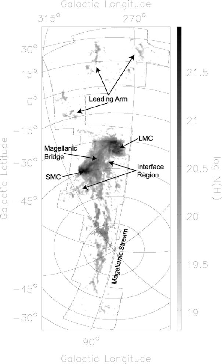
Figure 2: H i column density distribution of the entire Magellanic System. H i emission associated with the Milky Way (see Fig. 3) was omitted. Note that the radial velocities of the Magellanic Stream are close to Galactic velocities near ($l$,$b$) = (315°, –80°). The emission of this gas was recovered as described in Sect. 5.3. The grey-scale is logarithmic and represents column densities between $N$(H i) = 6$\cdot$10¹⁸ cm^-2 (light grey) and $N$(H i) = 9$\cdot$10²¹ cm^-2 (black). The black contours indicate the borders of the survey. Zero longitude is to the left.

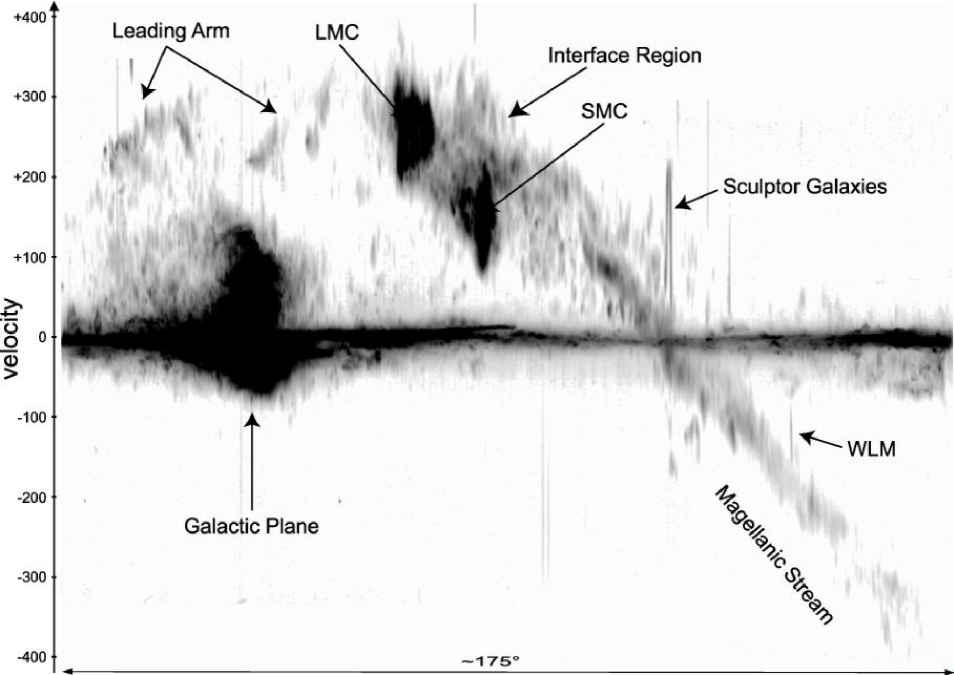
Figure 3: The figure shows a position/velocity peak intensity map of the data-cube shown in Fig. 2: radial velocity ($v_{\rm LSR}$) is plotted as a function of position (corresponding to the y-axis of the data-cube presented in Fig. 2). The grey-scale indicates the peak intensity (along the x-axis of the data-cube presented in Fig. 2). White corresponds to $T_{\rm B}=0$ K, black corresponds to $T_{\rm B}>15$ K. The figure shows the Magellanic Clouds and the associated gaseous features, the local gas of the Milky Way (near $V_{\rm LSR}$ = 0 km s^-1), and some galaxies (see Fig. 8).

The Parkes narrow-band H i survey of the Magellanic System has not been corrected for stray-radiation. The Galactic emission is certainly affected by stray-radiation from the near and far side-lobes of the antenna pattern. While the general distribution can be studied, no quantitative analysis of the Milky Way H i emission is possible using our data.

However, the neutral hydrogen associated with the Magellanic System is clearly separated from Galactic emission, except for a small region close to the southern Galactic Pole. At high velocities only a very small fraction of the sky is covered by H i emission at each individual velocity, leading to a negligible integral over the side-lobe region (see Eq. 2.3). A stray-radiation correction for the H i emission of the gaseous features of the Magellanic System is therefore not necessary.

2.4 Data-cubes and final sensitivity

The H i data of the Parkes narrow-band survey of the Magellanic System have grid-spacings of 5′ in the direction of the scan (Magellanic Latitude) and 4$\aas@@fstack{\prime}$679 perpendicular to the scan direction (Magellanic Longitude). At each position, two independent spectra (the two polarizations) are available, leading to an 1-$\sigma$ rms brightness temperature noise of $\sigma_{\rm rms}\approx$ 0.12 K in the averaged and Hanning smoothed spectra.

The aim of this paper is to present the large-scale distribution and morphology of the H i gas in the Magellanic System at high sensitivity. We choose Galactic coordinates for all maps in this paper to simplify a comparison with features in the Milky Way. A higher signal-to-noise ratio can be achieved by modest spacial smoothing. The data-cubes presented in this paper are gridded using the GRIDZILLA tool that is part of AIPS++. The true angle grid-spacings in the data-cubes are set to 4′. For each grid point, neighboring spectra within a diameter of 8′ are taken into account. These spectra are weighted by a Gaussian with FWHM of 8′. This spacial smoothing increases the effective beam size to $\approx$16′, but improves the rms noise to about $\sigma_{\rm rms}\approx$ 0.05 K at a velocity resolution of $\Delta v$ = 1.65 km s^-1.

A 1-$\sigma$ signal of $T_{\rm B}$ = 0.05 K corresponds to a column density of $N$(H i) = 1.5$\cdot$10¹⁷ cm^-2 per spectral channel ($\Delta v$ = 1.65 km s^-1). Typical H i lines from clouds consisting of warm neutral gas, however, show line widths of typically $\Delta v_{\rm FWHM}\approx$ 25 km s^-1. A Gaussian line with a peak intensity at the 5-$\sigma$ level and a line width of $\Delta v_{\rm FWHM}\approx$ 25 km s^-1 corresponds to a column density of approximately $N$(H i) = 1.2$\cdot$10¹⁹ cm^-2. These values give an idea of what is detectable in the maps we show in this paper, while even weaker lines can be detected applying further smoothing.

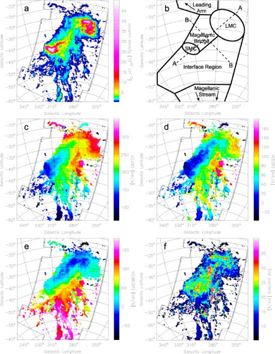
Figure 4: a) The H i column density map of the Magellanic Clouds and their environment. The black contours indicate the borders of the survey. The LMC and the SMC are connected by the Magellanic Bridge. The Interface Region connects the Magellanic Clouds and the Magellanic Bridge with the Magellanic Stream. b) A schematic view of the LMC, the SMC and the neighboring H i gas. The arrows indicate that the Magellanic Stream and the Leading Arm continue outside the borders of this map. The dashed lines marked with A and B indicate the position of the slices shown in Figs. 5 and 7, respectively. c) The velocity field in the local-standard-of-rest frame. d) The velocity field in the Galactic-standard-of-rest frame. e) The velocity field in the LMC-standard-of-rest frame (see Sect. 3.2). f) The 2nd moment map.

The HISSS survey (Arnal et al. arnal (2000)) has a typical rms of the order $\sigma_{\rm rms}\approx$ 0.07 K at a velocity resolution of $\Delta v$ = 1.3 km s^-1. HISSS has an angular resolution of 30′ and grid spacings of 30′, i.e. it is not fully sampled. Our survey has a higher angular resolution and full sampling. We reach an rms noise of the order $\sigma_{\rm rms}\approx$ 0.017 K when smoothing to the angular resolution of HISSS.

HIPASS HVC maps have a typical rms of the order $\sigma_{\rm rms}\approx$ 0.008 K at a velocity resolution of $\Delta v$ = 26.0 km s^-1 (Putman et al. 2003a ). Our survey has an rms noise of $\sigma_{\rm rms}\approx$ 0.012 K when smoothing to the same velocity resolution, demonstrating that HIPASS has a slightly higher sensitivity than our survey. The higher velocity resolution and the reduction being optimized for the recovery of extended emission makes our survey ideal for a detailed study of the Magellanic System.

Figure 2 shows an H i column density map of the Magellanic Clouds (Sect. 3), the Magellanic Bridge (Sect. 3), the Interface Region (Sect. 4), the Magellanic Stream (Sect. 5), and the Leading Arm (Sect. 6). The map covers the entire area covered by our survey; the contours represent the borders of our survey. The H i emission of the Milky Way was omitted. Figure 3 shows a position/velocity peak intensity map of the data-cube shown in Fig. 2, where the position corresponds to the y-axis of that data-cube. The grey-scale indicates the peak intensity along the x-axis of that data-cube. The individual gaseous features shown in Figs. 2 and 3 are discussed in the following sections.

3 H i in the Magellanic Clouds and the Magellanic Bridge

3.1 The column density distribution

The Large and the Small Magellanic Cloud are H i rich dwarf irregular galaxies located on the southern sky at (l,b) = (280$\aas@@fstack{\circ}$5, –32$\aas@@fstack{\circ}$9) and (302$\aas@@fstack{\circ}$8, –44$\aas@@fstack{\circ}$3), respectively (see Westerlund westerlund (1997) for a review). Figure 4a shows the H i column density distribution of the Magellanic Clouds and their environment. Both galaxies are embedded in a common H i envelope covering tens of degrees on the sky. The angular extent of the Magellanic Clouds is therefore not well defined in H i. The gas connecting the Magellanic Clouds is called the Magellanic Bridge (Hindman et al. hindman (1961)). Figure 4b shows a schematic overview of this region and the location of the individual gaseous features.

The peak column densities of the LMC and the SMC are $N$(H i) = 5.5$\cdot$10²¹cm^-2 and $N$(H i) = 1.01$\cdot$10²²cm^-2, respectively. H i column densities above $N$(H i) = 1$\cdot$10²¹cm^-2 are common in both galaxies. Stanimirovic et al. (stanimirovic (1999)) studied the H i gas of the SMC in great detail. They analyzed H i absorption measurements and concluded that regions with H i column densities greater than $N$(H i) = 2.5$\cdot$10²¹cm^-2 are affected by self-absorption. The peak column densities stated above are therefore only lower limits.

The H i gas outside the Magellanic Clouds has much lower column densities. Typical column densities in the Magellanic Bridge are $N$(H i) $\approx 5\cdot$10²⁰cm^-2. This emission can be considered as optically thin (Stanimirovic et al. stanimirovic (1999)).

The H i gas of the LMC has recently been studied in detail by Kim et al. (kim2 (2003)) and by Staveley-Smith et al. (stavele2 (2003)). The SMC was studied recently by Stanimirovic et al. (stanimirovic3 (2004)). The SMC shows an irregular morphology with a high column density tail pointing towards the LMC. A recent study of the H i in the tail was performed by Muller et al. (2003a ). This tail hosts a stellar component and is also known as Shapleys Wing (Shapley shapley (1940)). The Wing hosts a number of young stars (e.g. Sanduleak sanduleak (1969)) and molecular clouds (Muller et al. 2003b ).

3.2 The Velocity Field

The Parkes multi-beam survey of the Magellanic System provides spectra in the local-standard-of-rest frame. The velocity field of the H i data is analyzed using the first moment of the spectra, i.e. the intensity weighted mean velocity, $\overline{v_{\rm LSR}}$, that is calculated by

$$\overline{v_{\rm LSR}}=\frac{\Sigma(T_{{\rm B},i}\cdot v_{i})}{\Sigma T_{{\rm B},i}},$$ (3)

where $T_{{\rm B},i}$ and $v_{i}$ indicate the brightness temperature and the radial velocity at channel $i$, respectively.

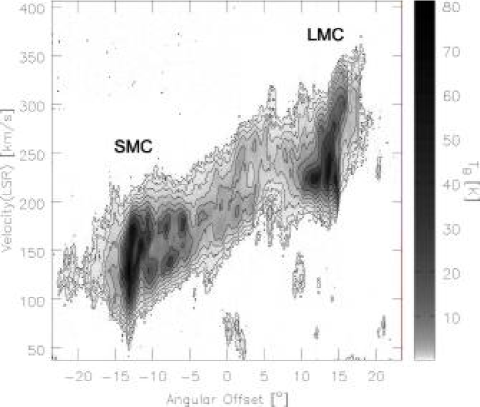
Figure 5: A position/velocity slice through the data-cube shown in Fig. 4 from ($l$,$b$) = (314$\aas@@fstack{\circ}$0, -48$\aas@@fstack{\circ}$0) to (275$\aas@@fstack{\circ}$0, -25$\aas@@fstack{\circ}$5). The position of this slice is marked in Fig. 4b by the dashed line A. Contour lines start at $T_{\rm B}$ = 0.15 K (3$\sigma$) and increase by factors of two, i.e. $T_{\rm B}$ = 0.3, 0.6, 1.2, 2.4, 4.8, 9.6, 19.2, 38.4 K.

Figure 4c shows the observed velocity field of the Magellanic Clouds and their neighborhood. The observed velocities cover the velocity interval from $v_{\rm LSR}=$ 120 km s^-1 in the SMC to $v_{\rm LSR}=$ 300 km s^-1 in the LMC. Figure 5 shows an exemplary slice through the data-cube presented in Fig. 4, demonstrating that the H i gas smoothly connects both Magellanic Clouds in the position/velocity space. The systemic velocities of the Magellanic Clouds differ by $\Delta v_{\rm LSR}$ = 125 km s^-1.

The local-standard-of-rest frame is not the best suited reference system as the Magellanic Clouds form a large system far from the solar neighborhood. The varying angle between the line-of-sight and the solar velocity vector introduces an artificial velocity gradient that is not related to the Magellanic Clouds. This effect can be overcome by transforming the radial velocities to the Galactic-standard-of-rest frame using

$$v_{\rm GSR}=v_{\rm LSR}+220\leavevmode\nobreak\ {\rm sin}\leavevmode\nobreak\ l\leavevmode\nobreak\ {\rm cos}\leavevmode\nobreak\ b,$$ (4)

where $l$ and $b$ are Galactic longitude and latitude, respectively. Velocities are measured in km s^-1 and 220 km s^-1 corresponds to the velocity of the solar circular rotation around the Milky Way. Figure 4d shows the same region as Fig. 4c, but the velocities are transformed to the Galactic-standard-of-rest frame. The velocity difference between the Magellanic Clouds decreases from $\Delta v_{\rm LSR}$ = 125 km s^-1 to $\Delta v_{\rm GSR}$ = 67 km s^-1. The highest radial velocities in the GSR frame are found in the Interface Region and the Leading Arm, while the gas in the Magellanic Bridge shows low velocities indicating either low total velocities or velocity vectors that are almost perpendicular to the lines-of-sight. Unfortunately, the velocity vectors of H i clouds are not directly observable. The velocity vectors of the Magellanic Clouds, however, have been estimated from stellar data recently (Kroupa & Bastian kroupa (1997); van der Marel marel (2002)). The results from Kroupa & Bastian (kroupa (1997)) demonstrate that the Magellanic Clouds have almost parallel velocity vectors, but very different radial velocities due to projection effects. We would therefore observe a velocity gradient across the Magellanic Bridge even if all clouds had the same velocity vector. The LMC velocity vector is well determined with relatively low errors and can therefore be used as a reference system. The projected radial velocity of the LMC as a function of position of the sky can be expressed by

$$v_{\rm LMC}=v_{X}\leavevmode\nobreak\ {\rm cos}\leavevmode\nobreak\ l\leavevmode\nobreak\ {\rm cos}\leavevmode\nobreak\ b+v_{Y}\leavevmode\nobreak\ {\rm sin}\leavevmode\nobreak\ l\leavevmode\nobreak\ {\rm cos}\leavevmode\nobreak\ b+v_{Z}\leavevmode\nobreak\ {\rm sin}\leavevmode\nobreak\ b,$$ (5)

where ($v_{X}$, $v_{Y}$, $v_{Z}$) = (–56$\pm$39 km s^-1, –219$\pm$23 km s^-1, 186$\pm$35 km s^-1) is the LMC velocity vector as determined by van der Marel et al. (2002). The coordinates ($x$,$y$,$z$) are defined in a way, that the x-axis is in the direction of the Galactic Center, the y-axis in the direction of the solar motion, and the z-axis in the direction of the northern Galactic Pole. A LMC-standard-of-rest (LMCSR) frame can be defined using the LMC velocity vector as reference.

$$v_{\rm LMCSR}=v_{\rm GSR}+56\leavevmode\nobreak\ {\rm cos}\leavevmode\nobreak\ l\leavevmode\nobreak\ {\rm cos}\leavevmode\nobreak\ b+219\leavevmode\nobreak\ {\rm sin}\leavevmode\nobreak\ l\leavevmode\nobreak\ {\rm cos}\leavevmode\nobreak\ b-186\leavevmode\nobreak\ {\rm sin}\leavevmode\nobreak\ b$$ (6)

Figure 4e shows the velocity field of the Magellanic Clouds and their neighborhood in the LMCSR frame. The LMC, the SMC, the Magellanic Bridge and the first part of the Leading Arm show very low velocities in the LMCSR frame, consistent with gas moving approximately parallel to the Magellanic Clouds. The hydrogen in the Magellanic Bridge shows a velocity gradient perpendicular to the SMC-LMC axis with almost the same amplitude and orientation as the velocity field of the SMC. This gradient might indicate that this gas has velocity vectors comparable to the gas in the SMC, but the lower gravitational potential outside the SMC makes stable orbits unlikely. In addition, there is a small velocity gradient with decreasing (more negative) velocities towards the LMC, possibly indicating an infall motion of the Bridge gas onto the LMC.

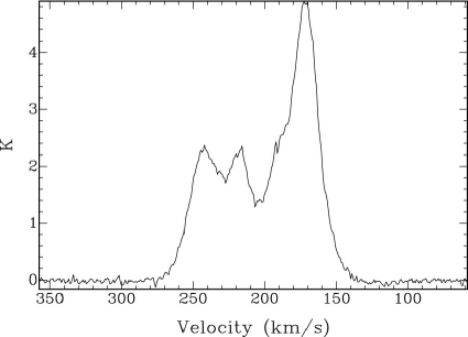
Figure 6: An example spectrum ($T_{\rm B}$ vs. $v_{\rm LSR}$) typical for the part of the Magellanic Bridge showing high velocity dispersions that is located at ($l$, $b$) = (290$\aas@@fstack{\circ}$52, –39$\aas@@fstack{\circ}$60). The 2nd moment of this spectrum is $\Delta v=30.5$ km s^-1, while the emission covers a velocity interval of about 125 km s^-1 (see Sect. 3.3).

3.3 Second Moment Analysis

The 2nd moment of an H i spectrum indicates the velocity spread of the H i gas within the velocity interval of interest. For a single cloud the 2nd moment is an indicator of its internal thermal and turbulent motions. However, within crowded regions like the Magellanic Clouds or the Magellanic Bridge, the 2nd moment can be considered as a measure of the relative velocity of individual clouds superposed on the same line-of-sight. The 2nd moment of a spectrum is calculated using

$$\Delta v=\sqrt{\frac{\Sigma(T_{{\rm B},i}\cdot(v_{i}-\overline{v})^{2})}{\Sigma T_{{\rm B},i}}},$$ (7)

where $T_{{\rm B},i}$ and $v_{i}$ indicate the brightness temperature and the radial velocity at channel $i$, respectively. $\overline{v}$ is the intensity weighted mean velocity calculated according to Eq. 3. Figure 4f shows the second moment map of the Magellanic Clouds and their environment. The averaged 2nd moment in the Magellanic Clouds and the Magellanic Bridge is $\Delta v\approx 20$ km s^-1 and covers the interval 10 km s${}^{-1}\leq\Delta v\leq 35$ km s^-1. The values for the Magellanic Bridge are significantly higher than those of the Magellanic Stream ($\Delta v\approx 15$ km s^-1) and the Leading Arm ($\Delta v\approx 8$ km s^-1). There are some lines-of-sight in the Interface Region with extremely high 2nd moments ($\Delta v\geq 45$ km s^-1), where multiple H i lines show extremely different radial velocities.

These high values for the Bridge are produced by superposed line profiles of clouds at different velocities (see Fig. 6). The individual line profiles show line widths comparable with those observed in the Magellanic Stream. The highest values of the 2nd moment correspond to the regions with the largest number of H i lines along the line-of-sight. They are located along the connecting line of both galaxies in the middle of the Bridge, where we also observe the highest column densities. Figure 5 shows that multiple components along the line-of-sight are very common in the Magellanic Bridge. Typical relative velocities of the individual line components within the Magellanic Bridge are of the order of 50 km s^-1, but some spectra show differences of up to 100 km s^-1.

Two clouds on the same line-of-sight having significantly different radial velocities must have different velocity vectors. Consequently, these two clouds will disperse if there is no restoring force keeping the clouds together. In the absence of a restoring force, the relative radial velocity gives an estimate of the increasing distance between these clouds. A velocity of 50 km s^-1 corresponds to a relative distance of 50 kpc after one Gyr. For comparison, the current relative distance of the Magellanic Clouds is approximately 20 kpc. A significant depth along the lines-of-sight through the Magellanic Bridge is therefore inevitable even if its age is significantly below one Gyr. However, the long-term stability of the Bridge is not clear, as indicated by the large amount of neutral hydrogen escaping towards the Interface Region (see Sect. 4.1).

3.4 H i masses

The Magellanic Clouds are embedded in a common H i envelope. Therefore, there is no obvious way to define borders between the LMC, the SMC, the Magellanic Bridge or the Interface Region. We used both column density and kinematical features to define a subdivision of the region around the Magellanic Clouds into complexes. Figure 4b shows the borders that separate the individual complexes.

The LMC and the SMC have within these borders total H i masses of $M$(H i) = (4.41$\pm$0.09)$\cdot$10⁸ M${}_{\odot}\left[d/50\leavevmode\nobreak\ {\rm kpc}\right]^{2}$ and $M$(H i) = (4.02$\pm$0.08)$\cdot$10⁸ M${}_{\odot}\left[d/60\leavevmode\nobreak\ {\rm kpc}\right]^{2}$, assuming optically thin emission and distances of 50 kpc and 60 kpc for the LMC and the SMC, respectively. The quoted uncertainties are two percent of the derived H i masses. They include residual baseline variations and calibration uncertainties. A larger error is introduced by the assumption of optically thin emission and the choice of the borders between the emission from the galaxies and the neighboring gas.

Staveley-Smith et al. (stavele2 (2003)) recently determined an H i mass of $M$(H i) = (4.8$\pm$0.2)$\cdot$10⁸ M${}_{\odot}\left[d/50\leavevmode\nobreak\ {\rm kpc}\right]^{2}$ for the LMC, also using the Parkes multi-beam facility. We derive a total H i mass of $M$(H i) = (4.6$\pm$0.1)$\cdot$10⁸ M_⊙ for the LMC, if we use the same borders between the emission from the LMC and the neighboring H i gas as Staveley-Smith et al. (stavele2 (2003)). The derived masses from both observations agree within their uncertainties.

Stanimirovic et al. (stanimirovic (1999)) derived an H i mass of $M$(H i) = (3.8$\pm$0.5)$\cdot$10⁸ M${}_{\odot}\left[d/60\leavevmode\nobreak\ {\rm kpc}\right]^{2}$ for the SMC, that is in good agreement with our value. Their mass increases to $M$(H i) = 4.2$\cdot$10⁸ M_⊙ after applying a self-absorption correction, indicating that the assumption of optically thin emission underestimates the true mass by about 10 percent.

The distances of the H i clouds outside the two galaxies are not well constrained by observations. Numerical simulations suggest that the matter in the Magellanic Bridge is located at similar distances than the Magellanic Clouds (e.g. Yoshizawa & Noguchi yoshizawa (2003)). Muller et al. (muller04 (2004)) analyzed the spatial power spectrum of the H i gas in the Magellanic Bridge and concluded that the Magellanic Bridge consists of two spatially and morphologically distinct components. As individual distances for these components are unknown a distance needs to be assumed to estimate the H i mass of the Magellanic Bridge. A reasonable estimate for the distance is the average of the distances of the LMC and the SMC, $d$ = 55 kpc. Using this distance and the borders defined above, the total H i mass of the Magellanic Bridge is $M$(H i) = 1.84$\cdot$10⁸ M${}_{\odot}\left[d/55\leavevmode\nobreak\ {\rm kpc}\right]^{2}$. The distance uncertainty dominates all other errors by at least one order of magnitude. The derived H i mass depends on distance quadratically. Increasing the distance estimate from 55 kpc to 60 kpc increases the derived mass by roughly 20 percent.

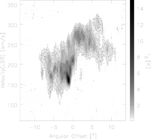
Figure 7: A position/velocity slice through the data-cube shown in Fig. 4 from ($l$,$b$) = (301$\aas@@fstack{\circ}$5, -30$\aas@@fstack{\circ}$5) to (274$\aas@@fstack{\circ}$0, -50$\aas@@fstack{\circ}$0). The position of this slice is marked in Fig. 4b by the dashed line B. Negative offset angles indicate emission from the Magellanic Bridge, positive ones emission from the Interface Region. Contour lines start at $T_{\rm B}$ = 0.15 K (3$\sigma$) and increase by factors of two, i.e. $T_{\rm B}$ = 0.3, 0.6, 1.2, 2.4, 4.8, and 9.6 K. The border between the Magellanic Bridge and the Interface Region is defined by the jump in the mean velocity at 0° angular offset.

4 The Interface Region and Isolated Clouds

4.1 The Interface Region

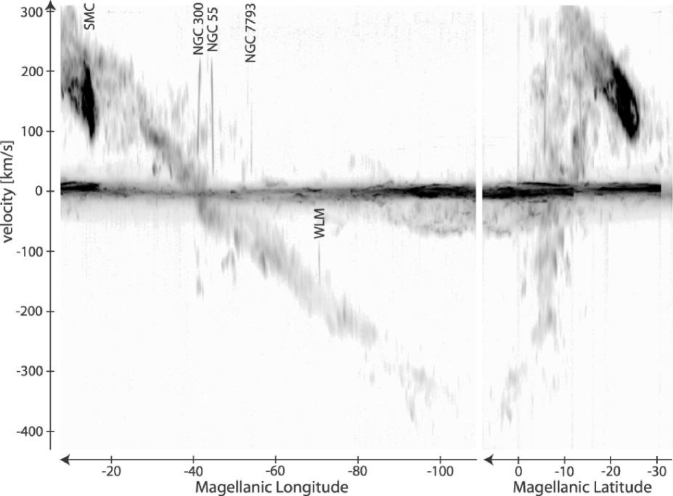
Figure 8: The two figures show position/velocity maps of the Magellanic Stream where the grey-scale represents the peak intensity along the third axis. Left: radial velocity ($v_{\rm LSR}$) is plotted as a function of Magellanic Longitude. The grey-scale indicates the peak intensity along the Magellanic Latitude axis of the data-cube (white corresponds to $T_{\rm B}=0$ K, black corresponds to $T_{\rm B}>20$ K). Right: radial velocity ($v_{\rm LSR}$) is plotted as a function of Magellanic Latitude. The grey-scale indicates the peak intensity along the Magellanic Longitude axis of the data-cube using the same grey-scale as in the left figure. The figures demonstrate that the Magellanic Stream forms an almost linear, coherent structure in the position-velocity space and covers a velocity interval between +250 km s^-1 and –400 km s^-1. Moreover, the maps show the emission from the SMC, the galaxies NGC 300, NGC 55, and NGC 7793 from the Sculptor Group, and the Local Group galaxy WLM. Some of the vertical lines, e.g. near Magellanic Latitude 0^∘, are produced by a higher noise close to the border of the mapped region.

The H i gas close to the SMC and the Magellanic Bridge shows a complex filamentary structure. This area (see Fig. 4b) will be called Interface Region henceforward. Most of these filaments point roughly towards the southern Galactic Pole. The high column density filament between Galactic longitude $l$ = 290^∘ and 300^∘ near $b\approx$ –55° is connected to the Magellanic Stream (Mathewson et al. mathewson (1974)) that continues towards the south passing the southern Galactic Pole (see Sect. 5).

The H i gas in the Interface Region has more positive velocities than the neighboring gas in the Magellanic Bridge. This difference in velocity is best visible in the LMC-standard-of-rest frame (Fig. 4e). Figure 7 shows a position/velocity slice through the data-cube shown in Fig. 4 from ($l$,$b$) = (301$\aas@@fstack{\circ}$5, -30$\aas@@fstack{\circ}$5) to (274$\aas@@fstack{\circ}$0, -50$\aas@@fstack{\circ}$0). This slice intersects both the Magellanic Bridge and the Interface Region. The discontinuity in the mean velocity (Fig. 7) was used to define a border between both complexes (compare Figs. 4b and e). The border between the Interface Region and the Magellanic Stream can be defined using the small gap near ($l$,$b$) = (300°, –61°).

The distances of the H i clouds in the Interface Region are not constrained by observations. Numerical simulations suggest distances of the clouds in this region between 30 and 80 kpc (e.g. Yoshizawa & Noguchi yoshizawa (2003)). As these simulations do not provide a one-to-one mapping of the Magellanic System, is it not possible to assign reliable distances to the individual complexes. A distance needs to be assumed for a comparison of the H i masses of the individual complexes. A reasonable estimate for this distance is 55 kpc, the average of the distances of the LMC and the SMC. Using this distance and the borders defined above (see Fig. 4b), the total H i mass of the Interface Region is $M$(H i) = 1.49$\cdot$10⁸ M${}_{\odot}\left[d/55\leavevmode\nobreak\ {\rm kpc}\right]^{2}$.

The huge amount of neutral hydrogen in the Interface Region, the alignment with the Magellanic Bridge and the smooth connection to the Magellanic Stream, both in position and in radial velocity, indicates that the Interface Region is closely related to the ongoing interaction of the Magellanic Clouds. The high velocity relative to the Magellanic Clouds (Fig. 4e) indicates that this material is currently leaving this region probably building a new section of the Magellanic Stream. The results suggest that the Magellanic Stream was most likely not created as a whole during a past encounter of the Magellanic Clouds, but is still in the continuous process of evolution (see also Putman et al. 2003a ).

Positive radial velocities, both relative to the Galactic-standard-of-rest and to the Magellanic Clouds, tend to indicate increasing distances and therefore higher orbits for the clouds in the Magellanic Stream. However, the space motion of the clouds outside the Magellanic Clouds is unknown and final conclusions about the three dimensional dynamics can only be made by comparing realistic numerical simulations with results from observations.

4.2 Isolated Clouds Close to the Magellanic Clouds

The H i on the northern boundary of the Bridge (in Galactic coordinates) appears much less structured than the H i in the Interface Region, although there are numerous clouds where the Magellanic Bridge adjoins the LMC near ($l$,$b$) $\approx$ (290^∘, –27^∘). This filament is part of the Leading Arm (Putman et al. 1998) and continues towards the Galactic Plane (see Sect. 6). The filament has a velocity of $v_{\rm LSR}\approx$ 300 km s^-1, comparable to the velocity of the Magellanic Bridge in this region.

There are also some clouds with lower radial velocities in this region. The largest cloud is located close to the LMC at ($l$,$b$) = (283$\degr$, –23$\aas@@fstack{\circ}$5). It shows an elongated structure and a radial velocity of $v_{\rm LSR}\approx$ 180 km s^-1 (see Fig. 4). In addition, there are two isolated clouds located near ($l$,$b$) = (304$\aas@@fstack{\circ}$5, –37$\aas@@fstack{\circ}$3) at $v_{\rm LSR}=110$ km s^-1 that were classified as compact high-velocity clouds (HVCs) by Putman et al. (putman4 (2002)). There are several compact and faint clouds at similar velocities close to the Magellanic Clouds and also on the same line-of-sight as the LMC (see Fig. 5). Some of these clouds have been detected in absorption against LMC stars (see Bluhm et al. bluhm (2001) and references therein). They must consequently have distances below 50 kpc (the distance of the LMC), indicating that they are foreground objects either of Magellanic origin or “normal” HVCs accidentally located in this region. The observed metallicities (Bluhm et al. bluhm (2001)) and the detection of molecular hydrogen (Richter et al. richterlmc (1999)) are consistent with a Magellanic origin, but a Galactic origin cannot be excluded.

The compact and isolated clouds in this region have typical peak column densities within the interval 2$\cdot$10¹⁹cm${}^{-2}\leq N$(H i) $\leq$ 5$\cdot$10¹⁹cm^-2. The low column densities involve a relatively low total H i mass associated with these clouds of $M$(H i) = 1.2$\cdot$10⁶ M${}_{\odot}\left[d/55\leavevmode\nobreak\ {\rm kpc}\right]^{2}$. A distance of 55 kpc was used for the H i mass to demonstrate that this gas does not affects the mass estimate of the LMC, the SMC, the Magellanic Bridge, or the Interface Region.

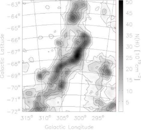
Figure 9: H i column density map of the high column density filament in the positive velocity part of the Magellanic Stream. The contour-lines indicate H i column densities of $N$(H i) = 1$\cdot$10¹⁹cm^-2 and $N$(H i) = 5$\cdot$10¹⁹cm^-2, further increasing in steps of $N$(H i) = 5$\cdot$10¹⁹cm^-2.

5 H i gas in the Magellanic Stream

5.1 The overall morphology

The Magellanic Stream is a $\approx$ 100° long coherent structure that is connected to the Interface Region (see Fig.  2 for an overview of the column density distribution). There is no clear starting point of the Magellanic Stream. We have defined a separation between the Interface Region and the Magellanic Stream near ($l$,$b$) = (300°, –61°).

The Magellanic Stream appears to be much more confined than the Interface Region. The data clearly show that a simple subdivision in six clouds MS I to MS VI (Mathewson et al. mathewson4 (1977)) is not appropriate with the current resolution and sensitivity. Figure 8 shows a peak intensity map of the Magellanic Stream in the position/velocity space, where radial velocity is plotted on the y-axis, while the position is plotted on the x-axis. This figure illustrates the distribution of the neutral hydrogen in the Magellanic Stream relative to Milky Way gas. The radial velocity changes dramatically over the extent of the Magellanic Stream starting at $v_{\rm LSR}\approx$ +250 km s^-1 near the Magellanic Bridge and decreasing to $v_{\rm LSR}\approx$ –400 km s^-1 near ($l$,$b$) = (90°, –45°), forming an almost linear structure in the position/velocity space. This velocity difference of $\Delta v_{\rm LSR}$ = 650 km s^-1 decreases to $\Delta v_{\rm GSR}$ = 390 km s^-1 in the Galactic-standard-of-rest frame. While the projection effect from the solar velocity vector explains a significant fraction of the velocity difference, the majority of the velocity gradient is related to the Magellanic Stream itself. The observed velocity gradient is inconsistent with a circular orbit of the Magellanic Stream. There are, however, various types of orbits that could explain the observed velocity gradient.

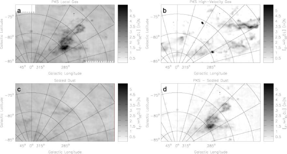
Figure 10: The maps show the region where the Magellanic Stream has radial velocities comparable to the local gas of the Milky Way. a) The H i column density integrated between $-40$ km s${}^{-1}\leq v_{\rm LSR}\leq+30$ km s^-1. b) The H i column density integrated between $-280$ km s${}^{-1}\leq v_{\rm LSR}\leq-40$ km s^-1 and $+30$ km s${}^{-1}\leq v_{\rm LSR}\leq+250$ km s^-1. c) The dust column density (Schlegel et al. schlegel (1998)) scaled to H i column densities. d) The difference map subtracting the column densities of map c from those of map a. The residual H i column density in this region is most likely associated with the Magellanic Stream.

The description of the Magellanic Stream in this section will be subdivided into four parts: H i gas at positive velocities, gas close to Galactic velocities and gas at low and high negative velocities.

5.2 The Magellanic Stream at positive velocities

The first part of the Magellanic Stream, also known as MS I, has positive radial velocities. This part of the Magellanic Stream comprises two parallel filaments and a number of smaller clouds close to the main filaments. The H i mass in this part of the Magellanic Stream is $M$(H i) = 4.3$\times$10⁷ M${}_{\odot}\left[d/55\leavevmode\nobreak\ {\rm kpc}\right]^{2}$.

The filament between ($l$,$b$) = (300°, –65.5°) and ($l$,$b$) = (308°, –70.5°) shows the highest column densities in the part of the Magellanic Stream that is not confused by Milky Way gas. The peak column density of $N$(H i) = 4.7$\cdot$10²⁰ cm^-2 is located at ($l$,$b$) = (301.5°, –67.7°) (see Fig. 9). The total H i mass of this filament (only the main filament without the neighboring clouds) is $M$(H i) = 1.4$\cdot$10⁷ M${}_{\odot}\left[d/55\leavevmode\nobreak\ {\rm kpc}\right]^{2}$. The H i mass of this filament is comparable to the mass of a very low-mass galaxy and about three times higher than the cloud close to M31 discovered by Davies (davies (1975)). This filament might represent the very early stage of a newly born dwarf galaxy. A detailed analysis of this filament will be presented in a separate paper.

5.3 The Magellanic Stream at Galactic velocities

The second part of the Magellanic Stream, also known as MS II, is difficult to analyze, because it shows radial velocities comparable to those of the local ISM of the Milky Way. Fortunately, this part of the Magellanic Stream is located close to the southern Galactic Pole, where the Milky Way shows low column densities. Figure 10a shows the H i column density of this region integrated between $-40$ km s${}^{-1}\leq v_{\rm LSR}\leq+30$ km s^-1. The H i gas in this region is relatively smoothly distributed with typical column densities of $N$(H i) = 1 to 2$\cdot$10²⁰ cm^-2, but there is a high column density region near ($l$,$b$) = (305$\aas@@fstack{\circ}$5, $-$79$\aas@@fstack{\circ}$5). Figure 10b shows the column density of the H i gas not confused by Galactic emission (integrated over $-280$ km s${}^{-1}\leq v_{\rm LSR}\leq-40$ km s^-1 and $+30$ km s${}^{-1}\leq v_{\rm LSR}\leq+250$ km s^-1). The region with high column densities is located exactly in that area where the Magellanic Stream shows velocities comparable to the local gas of the Milky Way. Figure 11 shows a spectrum of the position with the highest column density of $N$(H i) = 5.9$\cdot$10²⁰ cm^-2 at ($l$,$b$) = (305$\aas@@fstack{\circ}$5, $-$79$\aas@@fstack{\circ}$5). The line profiles of the Milky Way and the Magellanic Stream partly overlap.

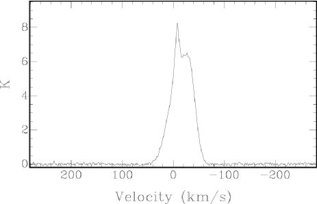
Figure 11: A spectrum ($T_{\rm B}$ vs. $v_{\rm LSR}$) of the line-of-sight with the highest column density in MS II at ($l$,$b$) = (305$\aas@@fstack{\circ}$5, $-$79$\aas@@fstack{\circ}$5). The local gas of the Milky Way has a velocity of $v_{\rm LSR}$ = $-$8 km s^-1, the Magellanic Stream has a velocity of $v_{\rm LSR}$ = $-$25 km s^-1.

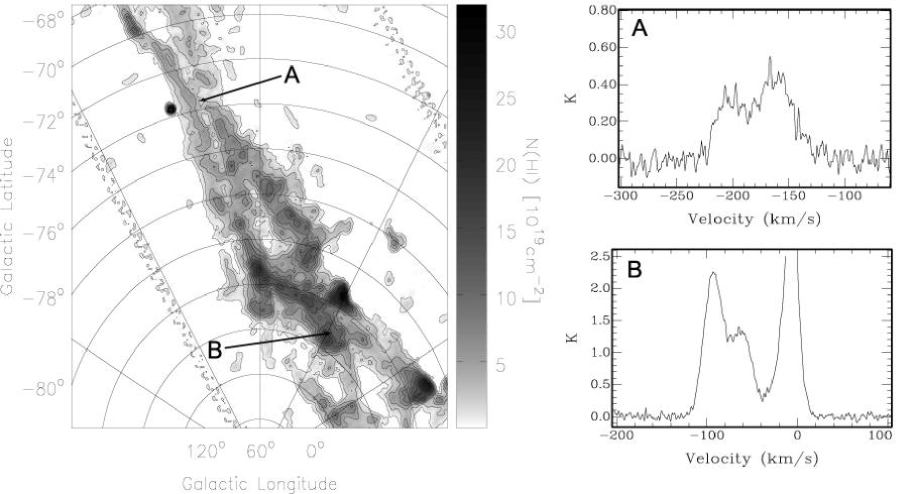
Figure 12: H i column density map of the part of the Magellanic Stream showing negative velocities. The contour-lines indicate H i column densities of $N$(H i) = 0.5$\cdot$10¹⁹cm^-2 and $N$(H i) = 2$\cdot$10¹⁹cm^-2, further increasing in steps of $N$(H i) = 2$\cdot$10¹⁹cm^-2. The two spectra show lines-of-sight where the two filaments of the Magellanic Stream are crossing. Spectrum A is located at ($l$,$b$) = (71$\aas@@fstack{\circ}$4, –73$\aas@@fstack{\circ}$5) and spectrum B at ($l$,$b$) = (29$\aas@@fstack{\circ}$4, –83$\aas@@fstack{\circ}$4). The two filaments have different radial velocities differing by $\Delta v\leavevmode\nobreak\ =\leavevmode\nobreak\ 41$ km s^-1 and $\Delta v\leavevmode\nobreak\ =\leavevmode\nobreak\ 31$ km s^-1 for spectra A and B.

Fong (fong (1987)) used IRAS data to demonstrate that there is no detectable dust emission associated with the Magellanic Stream. Schlegel et al. (schlegel (1998)) produced dust column density maps using IRAS and DIRBE data and found that there is a good correlation between H i column density and dust emission in low column density areas like the region close to the Galactic Poles. The non-detection of dust emission of the Magellanic Stream can be used to disentangle the column densities of the Milky Way and the Stream. We used the dust extinction maps from Schlegel et al. (schlegel (1998)), smoothed to the same angular resolution as the Parkes data, and regions without Magellanic emission to derive a linear correlation between the dust extinction and H i column density:

$$N({\rm{H\textsc{i}}})=6.85\cdot 10^{22}\leavevmode\nobreak\ {\rm cm}^{-2}\leavevmode\nobreak\ {\rm mag}^{-1}\leavevmode\nobreak\ E(B-V)+3.7\cdot 10^{20}\leavevmode\nobreak\ {\rm cm}^{-2}.$$ (8)

Figure 10c shows the dust emission map scaled to H i column densities using Eq. 8. Figure 10d shows the residual column density after subtracting the column densities from Fig. 10c from those of Fig. 10a. The residual column density corresponds to H i gas that is not traced by dust emission and is most likely associated with the Magellanic Stream. The regions that appear to be free from Magellanic emission show a 1-$\sigma$ rms noise of $N$(H i) $\approx$ 1.2$\cdot$10¹⁹ cm^-2. The map shows a bright peak with a column density of $N$(H i) = 4.8$\cdot$10²⁰ cm^-2 that corresponds to a 40-$\sigma$ detection. The emission of the Magellanic Stream has a peak intensity comparable to the local gas of the Milky Way, but a larger line width resulting in a larger column density. The total H i mass from the Magellanic Stream in this region, $M$(H i) = 4.3$\cdot$10⁷ M${}_{\odot}\left[d/55\leavevmode\nobreak\ {\rm kpc}\right]^{2}$, is comparable to the H i mass of the part of the Magellanic Stream presented in the previous section. Solely emission above the 3-$\sigma$ level was taken into account for the mass estimate. The estimated mass is therefore less accurate, because of the residual confusion with Milky Way emission.

5.4 The Magellanic Stream at negative velocities

The third part of the Magellanic Stream (MS III to MS IV) exhibits increasingly negative velocities. Figure 8 shows peak intensity maps in the position-velocity space. This part of the Magellanic Stream forms a continuous feature, having much lower intensities than the first two parts. The two filaments in this region (see Fig. 12) have a helix-like structure (see also Putman et al. 2003a ). The two spectra from Fig. 12 show positions where the two filaments are located on the same line-of-sight. The two filaments are clearly separated in velocity with radial velocities differing by $\Delta v=41$ km s^-1 (for spectrum A) and $\Delta v=31$ km s^-1 (for spectrum B). The three dimensional distribution of the gas cannot be derived from H i data alone. Nevertheless, the helical structure might indicate the footprint of the Magellanic Clouds, while rotating around each other in the past, consistent with a continuous stripping of gas from the Magellanic Bridge as indicated in Sect. 3.2. The angular width of the filaments is decreasing towards more negative velocities. The highest column density of $N$(H i) = 3.1$\cdot$10²⁰ cm^-2 is located at ($l$,$b$) = (31.2°, –81.5°). This cloud shows more negative velocities ($\Delta v_{\rm LSR}=20$ km s^-1) than the neighboring clouds in the main filament of the Magellanic Stream, but it is smoothly connected with the main stream showing a continuous velocity gradient. The cloud has an H i mass of $M$(H i) = 1.4$\cdot$10⁶ M${}_{\odot}\left[d/55\leavevmode\nobreak\ {\rm kpc}\right]^{2}$. The total H i mass of the third part of the Stream, south of $b$ = –70°, is $M$(H i) = 3.0$\cdot$10⁷ M${}_{\odot}\left[d/55\leavevmode\nobreak\ {\rm kpc}\right]^{2}$. The clouds in this part of the Stream have line-widths of the order of $\Delta v_{\rm FWHM}$ = 30 – 35 km s^-1.

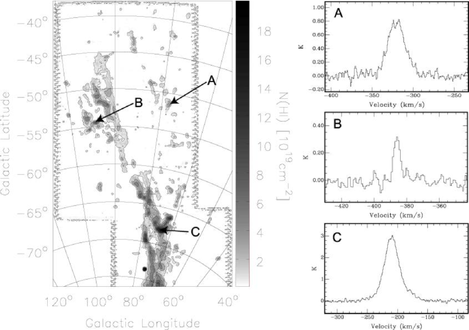
Figure 13: H i column density map of the part of the Magellanic Stream showing high negative velocities. The contour-lines indicate H i column densities of $N$(H i) = 0.5$\cdot$10¹⁹cm^-2 and $N$(H i) = 2$\cdot$10¹⁹cm^-2, further increasing in steps of $N$(H i) = 2$\cdot$10¹⁹cm^-2. Three exemplary spectra located at ($l$,$b$) = (78$\aas@@fstack{\circ}$6, –51$\aas@@fstack{\circ}$6), (93$\aas@@fstack{\circ}$6, –53$\aas@@fstack{\circ}$7), and (73$\aas@@fstack{\circ}$4, –68$\aas@@fstack{\circ}$0) are shown to the left. These H i lines are well represented by single Gaussians with line widths of $\Delta v_{\rm FWHM}$ = 23 km s^-1, $\Delta v_{\rm FWHM}$ = 3.9 km s^-1, and $\Delta v_{\rm FWHM}$ = 28 km s^-1 for spectra A, B, and C, respectively.

5.5 The Magellanic Stream at high negative velocities

The last section of the Magellanic Stream (MS IV to MS VI) has very high negative radial velocities (up to $v_{\rm LSR}$ = –400 km s^-1) and low column densities. Figure 13 shows the column density distribution of this part of the Magellanic Stream. The cloud located at ($l$,$b$) = (73.5°, –68°) has a horse-shoe like shape and asymmetric line-profiles with wings in direction towards less negative velocities. The Stream fans out into numerous curved filaments and isolated clouds north of this cloud. Sembach et al. (sembach2 (2003)) detected O vi absorption associated with the Magellanic Stream. They detected also O vi absorption at similar velocities along sight-lines where no H i emission has been detected to far. These detections indicate that the ionized component of the Magellanic Stream is more extended than the neutral gas. The total H i mass of this part of the Stream, $b\geq$ –70°, is $M$(H i) = 0.9$\cdot$10⁷ M${}_{\odot}\left[d/55\leavevmode\nobreak\ {\rm kpc}\right]^{2}$. The mass of the ionized component is not well constrained by observations.

The H i gas in the very-high-velocity part of the Magellanic Stream has typical line-widths in the range $\Delta v_{\rm FWHM}$ = 20 – 35 km s^-1 (see Fig. 13, spectra A and C). The cloud located at ($l$,$b$) = (94.5°, –54.5°) is of particular interest: it shows more negative velocities than the neighboring clouds, it has a peak column density of $N$(H i) = 6$\cdot$10¹⁹ cm^-2 and specifically, the profile shows two distinct components. One with a line-width that is normal for the Magellanic Stream and one component with a surprisingly narrow line-width. The lowest line width of $\Delta v_{\rm FWHM}\approx$ 4 km s^-1 (Fig. 13, spectrum B) is observed at the northern edge of this cloud at ($l$,$b$) = (93$\aas@@fstack{\circ}$6, –53$\aas@@fstack{\circ}$7). The line-width allows to derive an upper limit for the temperature of $T_{D}$ = 21.8$\cdot\Delta v^{2}_{\rm FWHM}$ = 350 K. The kinetic temperature of the H i gas must be lower, as turbulent motions also broaden the line. This cloud proves the existence of a cool gas phase in the Magellanic Stream.

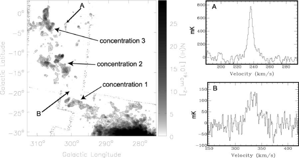
Figure 14: H i column density map of the very-high-velocity clouds close to the LMC integrated over the velocity interval 150 km s${}^{-1}\leavevmode\nobreak\ \leq\leavevmode\nobreak\ v_{\rm LSR}\leavevmode\nobreak\ \leq$ 420 km s^-1 for $b\leq$ –10° and 180 km s${}^{-1}\leavevmode\nobreak\ \leq\leavevmode\nobreak\ v_{\rm LSR}\leavevmode\nobreak\ \leq$ 420 km s^-1 for $b>$ –10° to exclude emission from the Galactic Plane. The contour-lines indicate H i column densities of $N$(H i) = 0.5$\cdot$10¹⁹cm^-2 and $N$(H i) = 2$\cdot$10¹⁹cm^-2, further increasing in steps of $N$(H i) = 2$\cdot$10¹⁹cm^-2. The spectrum A shows a compact cloud at ($l$,$b$) = (300$\aas@@fstack{\circ}$6,–3$\aas@@fstack{\circ}$1) with a FWHM line width of $\Delta v$ = 6 km s^-1. The spectrum B, located at ($l$,$b$) = (300$\aas@@fstack{\circ}$3,–20$\aas@@fstack{\circ}$3), indicates that there is faint emission connecting the main concentrations of the complex LA I. This spectrum is located on a line-of-sight where two observed fields overlap leading to a $\sqrt{2}$ lower noise of this spectrum.

5.6 Isolated Clouds towards the Sculptor Group

Figure 8 shows the Magellanic Stream clouds and the galaxies NGC 55, NGC 300, and NGC 7793, having distances of 1.6 Mpc, 2.1 Mpc, and 3.4 Mpc, respectively (Cote et al. cote (1997)). These galaxies form the near part of the Sculptor group. The two galaxies NGC 55 and NGC 300 fall exactly onto the line-of-sight to the Magellanic Stream. They have radial velocities of the order of $v_{\rm LSR}$ = 100 km s^-1, while the main filament of the Magellanic Stream has velocities in the interval –30 km s${}^{-1}\leq v_{\rm LSR}\leq$ 30 km s^-1 at that position. The galaxies NGC 55 and NGC 300 are easy to identify, as they have high intensities and a large extent in velocity. There are a number of small clouds in this region having high positive velocities deviating up to $\Delta v\approx$ 200 km s^-1 from the main filament of the Magellanic Stream. The enormous scatter of radial velocities near Magellanic longitude $L_{\rm M}$ = –50°  is nicely visible in Fig. 8. NGC 55 is located at Magellanic longitude $L_{\rm M}$ = –49.2°  and NGC 300 at $L_{\rm M}$ = –47.3°. The small H i clouds in this region are located in the same region on the sky as the galaxies NGC 55 and NGC 300 showing similar velocities. Mathewson et al. (mathewson2 (1975)) suggested that these clouds are located within the Sculptor group, but Haynes & Roberts (haynes2 (1979)) found that the overall distribution and kinematics of these clouds do not fit to the Sculptor group. Numerous possible origins of these clouds have been discussed in the literature (see Putman et al. 2003a and references therein). Recently, Bouchard et al. (bouchard (2003)) argued that some of these clouds might be associated with the Sculptor dSph galaxy that is located close to the Magellanic Stream at ($l$,$b$) = (287$\aas@@fstack{\circ}$53, –83$\aas@@fstack{\circ}$16).

6 H i gas in the Region of the Leading Arm

Figure 2 shows, next to the Magellanic Clouds and the Magellanic Stream, the H i column density distribution of very-high velocity clouds north of the LMC. The very-high-velocity gas in Fig. 2 represents the majority of the population EP high-velocity clouds (see Wakker & van Woerden wvw (1991)).

The very-high-velocity clouds can be grouped into three complexes. First, a complex that is located between the Magellanic Clouds and the Galactic Plane. This complex was discovered by Mathewson et al. (mathewson (1974)). Second, a $\approx$25° long filament (285°$\leq l\leq$ 295°, 0° $<b<$ 30°), that is part of HVC-complex WD (Wannier et al. wannier2 (1972)). Third, a complex (265° $\leq l\leq$ 280°, 0° $<b<$ 30°), that is also part of HVC-complex WD. The three complexes will be called LA I, LA II, and LA III henceforward.

6.1 Complex LA I

The complex LA I starts close to the LMC and ends at the Galactic Plane near $l$ = 305$\aas@@fstack{\circ}$5. It was discovered by Mathewson et al. (mathewson (1974)) and studied in more detail by Mathewson et al. (mathewson3 (1979)), Morras (morrasa (1982)), and Bajaja et al. (bajaja (1989)).

Figure 14 shows a H i column density map of the complex LA I. The complex does not appear as one coherent stream, but comprises three main concentrations with a high column density and a number of faint, compact clouds.

The first concentration forms a linear structure with several small clouds between ($l$,$b$) = (293^∘, –25^∘) and (301^∘, –22^∘) that is directly connected with the H i clouds close to the LMC, both in position and in radial velocity (see also Fig. 4). The peak column density is $N$(H i) = 6.9$\cdot$10¹⁹cm^-2 and the total H i mass is $M$(H i) = 1.2$\cdot$10⁶ M${}_{\odot}\left[d/55\leavevmode\nobreak\ {\rm kpc}\right]^{2}$. The radial velocities are in the range 230 km s^-1 $\leq\leavevmode\nobreak\ v_{\rm LSR}\leq$ 330 km s^-1. Typical line-widths are in the range 20 km s^-1 $\leq\leavevmode\nobreak\ \Delta v_{\rm FWHM}\leavevmode\nobreak\ \leq$ 30 km s^-1.

The second concentration consists of three big clouds surrounded by a number of compact clouds. This concentration is connected with the one close to the LMC by a very faint filament (see Fig. 14). Two of the big clouds show a rather diffuse column density distribution with radial velocities of about $v_{\rm LSR}\approx$ 300 km s^-1. The third big cloud has a radial velocity of $v_{\rm LSR}\approx$ 245 km s^-1. This cloud shows the highest column density ($N$(H i) = 1.6$\cdot$10²⁰cm^-2) of LA I. The cloud is much more concentrated with a steep column density gradient at the border. The total H i mass of these three clouds is $M$(H i) = 3.8$\cdot$10⁶ M${}_{\odot}\left[d/55\leavevmode\nobreak\ {\rm kpc}\right]^{2}$.

The third concentration is connected with the second one by a number of faint clouds (see Fig. 14). This concentration is a 5^∘ long and 1^∘ wide complex that is orientated perpendicular to the Galactic Plane. The radial velocities of this filament vary from $v_{\rm LSR}\approx$ 250 km s^-1 to $v_{\rm LSR}\approx$ 220 km s^-1 near the Galactic Plane. There is a 5^∘ long low column density feature at $b\approx$ –3^∘, that is orientated parallel to the Galactic Plane. The third part of LA I has a peak column density of $N$(H i) = 1.4$\cdot$10²⁰cm^-2 and a total H i mass of $M$(H i) = 4.4$\cdot$10⁶ M${}_{\odot}\left[d/55\leavevmode\nobreak\ {\rm kpc}\right]^{2}$. The high column density regions show line widths of about $\Delta v_{\rm FWHM}\approx$ 30 km s^-1, while the gas at the northern end of this section (that overlaps with the Galactic Plane) has relatively low line-widths in the range 5 km s^-1 $\leq\leavevmode\nobreak\ \Delta v_{\rm FWHM}\leavevmode\nobreak\ \leq$ 10 km s^-1. A line-width of $\Delta v_{\rm FWHM}\approx$ 5 km s^-1 gives an upper limit to the kinetic temperature of $T_{\rm D}$ = 545 K. The clouds near the Galactic Plane appear to be colder or less turbulent than other clouds in LA I.

The steep column density drop off and the narrow line widths close to the Galactic Plane can be interpreted as indication for a ram-pressure interaction with an ambient medium (Quilis & Moore quilis (2001); Konz et al. konz (2002)). The radial velocity of the fastest (and therefore most distant) component of the Galactic Disk at this position ($l\approx$ 305°) is $v_{\rm LSR}$ = 122 km s^-1. Extrapolating the rotation curve from Brand & Blitz (brand (1993)) yields a distance of $d\approx$ 30 kpc to the outermost spiral arm of the Milky Way (McClure-Griffiths et al. mcclure (2004)). It is expected that some diffuse, low density gas exists even beyond $d\approx$ 30 kpc. Recent n-body simulations predict a distance between 30 to 40 kpc to the Leading Arm in this region (see Fig. 2 of Gardiner gardiner (1999) or Fig. 11 of Yoshizawa & Noguchi yoshizawa (2003)). The comparable distances suggest a ram-pressure interaction between the Leading Arm and the gas in the very outer regions of the Galactic Disk.

The total H i mass of the three main concentrations of LA I is $M$(H i) = 9.4$\cdot$10⁶ M${}_{\odot}\left[d/55\leavevmode\nobreak\ {\rm kpc}\right]^{2}$. The main concentrations of LA I are accompanied by a number of small clouds with similar velocities (see Fig. 14).

There are some compact and isolated clouds located between 294^∘ $\leq l\leq$ 298^∘ that have radial velocities in the interval 300 km s^-1 $\leq v_{\rm LSR}\leq$ 350 km s^-1. The region between the Galactic Plane and $b$ = –20° and $l\leq$ 295° was not covered by this survey (see Fig. 2). Putman et al. (putman4 (2002)) found a number of compact clouds at similar velocities in this region using HIPASS data. The radial velocities of these clouds are comparable to those observed in the LMC and the complex LA II, but they do not fit to the neighboring gas of LA I.

6.2 Complex LA II

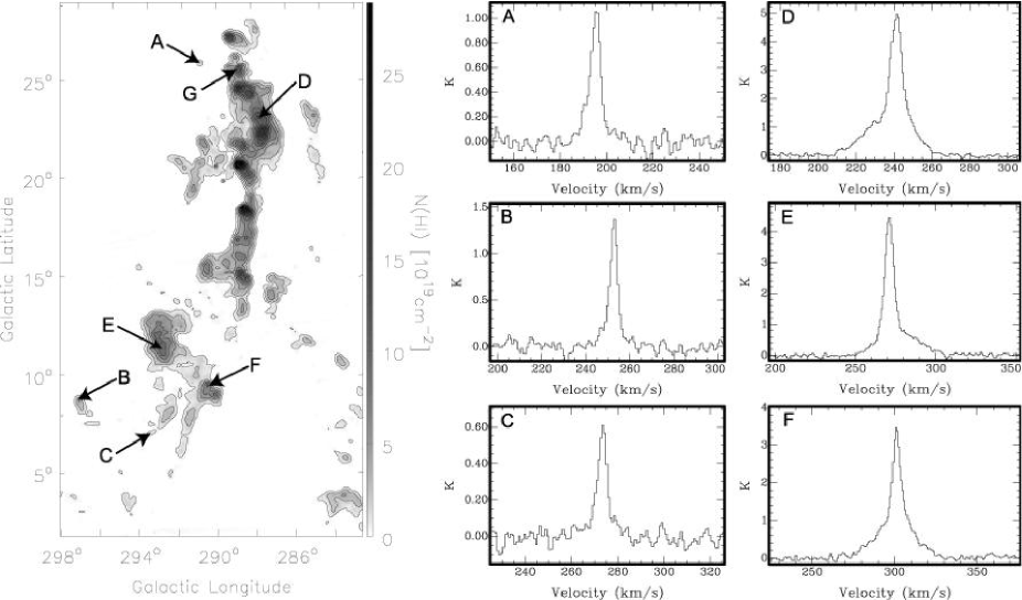
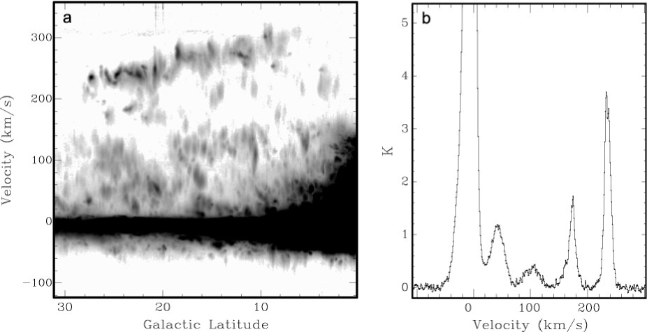
Figure 15: H i column density map of the very-high-velocity clouds in the complex LA II integrated over the velocity interval 175 km s${}^{-1}\leavevmode\nobreak\ \leq\leavevmode\nobreak\ v_{\rm LSR}\leavevmode\nobreak\ \leq$ 325 km s^-1. The contour-lines indicate H i column densities of $N$(H i) = 0.5$\cdot$10¹⁹cm^-2 and $N$(H i) = 2$\cdot$10¹⁹cm^-2, increasing in steps of $N$(H i) = 2$\cdot$10¹⁹cm^-2. The positions of the exemplary spectra A to F are ($l$,$b$) = (290$\aas@@fstack{\circ}$9,26$\aas@@fstack{\circ}$1), (297$\aas@@fstack{\circ}$3,8$\aas@@fstack{\circ}$9), (293$\aas@@fstack{\circ}$6,7$\aas@@fstack{\circ}$1), (287$\aas@@fstack{\circ}$7,23$\aas@@fstack{\circ}$3), (293$\aas@@fstack{\circ}$1,12$\aas@@fstack{\circ}$1), and (290$\aas@@fstack{\circ}$6,9$\aas@@fstack{\circ}$7), respectively. The spectra A, B, and C show narrow lines with a FWHM line width of $\Delta v$ = 5.3 km s^-1, $\Delta v$ = 4.1 km s^-1, and $\Delta v$ = 4.8 km s^-1, respectively. The spectra D, E, and F show examples of spectra with two components: a narrow and a broad line. The Gaussian decomposition yields line widths for the two components of $\Delta v$ = 6.7 km s^-1 and $\Delta v$ = 28.4 km s^-1 for spectrum D, $\Delta v$ = 6.4 km s^-1 and $\Delta v$ = 29.0 km s^-1 for spectrum E, and $\Delta v$ = 5.4 km s^-1 and $\Delta v$ = 26.2 km s^-1 for spectrum F. In some clouds of this complex the two components show slightly different velocities (e.g. spectra D and E).

Figure 16: a) Peak intensity position/velocity map of the complex LA II, representing the maximum brightness temperature along the Galactic Longitude axis. The grey-scale has a square root scaling from $T_{\rm B}$ = 0 K (white) to 10 K (black). The complex LA II appears as a continuous, linear feature with a velocity gradient from about $v_{\rm LSR}$ = 310 km s^-1 close to the Galactic Plane to $v_{\rm LSR}$ = 230 km s^-1 at its northern end. b) An example spectrum towards ($l$,$b$) = (288$\aas@@fstack{\circ}$78,26$\aas@@fstack{\circ}$65) that is marked with a “G” in Fig. 16. The spectrum shows multiple components covering the entire velocity interval between $v_{\rm LSR}$ = –50 km s^-1 and $v_{\rm LSR}$ = +260 km s^-1.

Complex LA II is located at 285°$\leq l\leq$ 295°, 0° $<b<$ 30° (see Fig. 16). It is part of HVC-complex WD (Wannier et al. wannier2 (1972)) and has been studied by several groups, e.g. Morras & Bajaja (morrasbajaja (1983)), and Wakker et al. (wakker2 (2002)).

The complex LA II consists of two parts. The first part is a 15° long, linear filament between 13° $\leq b\leq$ 28°. It comprises 11 high column density clouds ($N$(H i) $\geq$ 1$\cdot$10²⁰cm^-2) that are not resolved by the Parkes beam. The highest column density of $N$(H i) = 2.9$\cdot$10²⁰cm^-2, is located at ($l$,$b$) = (288.8°, 20.8°). The second part consists of a complex of clouds in the area 290° $\leq l\,\leq$ 295° and 5° $\leq\leavevmode\nobreak\ b\leavevmode\nobreak\ \leq$ 13° (Fig. 16). Both parts are connected by a bridge of very faint gas. The total H i mass of LA II is $M$(H i) = 1.1$\cdot$10⁷ M${}_{\odot}\left[d/55\leavevmode\nobreak\ {\rm kpc}\right]^{2}$.

The radial velocities of complex LA II start at $v_{\rm LSR}\leavevmode\nobreak\ \approx$ 310 km s^-1 close to the Galactic Plane and decrease to $v_{\rm LSR}\leavevmode\nobreak\ \approx$ 230 km s^-1 towards $b\approx$ 30° (Fig. 16a). This velocity gradient is slightly lower in the Galactic-standard-of-rest frame: from $v_{\rm GSR}\leavevmode\nobreak\ \approx$ 105 km s^-1 to $v_{\rm GSR}\leavevmode\nobreak\ \approx$ 45 km s^-1.

Close to the main filament there are a number of compact clouds with line widths down to $\Delta v_{\rm FWHM}\approx$ 4 km s^-1 (Fig. 16, spectra A, B, and C), indicating gas with temperatures below 350 K. Some clouds show two components in the spectra, a narrow and a broad line, indicating a warm and a cold gas-phase (Fig. 16, spectra D, E, and F). The broad component shows line widths of the order of $\Delta v_{\rm FWHM}\approx$ 25 km s^-1, indicating gas with temperatures below $T_{\rm D}\leq$ 14 000 K, while the typical line widths of the cold component are of the order of $\Delta v_{\rm FWHM}\approx$ 7 km s^-1, indicating gas with temperatures below $T_{\rm D}\leq$ 1000 K. A similar morphology has also been observed for several HVC-complexes (see Wakker & van Woerden wvwrev (1997) and references therein).

Wakker et al. (wakker2 (2002)) observed the cloud in the line-of-sight to NGC 3783 at ($l$,$b$) = (287$\aas@@fstack{\circ}$5, 22$\aas@@fstack{\circ}$5) in H i with high angular resolution using the ATCA. They detected numerous small, dense, and cold cores ($T_{\rm k}<$ 500 K) that are embedded in a smoother H i envelope.

Some clouds close to the Galactic Plane show a head-tail structure. These clouds have a high column density head with a narrow and a broad line component and a diffuse tail showing solely a broad component. Figure 17 shows one example of a cloud with an asymmetric column density distribution, a so-called head-tail structure (Brüns et al. bruens1 (2000); Brüns et al. bruens2 (2001)). The position/velocity slice through this cloud (Fig. 17b) shows that there is only a narrow component visible at the northern edge of the cloud ($\Delta v\approx$ 4 km s^-1), while there are two components detected in the middle part of that cloud and only a broad component towards the southern end ($\Delta v\approx$ 20 km s^-1). This morphology is suggestive of a ram-pressure interaction, where the diffuse gas (represented by the broad line) is stripped from the cold core (represented by the narrow line). This interpretation is supported by the numerical simulations from Quilis & Moore (quilis (2001)) and Konz et al. (konz (2002)). In the context of these simulations, this cloud would move northwards through an ambient medium.

Figure 16a shows that there are a number of compact clouds with radial velocities that are about 60 km s^-1 lower than those of the complex LA II. One example is a compact HVC with a diameter of about 40′ centered on ($l$,$b$) = (288$\aas@@fstack{\circ}$78, 26$\aas@@fstack{\circ}$65). Figure 16b shows a spectrum of this line-of-sight. The compact cloud has a velocity of $v_{\rm LSR}$ = 170 km s^-1, approximately 60 km s^-1 lower than the velocity of the LA II, but about 60 km s^-1 higher than the extended emission at $v_{\rm LSR}$ = 110 km s^-1 in this region.

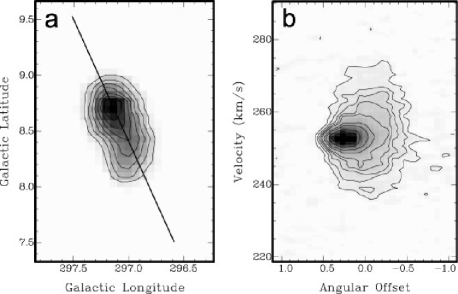
Figure 17: a) H i column density map of a head-tail cloud (cloud B in Fig. 16). The contour lines start at $N$(H i) = 0.5$\cdot$10¹⁹cm^-2 and increase in steps of $N$(H i) = 0.5$\cdot$10¹⁹cm^-2. The line shows the position of the slice shown in Fig. 17b. b) A position/velocity slice through the data-cube presented in Fig. 17a. Positive angular offsets are in direction of increasing Galactic Latitude. The contour lines represent brightness temperatures of $T_{\rm B}$ = 0.1, 0.2, 0.3, 0.4, 0.5, 0.75, 1.0, 1.5, and 2.0 K. Near offset angle +0$\aas@@fstack{\circ}$5 only a narrow component is visible in the spectra, near offset angle +0$\aas@@fstack{\circ}$2 a narrow and a broad line are detected, and near offset angle –0$\aas@@fstack{\circ}$25 only a broad line is visible.

The H i emission around $b\approx$ 25° at $v_{\rm LSR}$ = 110 km s^-1 and the emission between 10° $\leq b\leq$ 20° at $v_{\rm LSR}$ = 120 km s^-1 show a high velocity relative to the local gas of the Milky Way, but they are nevertheless no HVCs. Wakker (wakkerdev (1991)) defined HVCs as clouds with radial velocities that deviate by at least 50 km s^-1 from those velocities expected from Galactic rotation at their position. The radial velocity of the fastest (and therefore most distant) component of the Galactic Disk shows similar velocities of the order $v_{\rm LSR}\approx$ 120 km s^-1. These velocities imply a distance of $d\approx$ 30 kpc (Brand & Blitz brand (1993)). The clouds with $b\geq$ 5° can therefore be interpreted as co-rotating Galactic H i clouds at a distance of $d\approx$ 30 kpc that are located at z-heights of 5 to 10 kpc above the Galactic Disk. The kinematical distance, however, is only an estimate as the assumption of co-rotation is not necessarily true for these clouds.

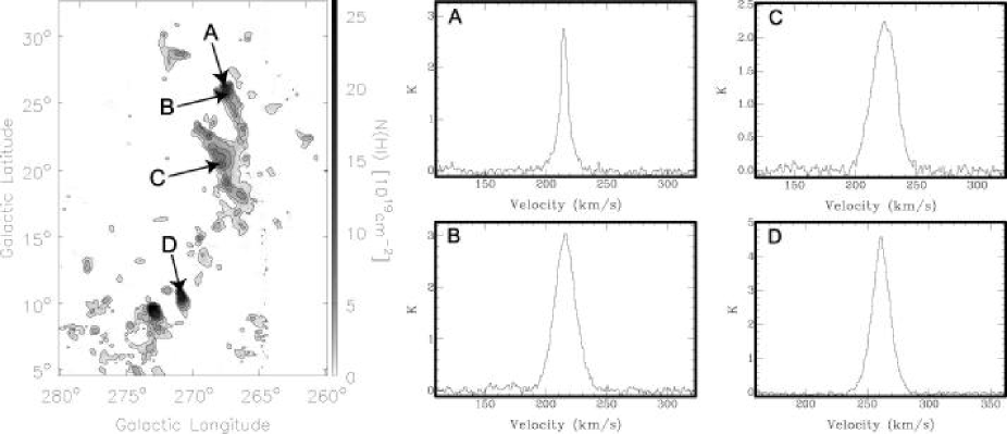
Figure 18: H i column density map of the very-high-velocity clouds in the complex LA III integrated over the velocity interval 170 km s${}^{-1}\leavevmode\nobreak\ \leq\leavevmode\nobreak\ v_{\rm LSR}\leavevmode\nobreak\ \leq$ 300 km s^-1. The contour-lines indicate H i column densities of $N$(H i) = 0.5$\cdot$10¹⁹cm^-2 and $N$(H i) = 2$\cdot$10¹⁹cm^-2, increasing in steps of $N$(H i) = 2$\cdot$10¹⁹cm^-2. The cloud at ($l$,$b$) = (267^∘, 26^∘) shows a steep column density gradient on one side and an extended tail on the opposite side. Spectrum A is located at the steep gradient, ($l$,$b$) = (267$\aas@@fstack{\circ}$5, 26$\aas@@fstack{\circ}$7). It shows two components with FWHM line widths of $\Delta v$ = 4.4 km s^-1 and $\Delta v$ = 15.2 km s^-1. Spectrum B shows the same cloud, but on the side towards the tail, ($l$,$b$) = (267$\aas@@fstack{\circ}$2, 26$\aas@@fstack{\circ}$0). The line is well represented by a single Gaussian with a line width of $\Delta v$ = 20.2 km s^-1. The spectra C and D are located at ($l$,$b$) = (267$\aas@@fstack{\circ}$8, 20$\aas@@fstack{\circ}$7) and ($l$,$b$) = (271$\aas@@fstack{\circ}$0, 11$\aas@@fstack{\circ}$1). They show lines with a line width of $\Delta v$ = 22.9 km s^-1 and $\Delta v$ = 17.3 km s^-1, respectively.

6.3 Complex LA III

Figure 18 shows the H i column density distribution of the complex LA III that is also part of the HVC-complex WD (Wannier et al. wannier2 (1972)). The complex LA III is approximately parallel to LA II, but shifted towards lower Galactic longitudes (265°$\leq l\leq$ 280°). LA III is not as continuous as LA II: there are two high column density clouds close to the Galactic Plane ($b\approx$ 10°), first studied by Morras & Bajaja (morrasbajaja (1983)), and a larger cloud complex (12° by 5°) centered on ($l$,$b$) = (267°, +22°). These clouds have been studied in H i by Giovanelli & Haynes (giovanelli (1976)) and Cavarischia & Morras (cavarischia (1989)).

The two bright clouds close to the Galactic Plane at ($l$,$b$) = (273$\aas@@fstack{\circ}$0, 9$\aas@@fstack{\circ}$9) and ($l$,$b$) = (270$\aas@@fstack{\circ}$8, 10$\aas@@fstack{\circ}$7) have peak column densities of $N$(H i) = 2.9$\cdot$10²⁰cm^-2 and $N$(H i) = 1.7$\cdot$10²⁰cm^-2, and mean velocities of $v_{\rm LSR}$ = 248 km s^-1 and $v_{\rm LSR}$ = 259 km s^-1, respectively. There are numerous low column density clouds with similar radial velocities in this region, especially close to the Galactic Plane. The highest radial velocity of $v_{\rm LSR}$ = 279 km s^-1 is observed at ($l$,$b$) = (271$\aas@@fstack{\circ}$9, 11$\aas@@fstack{\circ}$3). The velocities are within 210 km s${}^{-1}\leq v_{\rm LSR}\leq$ 230 km s^-1 for the complex centered on ($l$,$b$) = (267°, +22°) and $v_{\rm LSR}$ = 185 km s^-1 for the cloud at ($l$,$b$) = (271°, +29°). The total H i mass of clouds in the area of LA III is $M$(H i) = 8.1$\cdot$10⁶ M${}_{\odot}\left[d/55\leavevmode\nobreak\ {\rm kpc}\right]^{2}$.

Typical line widths in this complex cover the interval 20 km s^-1 $\leq\Delta v_{\rm FWHM}\leq$ 30 km s^-1 (see Fig. 18). These values are comparable to the broad component observed in LA II. A narrow component has been observed solely for the cloud centered at ($l$,$b$) = (267^∘, 26^∘). It shows a steep column density gradient on one side and an extended tail on the opposite side, forming a head-tail structure. Spectrum A of Fig. 18 is located at the steep gradient. It shows two components with FWHM line widths of $\Delta v$ = 4.4 km s^-1 and $\Delta v$ = 15.2 km s^-1. Spectrum B of Fig. 18 shows the same cloud, but on the side towards the tail. The line is well represented by a single Gaussian with a line width of $\Delta v$ = 20.2 km s^-1.

The cloud at ($l$,$b$) = (270$\aas@@fstack{\circ}$8, 10$\aas@@fstack{\circ}$7) also shows an elongated structure with line widths increasing from its northern end ($\Delta v_{\rm FWHM}\approx$ 15 km s^-1) to its southern end ($\Delta v_{\rm FWHM}\approx$ 25 km s^-1).

6.4 Discussion of the H i in the Leading Arm Region

The complexes LA I, LA II, and LA III have already been associated with the Magellanic Clouds by Mathewson et al. (mathewson (1974)). However, two arguments have been used to disprove the association with the Magellanic Clouds: first, the morphological differences between the Magellanic Stream and the Leading Arm, especially the existence of a two-phase medium in the Leading Arm, and second the absence of a clear velocity gradient of the Leading Arm (e.g. Morras morrasa (1982)).

The morphological differences between the neutral hydrogen in the Leading Arm and the Magellanic Stream include a different distribution of the gas (a coherent stream in case of the Magellanic Stream and clumpy filaments in case of the Leading Arm) and the unequal types of line profiles (the H i lines show a narrow and a broad component for numerous clouds in the Leading Arm and only one broad component in the Magellanic Stream). Recent numerical simulations suggest that the distance to the Magellanic Stream is considerably larger than the distance to the Leading Arm (Gardiner gardiner (1999); Yoshizawa & Noguchi yoshizawa (2003); Connors et al. connors (2004)). Moreover, the Magellanic Stream is located at high Galactic latitudes implying large distances from the Galactic Plane. In contrast, the Leading Arm is located at low Galactic latitudes. The expected distance to the Leading Arm is consistent with the distance to the outermost parts of the Galactic Disk (see Sect. 6.1). The density of the ambient medium of the Leading Arm is therefore expected to be much higher than the density of the medium close to the Magellanic Stream. Wolfire et al. (wolfire (1995)) demonstrated that the existence of two stable gas phases depends strongly on the pressure of the ambient medium. The morphological differences of the gas in the Leading Arm and the gas in the Magellanic Stream might therefore be a product of different environmental conditions. Consequently, the presence of two gas phases does not argue against a common Magellanic origin of the complexes LA I, LA II, and LA III.

The Magellanic Stream shows a velocity gradient of $\Delta v_{\rm LSR}$ = 650 km s^-1 and $\Delta v_{\rm GSR}$ = 390 km s^-1 in the Galactic-standard-of-rest frame (see Sect. 5.1), while clouds in the Leading Arm do not show a clear velocity gradient (Fig. 3). Recent numerical simulations of the Magellanic System (Gardiner gardiner (1999); Yoshizawa & Noguchi yoshizawa (2003); Connors et al. connors (2004)) demonstrate that a steep velocity gradient for the Magellanic Stream and a flat one for the Leading Arm is a natural outcome of simulations of the Magellanic System. The simulations do not provide a one-to-one mapping of the distribution of Leading Arm clouds in the position/velocity space, but the same is true for the Magellanic Stream. Consequently, also the second argument against a Magellanic origin of the complexes LA I, LA II, and LA III is not a conclusive presumption.

There are, however, reasons to adopt a Magellanic origin for these complexes. The very-high-velocity complex LA I close to the LMC is apparently connected with the Magellanic Bridge close to the LMC, both in position and in velocity (Fig. 14). A common origin is therefore likely. The association of the other very-high-velocity complexes with the Magellanic System is less obvious. The three very-high-velocity complexes are not contiguous: there is a considerable gap between them. The gap in the column density distribution has a size of the order of 15° and the offset in radial velocity is of the order of 100 km s^-1.

A number of clouds close to the Galactic Plane show a head-tail structure. These clouds have been detected in all three complexes LA I, LA II, and LA III. Recent numerical simulations (Quilis & Moore quilis (2001); Konz et al. konz (2002)) suggest that the orientation of the tail provides information on the motion relative to the ambient medium. The observed orientations of the tails, above and below the Galactic Plane, are consistent with clouds passing the Galactic Plane from southern direction as expected for clouds in a leading tidal arm of the Magellanic System. In contrast, clouds falling down onto the Galactic Disk should show tails pointing away from the Galactic Plane (e.g. Santillán et al. santillan (1999)).

Further support for a Magellanic origin comes from absorption measurements. The complex LA II was observed in absorption towards the line-of-sight to the Seyfert galaxy NGC 3783 at ($l$,$b$) = (287$\aas@@fstack{\circ}$5, 22$\aas@@fstack{\circ}$5) by Lu et al. (lu (1998)) and Sembach et al. (sembach (2001)). They detected several elements and found a metallicity of 0.2 – 0.4 solar and relative abundances comparable to those observed for the SMC and for the Magellanic Stream (Gibson et al. gibson (2000)). Furthermore, Sembach et al. (sembach (2001)) found molecular hydrogen, H₂, in absorption. While molecular gas has recently been detected in the Magellanic Bridge (Lehner lehner (2002); Muller et al. 2003b ) and the Magellanic Stream (Richter et al. richter (2001)), no molecular gas has ever been detected for “normal” high-velocity clouds (e.g. Wakker et al. wakkerco (1997); Akeson & Blitz akeson (1999)). Unfortunately, no suitable background sources for absorption studies are available for the other clouds in the region of the Leading Arm.

The discussion in this section demonstrates that there are no reasons that contradict a Magellanic origin of the complexes LA I, LA II, and LA III. On the contrary, the observed metallicity, the H₂ content, the alignment to the orbit of the Magellanic Clouds, and the direction of the observed head-tail structures in the Leading Arm suggest an association of the very-high-velocity cloud complexes LA I, LA II, and LA III with the Magellanic Clouds. Further numerical simulations including gas dynamics are necessary to substantiate the association of these complexes with the Magellanic Clouds.

7 Summary & Conclusions

The Large Magellanic Cloud, the Small Magellanic Cloud and the Milky Way are a spectacular set of interacting galaxies with gaseous features that protrude from the Magellanic Clouds covering a significant part of the southern sky (Fig. 2). Here, we have presented the Parkes narrow-band multi-beam H i survey of the entire Magellanic System. The survey comprises full angular sampling and high velocity resolution. Both are necessary for a detailed analysis of the dynamical evolution and the physical conditions of the Magellanic Clouds, and the gaseous features (Magellanic Bridge, Interface Region, Magellanic Stream, Leading Arm).

A fully automated data reduction scheme was developed that generates a minimum median reference bandpass from the spectra of a scan. It eliminates remaining emission lines in the bandpass by fitting polynomials to the reference bandpass that are used to interpolate these regions. The routine subtracts a baseline from the reduced spectra and automatically detects and eliminates interference. The data are of high quality and allow a detailed investigation of the H i gas in the entire Magellanic System.

The LMC and the SMC are embedded in a common envelope called the Magellanic Bridge. This gas connects the two galaxies not only in position, but also in velocity. The observed velocity gradient of magnitude 125 km s^-1 between the SMC and the LMC can largely be explained by projection effects. The de-projected velocity field, using a LMC-standard-of-rest frame, demonstrates that the gas in the Magellanic Bridge is most likely orbiting parallel to the Magellanic Clouds. There is a velocity gradient perpendicular to the SMC-LMC axis showing almost the same amplitude and orientation as the velocity field of the SMC. This velocity gradient and the large range of velocities ($\Delta v\approx$ 100 km s^-1) along most lines-of-sight make a long-term stability of the gas in the Magellanic Bridge unlikely. A huge amount of gas emerges from all over the Magellanic Bridge, building up the Magellanic Stream, while the Leading Arm emerges from the Magellanic Bridge close to an extended arm of the LMC.

Table 3: The peak column densities and H i masses of the individual parts of the Magellanic System. We used a distance of 50 and 60 kpc for the LMC and the SMC, respectively. For the gaseous features, a distance of 55 kpc was assumed. The second part of the Magellanic Stream shows velocities similar to the local gas of the Milky Way. The derived mass is therefore less well constrained.

Region	$N$(H i)max	$M$(H i)	$v_{\rm LSR}$ range
	1020cm-2	107 M⊙	km s-1
LMC	54.5	44.1	+165…+390
SMC	99.8	40.2	+75…+220
Magellanic Bridge	16.4	18.4	110…320
Interface Region	5.5	14.9	60…360
Magellanic Stream, I	4.7	4.3	30…160
Magellanic Stream, II	4.8	4.3	–40…30
Magellanic Stream, III	3.1	3.0	–210…–40
Magellanic Stream, IV	0.6	0.9	–410…–210
Leading Arm, LA I	1.6	1.0	200…330
Leading Arm, LA II	2.7	1.1	200…320
Leading Arm, LA III	2.8	0.9	160…290
H i ouside LMC and SMC		48.7	–410…+360

The Magellanic Stream is a $\sim$100° long coherent filament passing the southern Galactic Pole (see Fig. 2). The Magellanic Stream shows a considerable gradient in column density (from $N$(H i) = 5$\cdot$10²⁰ cm^-2 to 1$\cdot$10¹⁹ cm^-2) and velocity ($\Delta v\approx$ 650 km s^-1) over its extent. The Leading Arm is a $\sim$70° long structure with several sub-complexes. It forms a counter stream to the Magellanic Stream with a relatively low velocity gradient. Figure 3 illustrates the distribution of the H i gas in the Magellanic System in the position/velocity space. The data show significant differences between the clouds in the Magellanic Stream and those in the Leading Arm, both in the column density distribution and in the shapes of the line profiles. The H i gas in the Magellanic Stream is more smoothly distributed than the gas in the Leading Arm. Clouds in the Leading Arm quite often show two gas phases in form of a low and a high velocity dispersion component, while the line profiles in the Magellanic Stream show only a single component with a large velocity dispersion. The morphological differences of the H i gas in the Leading Arm and in the Magellanic Stream could be explained by different environmental conditions. Clouds associated with a so-called head-tail structure, indicating an interaction with their ambient medium, were detected in the Magellanic Stream and the Leading Arm.

Table 3 summarizes the observed H i masses in the Magellanic System, assuming a distance of 55 kpc to all clouds associated with the Magellanic System and distances of 50 kpc and 60 kpc for the LMC and SMC, respectively. The total H i mass of the gaseous features is $M$(H i) = 4.87$\cdot$10⁸ M${}_{\odot}\left[d/55\leavevmode\nobreak\ {\rm kpc}\right]^{2}$, if all clouds would have the same distance of 55 kpc. Approximately two thirds of these H i clouds are located close to the Magellanic Clouds (Magellanic Bridge and Interface Region), and 25% of the H i gas is enclosed in the Magellanic Stream. The Leading Arm has a four times lower H i mass than the Magellanic Stream, corresponding to 6% of the total H i mass of the gaseous arms, assuming that all complexes are located at a distance of 55 kpc. Putman et al. (2003a ) used HIPASS data to derive H i masses of the Magellanic Clouds and their gaseous arms. They derived similar values for the Magellanic Stream and the Leading Arm, but significantly lower values for the Magellanic Clouds and the Magellanic Bridge. The lower values from the HIPASS data can easily be explained by different borders between the individual complexes and the observing mode, that filters out extended emission, if it covers the entire length of a scan.

The Parkes narrow-band multi-beam survey of the Magellanic System demonstrated that the amount of neutral hydrogen in the gaseous features ($M$(H i) = 4.87$\cdot$10⁸ M${}_{\odot}\left[d/55\leavevmode\nobreak\ {\rm kpc}\right]^{2}$) is comparable to the H i mass of the LMC ($M$(H i) = 4.4$\cdot$10⁸ M_⊙) and higher than the current H i mass of the SMC ($M$(H i) = 4.0$\cdot$10⁸ M_⊙). This result clarifies the strength of the interaction between the Magellanic Clouds and the Milky Way. The SMC would have lost more than 50% of its original gas content during the past interactions, if the majority of the H i in the gaseous features was stripped from the SMC, as indicated by numerical simulations (e.g. Gardiner gardiner (1999); Yoshizawa & Noguchi yoshizawa (2003); Connors et al. connors (2004)).

The future evolution of the gaseous complexes can be outlined by four scenarios: (1) re-accretion by the Magellanic Clouds, (2) accretion by the Milky Way, (3) formation of an extended gaseous Galactic halo, and (4) formation of tidal dwarf galaxies.

1. A fraction of the gas will certainly be accreted by the Magellanic Clouds. Especially the gas in the Magellanic Bridge which has low velocities in the LMC-standard-of-rest frame making an accretion of some of this gas very likely. The infalling gas provides new fuel for star-formation. De Boer et al. (deboer (1998)) found evidence for triggered star-formation in supergiant shells located in the outer parts of the LMC and argued that it might be related to ram-pressure interaction with the ambient Galactic halo. The infalling H i from the Magellanic Bridge could also be the trigger for the observed giant star-forming regions.

2. A fraction of the gas will most likely be accreted by the Milky Way providing new fuel for star-formation. The infall of low-metallicity gas on to the Milky Way might solve the so-called G-dwarf problem (see Geiss et al. geiss (2002) and references therein).

3. The Magellanic Stream and the Leading Arm are located far from the Magellanic Clouds in the outer Galactic halo. The observed head-tail structures, the detection of OVI (Sembach et al. sembach2 (2003)), and the detection of strong H$\alpha$ emission (Weiner & Williams weiner (1996); Putman et al. 2003b ) associated with the Magellanic Stream indicate that the gaseous arms are embedded in a low-density medium. The H i clouds will evaporate and disperse into the Galactic halo within a Gyr (Murali murali (2000)). The total H i mass of the gaseous arms, $M$(H i) = 4.87$\cdot$10⁸ M${}_{\odot}\left[d/55\leavevmode\nobreak\ {\rm kpc}\right]^{2}$, corresponds to a mean density of $n_{\rm H}\approx$ 3$\cdot$10^-5cm^-3, if this gas would be smoothly distributed within a sphere of radius 55 kpc. The debris of past interactions between dwarf galaxies and the Milky Way could be the origin of the diffuse halo medium currently interacting with the gaseous arms of the Magellanic System.

4. Some sub-complexes of the gaseous arms have H i masses in excess of $M$(H i) $\sim$ 10⁷ M_⊙. The total mass of these sub-complexes must be higher as ionized or molecular hydrogen is not traced by the 21-cm line. The detection of strong H$\alpha$ emission associated with the Magellanic Stream demonstrates the presence of ionized hydrogen. Helium adds about 40% to the total mass and dark matter might also be associated with this gas. After all, these sub-complexes provide enough material to build up a new low-mass dwarf galaxy in the halo of the Milky Way. A detailed analysis of the stability of these complexes will be presented in a subsequent paper.

- (1) Akeson, R. L., Blitz, L. 1999, ApJ, 523, 163
- (2) Arnal, E. M., Bajaja, E., Larrarte, J. J., Morras, R., Pöppel, W. G. L. 2000, A&AS, 142, 35
- (3) Bajaja, E., Cappa de Nicolau, C. E., Martin, et al. 1989, A&AS, 78, 345
- (4) Bajaja, E.,Arnal, E. M., Larrarte, J. J., et al. 2004, submitted to A&A
- (5) Barnes, D. G., Staveley-Smith, L., de Blok, W. J. G., et al. 2001, MNRAS, 322, 486
- (6) Bluhm, H., de Boer, K. S., Marggraf, O., Richter, P. 2001, A&A, 367, 299
- (7) de Boer, K. S., Braun, J. M., Vallenari, A., Mebold, U. 1998, A&A, 329, 49
- (8) Bouchard, A., Carignan, C., Mashchenko, S. 2003, AJ, 126, 1295
- (9) Brand, J., Blitz, L. 1993, A&A, 275, 67
- (10) Brüns, C., Kerp, J., Kalberla, P.M.W., Mebold, U. 2000, A&A, 357, 120
- (11) Brüns, C., Kerp, J., Pagels, A. 2001, A&A, 370, L30
- (12) Burton, W. B., Lockman, F. J. 1999, A&A, 349, 7
- (13) Cavarischia, G. A., Morras, R. 1989, A&AS, 78, 437
- (14) Cohen, R.J. 1982, MNRAS, 199, 281
- (15) Connors, T.W., Kawata, D., Maddison, S.T., Gibson, B.K. 2004, PASA, 21, 222
- (16) Cote, S., Freeman, K. C., Carignan, C., Quinn, P. J. 1997, AJ, 114, 1313
- (17) Davies, R.D. 1975, MNRAS, 170, 45
- (18) Dieter, N.H. 1965, AJ, 70, 552
- (19) Fong, R., Jones, L. R., Shanks, T., Stevenson, P. R. F., Strong, A. W. 1987, MNRAS, 224, 1059
- (20) Gardiner, L. T. 1999, ASP Conf. Ser. 166: Stromlo Workshop on High-Velocity Clouds, eds. B.K. Gibson and M.E. Putman, p. 292
- (21) Geiss, J., Gloeckler, G., Charbonnel, C. 2002 ApJ, 578, 862
- (22) Gibson, B. K., Giroux, M. L., Penton, S. V., Putman, M. E., Stocke, J. T., Shull, J. M. 2000, AJ, 120, 1830
- (23) Giovanelli, R., Haynes, M. P. 1976, MNRAS, 177, 525
- (24) Hartmann, D., Burton, W. B. 1997, “An atlas of Galactic Neutral Hydrogen Emission”, Cambridge University Press
- (25) Haynes, M. 1979, AJ, 84, 1173
- (26) Haynes, M. P., Roberts, M. S. 1979, ApJ, 227, 767
- (27) Hindman, J. V., McGee, R. X., Carter, A. W. L., Kerr, F. J. 1961, AJ, 66, 45
- (28) Ibata, R. A., Gilmore, G., Irwin, M. J. 1994, Nature, 370, 194
- (29) Kalberla, P. M. W., Mebold, U, Reich, W. 1980, A&A, 82, 275
- (30) Kalberla, P. M. W., Mebold, U., Reif, K. 1982, A&A, 106, 190
- (31) Kalberla, P. M. W., Burton, W.B., Hartmann, D., et al. 2004, submitted to A&A
- (32) Kerr, F.J., Hindman, J. F., Robinson, B. J. 1954, AuJPh, 7, 297
- (33) Kerr, F.J., de Vaucouleurs, G. 1955, AuJPh, 8, 508
- (34) Kim, S., Staveley-Smith, L., Dopita, M. A., et al. 1998, ApJ, 503, 674
- (35) Kim, S., Staveley-Smith, L., Dopita, M.A., et al. 2003, ApJS, 148, 473
- (36) Konz, C., Brüns, C., Birk, T. 2002, A&A, 391, 713
- (37) Koribalski, B., Johnston, S., Otrupcek, R. 1994, MNRAS, 270, 43
- (38) Kroupa, P., Bastian, U. 1997, NewA, 2, 77
- (39) Kuilenburg, J.V. 1972, A&A, 16, 276
- (40) Lehner, N. 2002, ApJ, 578, 126
- (41) Lu, L., Sargent, W. L. W., Savage, B. D. et al. 1998, AJ, 115, 162
- (42) Luks, Th., Rohlfs, K. 1992, A&A, 263, 41
- (43) Mathewson, D.S., Cleary, M.N., Murray, J.D. 1974, ApJ, 190, 291
- (44) Mathewson, D.S., Cleary, M.N., Murray, J.D. 1975, ApJ, 195, 97
- (45) Mathewson, D.S., Schwarz, M. P., Murray, J.D. 1977, ApJ, 217, 5
- (46) Mathewson, D.S., Ford, V.L., Schwarz, M.P., Murray, J.D. 1979, IAUS, 84, 547
- (47) van der Marel, R. P., Alves, D. R., Hardy, E., Suntzeff, N. B. 2002, AJ, 124, 2639
- (48) McGee, R. X. 1964, Aust.J.Phys., 17, 515
- (49) McClure-Griffiths, N. M., Dickey, J.M., Gänsler, B. M., Green, A. J. 2004, ApJ, 607, 127
- (50) Morras, R. 1982, A&A, 115, 249
- (51) Morras, R., Bajaja, E. 1983, A&AS, 51, 131
- (52) Morras, R. 1983, AJ, 88, 62
- (53) Morras, R. 1985, AJ, 90, 1801
- (54) Muller, E., Staveley-Smith, L., Zealey, W. J. 2003b, MNRAS, 338, 609
- (55) Muller, E., Staveley-Smith, L., Zealey, W., Stanimirovic, S. 2003a, MNRAS, 339, 105
- (56) Muller, E., Stanimirovic, S., Rosolowsky, E., Staveley-Smith, L. 2004, accepted for publication in ApJ
- (57) Murali C. 2000, ApJ, 529, 81
- (58) Putman, M.E., Gibson B.K., Staveley-Smith L., et al. 1998, Nature, 394, 752
- (59) Putman, M.E., de Heij, V., Staveley-Smith, L., et al. 2002, AJ, 123, 873
- (60) Putman, M.E., Staveley-Smith, L., Freeman, K.C., Gibson, B.K., Barnes, D.G. 2003a, ApJ, 586, 170
- (61) Putman, M. E., Bland-Hawthorn, J., Veilleux, S. 2003b, ApJ, 597, 948
- (62) Putman, M.E., Thom, C., Gibson, B.K., Staveley-Smith, L. 2004a, Recycling intergalactic and interstellar matter, IAU Symposium Series, Vol. 217, ed. P.-A. Duc, J. Braine and E. Brinks
- (63) Putman, M. E., Thom, C., Gibson, B. K., Staveley-Smith, L. 2004b, ApJ, 603, 77
- (64) Quilis, V., Moore, B. 2001, ApJ, 555, L95
- (65) Richter, P., de Boer, K. S., Widmann, H., et al. 1999, Nature, 402, 386
- (66) Richter, P., Sembach, K.R., Wakker, B.P., Savage, B.D. 2001, ApJ, 562, 181
- (67) Rohlfs, K., Kreitschmann, J., Feitzinger, J. V., Siegman, B. C. 1984, A&A, 137, 343
- (68) Sanduleak, N. 1969, AJ, 74, 877
- (69) Santillán, A., Franco, J., Martos, M., Kim, J. 1999, ApJ, 515, 65
- (70) Schlegel, D. J., Finkbeiner, D. P., Davis, M. 1998, ApJ, 500, 525
- (71) Shapley, H. 1940, Harward Bulletin, 914, 8
- (72) Sembach, K. R., Howk, J. C., Savage, B. D.,Sull, J.M. 2001, ApJ, 121, 992
- (73) Sembach, K. R., Wakker, B. P., Savage, B. D., et al. 2003, ApJS, 146, 165
- (74) Stanimirovic, S., Staveley-Smith, L., Dickey, J. M., Sault, R. J., et al. 1999, MNRAS, 302, 417
- (75) Stanimirovic, S., Dickey, J.M., Krco, M., Brooks, A.M. 2002, ApJ, 576 773
- (76) Stanimirovic, S., Staveley-Smith, L., Jones, P. A. 2004, ApJ, 604, 176
- (77) Staveley-Smith, L., Wilson, W.E., Bird, T.S., et al. 1996, PASA, 13, 243
- (78) Staveley-Smith, L., Kim, S., Calabretta, M. R., Haynes, R.F., Kesteven, M. J. 2003, MNRAS, 339, 87
- (79) Walker, A. 1999, in Post-Hipparcos Cosmic Candle, ed. A. Heck, & F. Caputo (Kluwer Academic Publisher), 125
- (80) Wakker, B. P. 1991, A&A, 250, 499
- (81) Wakker, B.P., van Woerden, H. 1991, A&A, 250, 509
- (82) Wakker, B.P., van Woerden, H. 1997, ARA&A, 35, 217
- (83) Wakker, B.P., Murphy, E.M., van Woerden, H., Dame, T.M. 1997, ApJ, 488, 216
- (84) Wakker, B.P. 2001, ApJS, 136, 463
- (85) Wakker, B. P., Oosterloo, T. A., Putman, M. E. 2002, AJ, 123, 1953
- (86) Wannier, P., Wrixon, G.T. 1972, ApJ, 173, 119
- (87) Wannier, P., Wrixon, G. T., Wilson, R. W. 1972, A&A, 18, 224
- (88) Wayte, S.R. 1989, Proc. Astron. Soc. Aust., 8, 195
- (89) Weiner, B.J., Williams, T.B. 1996, AJ, 111, 1156
- (90) Westerlund, B.E. 1997, “The Magellanic Clouds”, Cambridge University Press
- (91) Williams, D. R. W. 1973, A&AS, 8, 505
- (92) Wolfire, W.G., McKee, C.F., Hollenbach, D., Tielens, A.G.G.M. 1995, ApJ, 453, 673
- (93) Yoshizawa, A.M., Noguchi, M. 2003, MNRAS, 339, 1135