Decomposition of the visible and dark matter in the Einstein ring 0047$-$2808, by semi–linear inversion

Abstract

We measure the mass density profile of the lens galaxy in the Einstein ring system 0047$-$2808 using our semi–linear inversion method developed in an earlier paper. By introducing an adaptively gridded source plane, we are able to eliminate the need for regularisation of the inversion. This removes the problem of a poorly defined number of degrees of freedom, encountered by inversion methods that employ regularisation, and so allows a proper statistical comparison between models. We confirm the results of Wayth et al. (2004), that the source is double, and that a power–law model gives a significantly better fit that the singular isothermal ellipsoid model. We measure a slope $\alpha=2.11\pm 0.04$. We find, further, that a dual–component constant $M/L$ baryonic + dark halo model gives a significantly better fit than the power–law model, at the $99.7\%$ confidence level. The inner logarithmic slope of the dark halo profile is found to be $0.87^{+0.69}_{-0.61}$ (95% CL), consistent with the predictions of CDM simulations of structure formation. We determine an unevolved B–band mass to light ratio for the baryons (only) of $3.05^{+0.53}_{-0.90}\,h_{65}\,M_{\odot}/L_{B\odot}$ (95% CL). This is the first measurement of the baryonic $M/L$ of a single galaxy by purely gravitational lens methods. The baryons account for $65^{+10}_{-18}$% (95% CL) of the total projected mass, or, assuming spherical symmetry, $84^{+12}_{-24}$% (95% CL) of the total three–dimensional mass within the mean radius of 1.16” ($7.5h_{65}^{-1}$kpc) traced by the ring. Finally, at the level of $>3\sigma$, we find that the halo mass is rounder than the baryonic distribution and that the two components are offset in orientation from one another.

1 Introduction

The $\Lambda-$CDM model has been outstandingly successful in explaining the growth of structure in the Universe, to the extent that it has been argued that we should now treat the theory as established (Binney, 2004). Attempts to falsify the theory have focused mainly on the predicted mass profiles in the centres of galaxies. N–body simulations have established that a simple formulation, $\rho(r)\propto(r/r_{s})^{-\gamma}(1+r/r_{s})^{\gamma-3}$, accurately describes the density profiles of dark–matter halos across a wide range of length scales. At radii much smaller than the characteristic scale $r_{s}$, the density profile is cuspy, of power law form, $\rho(r)\propto r^{-\gamma}$, with values of $\gamma$ in the range 1 (Navarro, Frenk & White (1996), the ‘NFW profile’) to 1.5 (Moore et al., 1998, 1999) indicated. However, significantly shallower slopes than predicted have been inferred from observations of the rotation curves of low surface brightness galaxies (LSBs) (de Blok & McGaugh, 1997; de Blok et al., 2001). Because of this Spergel & Steinhardt (2000) argued that the collisionless CDM picture requires modification, and that the particles are self–interacting with a large scattering cross section.

More recent work indicates that these conclusions may be premature, and at present the situation is unclear. Even with data of improved spatial resolution, Swaters et al. (2003) emphasise sources of systematic error in the measurement of $\gamma$ from galaxy rotation curves. They find that their sample of 15 dwarf and LSB galaxy rotation curves does not preclude a slope $\gamma=1$. At the same time, the most recent simulations show that the central mass profiles do not reach an asymptotic value of the slope, but that the slope continues to flatten toward the centre, down to the resolution limit of the simulations (Power et al., 2003; Navarro et al., 2004). This means that at the small radii of the observations, $\sim 1\%$ of the virial radius, the fitting formulae used for the interpretation of the data may not be appropriate. For this reason Hayashi et al. (2003) advocate comparing the observed rotation curves directly against rotation curves measured from the simulations. They conclude that the majority of the observed rotation curves are adequately fit by CDM halos. Nevertheless a third of the observed LSB rotation curves cannot be satisfactorily accounted for. They postulate that the inconsistency might be caused by the effects of halo triaxality on the motion of baryonic material and the difference between circular velocity and gas rotation speed. This highlights the main problem encountered by all dynamical analyses: The approach has many complexities that prevent clear interpretation of the observations.

These results motivate the search for an alternative method to measure galaxy mass profiles, free of such ambiguities. Gravitational lensing provides an attractive solution, primarily because the deflection angle of a photon passing a massive object is independent of the dynamical state of the deflecting mass. Therefore lensing is not subject to any of the difficulties associated with dynamical techniques, offering a straightforward approach based on well established physics.

Strong lensing systems, where a background source is multiply imaged, allow parameterised lens mass profiles to be constrained, by searching for the best fit to the observed image positions. Sand, Treu & Ellis (2002) enhanced this technique by incorporating extra constraints from the velocity dispersion profile of the lens, and this has since seen application to a number of systems (Treu & Koopmans, 2002; Koopmans & Treu, 2003; Sand et al., 2004). Nevertheless, Dalal & Keeton (2003) have criticised these results, arguing that the tight constraints claimed were driven by prior assumptions and that in general, more detailed modelling is required.

If the background source has extended structure, multiple arc images or Einstein rings are formed. With high–resolution data, the image will comprise a large number of resolution elements. Extended sources therefore have the considerable advantage that they can provide many more constraints on the lens mass profile compared to images of point sources. A complete analysis of images of extended sources requires modelling of the source surface brightness distribution. The properties of both the source and the lens must be adjusted to give the best fit to the observed ring. Additionally, a proper solution to this inversion problem must also account for the convolution of the image with the point spread function (psf). Warren & Dye (2003) (hereafter WD03) provide a summary of the various approaches to this inversion problem that have been suggested.

The way in which the source is modelled can have far–reaching effects. Because real sources have complicated structure, assuming an over–simple analytic source surface–brightness profile can bias the mass model solution, since in the minimisation the mass model will attempt to compensate for the shortcomings of the source model. A non–parametric form, for example where the source surface brightness distribution is pixelised, overcomes this difficulty.

Wallington, Kochanek & Narayan (1996) describe a method that uses a pixelised source surface brightness distribution. The solution is reached by searching through the parameter space of the mass distribution and the source surface brightness distribution to find the best fit, i.e. the combination that produces the model image which, convolved with the psf, minimises a merit function. The merit function is the summed $\chi^{2}$ of the fit of the model image to the data, plus a term proportional to the negative entropy in the source plane. The entropy term is a regularisation term that prevents amplification of noise due to the deconvolution and forces a smooth (and positive) solution for the source. For the sake of efficiency, the method employs two nested cycles. The outer cycle adjusts the lens mass model, while the inner cycle adjusts the surface brightnesses of the source pixels, to produce the best fit for the particular mass model. The method was recently applied by Wayth et al. (2004) to the source modelled in this paper, the Einstein ring 0047$-$2808.

In WD03, we presented a new method, termed ‘semi–linear’, for solving this inversion problem. Algebraically the method is very similar to the maximum–entropy method in that we simply replace the entropy term with a linear regularisation term. However, the method is quite distinct in application because it replaces the source minimisation cycle with a single, linear matrix inversion. This guarantees that the best source fit is obtained for a given lens model and also speeds up the inversion.

In this paper, we apply the semi–linear method to HST–WFPC2 observations of the Einstein ring 0047$-$2808. Our analysis builds upon the work of Wayth et al. (2004), who used the same data, and investigated a range of single component mass models. One of these was a model in which the mass follows the light, with a single variable, the mass–to–light ratio ($M/L$). This model provided a poor fit, and this motivates an analysis which includes a dark–matter halo, to investigate what constraints the data provide on the amount of dark matter, and the value of the inner slope of the density profile. Accordingly, here we model the lens with two components, a baryonic component, for which the mass follows the light, nested in a dark halo. We show how the contribution from each component can be separated to allow measurement of the baryonic $M/L$ and the inner slope of the dark–matter mass profile. We compare this model against two single–component models, the singular isothermal ellipsoid, and the power–law ellipsoid.

In WD03 we included a discussion of the advantages and disadvantages of regularising the inversion. Regularisation allows a small source pixel size to be used, which is desirable, to extract fine detail of the structure of the source. This is possible because regularisation stabilises the inversion, suppressing the amplification of noise associated with the deconvolution of the psf. Nevertheless we argued that regularisation is not reliable for quantitative work. By the use of simulations we showed that in some circumstances the regularised solution, while providing a satisfactory fit to the image, produced a reconstructed source light profile that was inconsistent with the input model. With real data it would be impossible to identify such an inconsistency. A further problem with regularisation is that, by smoothing the source light profile, it effectively reduces the number of parameters fitting the source, by an amount that cannot be quantified. Since the total number of degrees of freedom in the problem is then unknown, it is impossible to correctly assess the goodness of fit of the solution. This prevents a proper statistical comparison between models (see additional comments on this point by Kochanek, Schneider & Wambsganss (2004)). For these reasons we have sought to develop a stable inversion method that avoids regularisation, but still makes maximum use of the information in the image. As we demonstrate in this paper, the key is to recognise that the fixed resolution of the image translates to variable resolution in the source plane, so that a variable pixel size across the source plane is required. A further advantage of unregularised solutions is that the covariance matrix for all the parameters is easy to compute (WD03).

The layout of the paper is as follows: In the next section, we provide an outline of the semi–linear method and describe its extension to include adaptive source plane pixelisation. In Section 3 we outline the HST data preparation, provide details of the three lens models fitted, and describe our minimisation procedure and the computation of the uncertainties. The results of the fitting are presented in 4. We find that the dual–component model provides a significantly better fit than the other two models, and we analyse the results for this model in more detail. We provide a brief discussion and summary in Section 5

We adopt a cosmology with $\Omega=0.3$, $\Lambda=0.7$, and $H_{\circ}=65$km s^-1 Mpc^-1 throughout.

2 The semi–linear reconstruction method

For a full description of the semi–linear inversion method, we refer the reader to WD03. In this section we outline only the main features of the method.

The inversion relies on the fact that both the source plane and the image plane are pixelised. The manner in which the source plane is pixelised is not restricted, allowing the concentration of smaller pixels in regions where stronger constraints exist. Pixels in the image plane are labelled by the index $j=1,J$. We use $d_{j}$ for the surface brightness in pixel $j$ and $\sigma_{j}$ for its uncertainty. For a fixed lens mass model, one can form the set of $I$ psf-smeared images $f_{ij},j=1,J$ for each source pixel $i$ having unit surface brightness. We may then pose the question: What set of scalings $s_{i}$ are required for these images such that their coaddition yields a model image which provides the best fit to the observed image? These scalings $s_{i}$ are then the most likely surface brightnesses of the source plane pixels, for the given mass model.

For unregularised inversion, the merit function is:

$$G=\chi^{2}=\sum_{j=1}^{J}\left(\frac{\sum_{i=1}^{I}s_{i}f_{ij}-d_{j}}{\sigma_{j}}\right)^{2}.$$ (1)

The min$-\chi^{2}$ solution is a linear one and is given by:

$$\mbox{{{S}}}=\mbox{{{F}}}^{-1}\,\mbox{{{D}}}.$$ (2)

The vector S holds the source pixel surface brightnesses $s_{i}$ and the square matrix F and vector D are defined by:

$$\mbox{{{F}}}_{ik}=\sum_{j=1}^{J}f_{ij}f_{kj}/\sigma_{j}^{2}\,,\quad\mbox{{{D}}}_{i}=\sum_{j=1}^{J}f_{ij}d_{j}/\sigma_{j}^{2}.$$ (3)

This linear inversion step, providing the min$-\chi^{2}$ fit for a given mass model, is the heart of the semi–linear method. The full solution proceeds by a non–linear search of the parameter space of the mass model to find the best of the min$-\chi^{2}$ fits. Note that the lens mass model typically requires only a small number of parameters compared to the number of source pixels. Therefore the semi–linear method gives a vast reduction in the overall size of the parameter space that must be searched. In WD03 we explained how the full covariance matrix for all the (mass+source) parameters is closely related to F for the best mass model, and is easily computed.

Regularisation may be implemented in the semi–linear scheme by adding a linear term to the merit function, of general form $G_{L}=\sum_{i,k}a_{ik}s_{i}s_{k}$. The coefficients $a_{ik}$ depend on the type of regularisation used. The merit function becomes:

$$G=\chi^{2}+\lambda G_{L}$$ (4)

In this equation, $\lambda$ is a constant which weights the level of regularisation. Increasing $\lambda$ produces a smoother source but pushes $\chi^{2}$ away from the minimum achieved in the unregularised case.

Regarding the type of regularisation (see Press et al. (2001) for a detailed description), in WD03 we found that different schemes make rather little difference to the reconstructed source. In this paper, we use the so-called zeroth–order regularisation, where $G_{L}=\sum_{i=1}^{I}s_{i}^{2}$. This makes no reference to the relative locations of source pixels, greatly simplifying the practical implementation of our sub–pixelisation scheme (Section 2.1).

With linear regularisation, the solution becomes

$$\mbox{{{S}}}=\left(\mbox{{{F}}}+\lambda\mbox{{{H}}}\right)^{-1}\,\mbox{{{D}}}$$ (5)

where the elements of the matrix H are given by:

$$\mbox{{{H}}}_{ik}=\frac{1}{2}\frac{\partial{{}^{2}G_{L}}}{\partial{s_{i}}\partial{s_{k}}}.$$ (6)

For zeroth–order regularisation H is simply the identity matrix.

If regularisation is implemented, the full covariance matrix for the lens and source parameters can only be obtained by Monte Carlo methods.

2.1 Adaptive source plane grid

In this sub–section we describe our scheme for choosing a grid of pixels of varying size across the source plane. The goal is to choose a pixelisation which maximises the information in the reconstructed source but maintains a stable inversion. In this way regularisation of the inversion will not be required.

There are a number of ways in which a variable source pixel scale might be implemented. We have tested a variety of methods, including one which attempts to control inter–pixel statistical dependencies by varying their size according to the covariance between adjacent pixels. Our method of choice in this paper is, instead, to vary the source pixel scale according to the magnification, since this determines how strongly different areas of the source plane can be constrained. In this way, the error on the surface brightness of each reconstructed source pixel is more constant across the whole of the source plane. This solves the problem we found in WD03, that it is hard to choose a compromising single source pixel size. If the sampling of the source plane is too high, regions of low magnification give a very noisy reconstructed source image. Conversely, a grid of pixels that is too coarse loses information and can give a bad fit to the image, biasing the lens solution.

Before describing the method adopted, it is important to determine the smallest suitable source pixel scale in a region of low magnification. Because the inversion involves deconvolution, the source pixel size should be no smaller than Nyquist sampling of the psf inverted to the source plane. At the wavelength of observation, 550nm, the resolution of a diffraction limited 2.4m telescope is $0.06\arcsec$ FWHM. This is a misleading representation of the HST-WFPC2 image quality for three reasons: 1) The HST psf includes broad low–level wings that reduce information content at small scales. 2) The core of the delivered psf is undersampled by the $0.1\arcsec$ pixels of the WFPC2 Wide Field Camera. 3) The final image is further degraded by the pixel scattering function (Biretta et al., 2002).

To compute the appropriate sampling, we used the TinyTIM software (Krist, 1995) to create a highly sampled psf image. This is the psf in front of the detector. This image was then convolved with a square $0.1\arcsec$ pixel, and then convolved further with the pixel scattering function. The realised image of a point source may then be thought of as a $\delta-$function sampling on the pixel grid of this convolved function, with noise added. To account for the loss of information due to the broad wings of the psf, rather than directly measure the FWHM of this pixel–convolved psf, we measured the radius which encloses $70\%$ of the energy, and then computed the FWHM of the Gaussian which contains $70\%$ of the energy within the same radius. The result was a FWHM value of $0.24\arcsec$. Therefore, in an image of low S/N, there is little information at smaller scales than this value, suggesting that the pixel scale of the reconstructed source should be no smaller than $0.12^{\prime\prime}$ in regions of low magnification. It should be noted that the sub–pixel dithering strategy used for our observations (§3.1) only improves the sampling and not the resolution of the data.

The magnification, $\mu$, gives the ratio of the area of the image of a source plane pixel (summed over all copies) to the original source pixel area. Roughly speaking, $\sqrt{\mu}$ represents the improvement in the resolution in translating from the image plane to the source plane. Therefore, one might expect that to maximise the information in the reconstructed source, the source pixel area should scale inversely with $\mu$.

To implement such a scheme, a magnification map for a mass model close to the final solution is needed. For this purpose we computed the best fit lens model obtained with a regular source grid of pixel scale $0.06\arcsec$. Using this model, the adaptive pixelisation starts with an initial grid of source pixel scale $0.12\arcsec$. Depending on the magnification, these pixels are split into 4 and some sub–pixels further split into 4, resulting in a minimum source pixel scale of $0.03\arcsec$. Naively, if the average magnification over a pixel satisfies $\mu>4$, the pixel should be split, and if within a sub–pixel $\mu>16$, the sub–pixel should be split. In reality the resolution improvement is direction dependent, since source pixels are not isotropically magnified, and so a more conservative criterion is needed. This is also desirable because the magnification across a pixel can vary rapidly. The splitting criterion refers to the average magnification across a pixel, but the condition may not be true of each of the sub–pixels into which the pixel is split. For these reasons, instead of the factors 4 and 16 above, we introduce the ‘splitting factor’, $s$, such that a pixel is split if $\mu>s$ and a sub–pixel is split if $\mu>4s$. The problem is thus reduced to identifying the optimal value of $s$. Clearly if the splitting factor is large, only a few highly magnified pixels will be split. The source pixels will then be too large to match all the detail in the image, and information will be lost. If, on the other hand, the splitting factor is small, in regions of low magnification they will oversample the inverted psf, resulting in a very noisy reconstructed source.

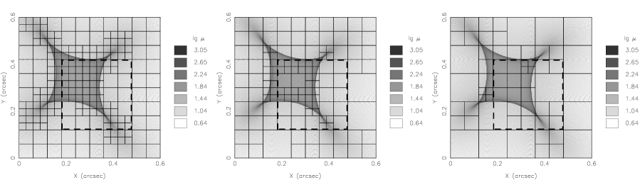
Figure 1: Source plane pixelisations corresponding to splitting factors of $s=$4, 9, and 14 from left to right. The grey scale shows log(magnification) calculated from the best fit dual–component lens model in Section 4.1. Heavy dashed box shows the $0.3^{\prime\prime}\times 0.3^{\prime\prime}$ source plane size used in the reconstruction throughout this paper.

We determine an optimal value of $s$ empirically, by measuring the improvement in the fit brought about by the splitting for different values of $s$, successively reducing the value of $s$ to the point at which no significant improvement is obtained. In detail, starting with a large value of $s$, the source plane is pixelised as described, and the best fit model is recomputed (see Section 3.3). This gives a set of minimised lens model parameters, the reconstructed source surface brightness distribution and the value of $\chi^{2}$ for the fit. The value of $s$ is then reduced, the procedure repeated, and the new value of $\chi^{2}$ computed. If the reduced value of $s$ increases the number of source pixels by $\Delta I$, then this is the decrease in the number of degrees of freedom. The change $\Delta\chi^{2}$ should therefore be distributed as $\chi^{2}$ for $\Delta I$ degrees of freedom, since we have simply increased the number of linear parameters in the fit. If $\Delta\chi^{2}$ is significant by this test, the lower splitting factor is accepted and the next lower value of $s$ is then tested. We set the significance level at the conservative value of $1\%$, for the reasons given above.

Figure 1 illustrates the changing pixelisation as the splitting factor is decreased successively through the values, 14, 9, 4, from right to left. In each plot, the grey scale is the $\mu$ map. We find that the middle value $s=9$ corresponds to the $1\%$ significance level chosen, for all three lens models described in Section 3.2. Comparison of the goodness of fit of each model in Section 4.1 is therefore carried out with an adaptive source grid constructed using $s=9$.

In order to ensure a completely fair comparison between models, a further effect must be taken into consideration. The chosen offset of the source plane centre with respect to the centre of the lens caustic structure can in principle bias the goodness of fit of one lens model relative to another. Each of the three lens models tested has a slightly different caustic shape. A given source plane offset can result in a more effective adaptive pixel grid for one lens model than another due to fortuitous alignment of pixel edges relative to the lens caustic. We deal with this effect, essentially, by including the source plane offset in the minimisation; we perform a full lens $+$ source minimisation at every point on a regular grid of offsets and take the best overall fit. This is discussed further in Section 3.3.

Our method of adaptively pixelising the source plane in this way solves the problem noted by Kochanek, Schneider & Wambsganss (2004) that plagues current pixelised source based methods. Existing techniques use a regular source grid and thereby rely on some form of regularisation to control the behaviour of the reconstructed source in regions of low magnification. Regularisation smooths the source light profile, reducing the effective total number of parameters and hence increasing the number of degrees of freedom, by an amount that cannot be quantified. This is especially problematic when comparing different lens models, as a fixed regularisation weight for one model generally would not give the same increase in number of degrees of freedom for another. In our scheme, the splitting factor has been chosen such that the adaptively sized pixels extract maximum information from the lens image without need of regularisation. Therefore, the number of degrees of freedom of the fit is a well–defined number. This allows, firstly, unambiguous assessment of whether a given model provides a satisfactory fit to the data and secondly, unbiased comparison of different model fits.

3 Data and method of analysis

In this section we provide details of the observational data (3.1) and the lens models considered (3.2). We also discuss the practicalities of performing the minimisation (3.3) and explain the calculation of the uncertainties (3.4).

3.1 HST observations

The data analysed here are the same data analysed by Wayth et al. (2004), who give full details of the observations and data reduction. In order to keep the current paper self–contained, the key elements are outlined in this section.

The field of 0047$-$2808 was observed with HST’s WFPC2 instrument in the F555W filter over four orbits. We used the WFC, which has $0.1\arcsec$ pixels. The chosen filter ensured that the strong Ly$\alpha$ emission from the source star–forming galaxy at $z=3.595$ (Warren et al., 1996) was detected, thereby enhancing the ring:lens flux ratio. Observations were dithered using a $2\times 2$ pattern with a horizontal and vertical step size equal to $N+0.5$ pixels. At each of the four dither positions, two exposures of 1200s were taken to aid cosmic ray removal.

After subtracting the background counts from each exposure and eliminating cosmic rays, pairs of exposures at each dither position were averaged. These four combined images were then used to form an interlaced image with pixel interval $0.05^{\prime\prime}$. This image is reproduced in Figure 2. In the figure the pixels are shown with side $0.05^{\prime\prime}$, but this is only for presentational purposes. In the analysis, we account for the true size of $0.1^{\prime\prime}$ by fitting simultaneously to the four images that make up the interlaced image.

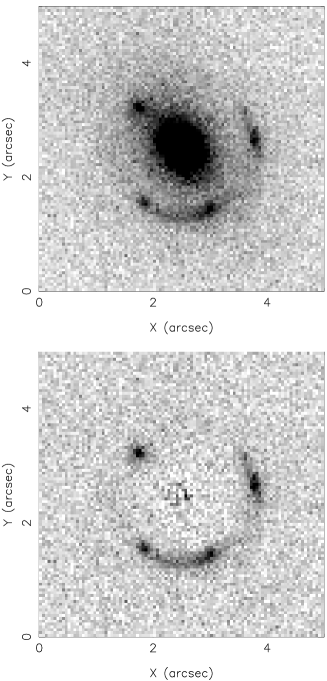
Figure 2: Top: Interlaced HST image of $0047-2808$ with pixel interval $0.05^{\prime\prime}$. Bottom: Interlaced image after subtracting the image of the lensing galaxy. In this figure, the position angle of the vertical axis is $27.44^{\circ}$ E of N.

We constructed a noise frame for this image for the purposes of measuring $\chi^{2}$, both for fitting the light profile of the lensing galaxy and for the lensing analysis. Our Poisson estimate of the pixel flux uncertainties allows for photon noise and readout noise, and accounts for the removal of cosmic rays.

The image of the lensing galaxy was subtracted by fitting a Sérsic profile (Sérsic, 1968) plus a central point source (Wayth et al., 2004). The best fit was found by minimising $\chi^{2}$, discounting an annular area containing the image of the lensed source. In the fitting procedure profiles were convolved with a model WFPC2 psf and the appropriate pixel scattering kernel. The lower half of Figure 2 shows the resulting Einstein ring after the lensing galaxy has been subtracted. The residue at the centre of the subtracted image is not significant, given the high counts at the centre of the lens galaxy image. This is the image used in the lensing analysis.

3.2 Lens models

Wayth et al. (2004) used the same data analysed in the current paper to test a range of commonly used lens mass models. Three models failed to provide a satisfactory fit. These were: 1) a model in which the mass profile follows the light profile, with a single free parameter, $M/L$, 2) the NFW model $\rho(r)=\frac{\rho_{s}}{(r/r_{s})(1+r/r_{s})^{2}}$ (Navarro, Frenk & White, 1996), with $r_{s}=25$kpc, a value suggested by N–body simulations for galaxies of this mass, 3) a model of a singular isothermal sphere with external shear. In contrast, the singular isothermal ellipsoid (SIE) model, as well as three other similar models, were found to provide satisfactory fits. Nevertheless, a general power–law model, of which the SIE is a special case, gave a better fit than the SIE model, at a marginally significant level.

The current paper follows on from Wayth et al. (2004). Since the formalism of the semi–linear method is different from the maximum–entropy method applied by Wayth et al. (2004) (Section 1), we repeat part of their analysis by fitting the SIE and power–law models, confirming their conclusion that the power–law model is preferred. We then go on to test a dual–component model, comprising baryons and dark matter. Details of the various models are provided below.

We use coordinates $x,y$ defined by the axes of the CCD array and centred on the centre of the galaxy light distribution. The models include mass components with elliptical surface mass densities characterised by four parameters; the coordinates of the centre $x,y$, the axis ratio $q=b/a$ (i.e. the ratio of the semi–minor axis to the semi-major axis), and the orientation of the semi–major axis $\theta$, defined as the angle measured counter–clockwise from the vertical. The surface mass density profiles are parameterised in terms of the ellipse coordinate $\xi$, defined by $\xi^{2}=x^{\prime 2}+y^{\prime 2}/q^{2}$, where $x^{\prime}$, and $y^{\prime}$, are coordinate axes aligned with the semi–major and semi–minor axes of the ellipse.

For each mass model the components of the deflection angle vector $\alpha$ are computed from the surface mass density profile $\Sigma(\xi)$ using the method of Schramm (1990), as parameterised by Keeton (2001);

$$(\alpha_{1},\alpha_{2})=(qx^{\prime}J_{0}(x^{\prime},y^{\prime}),qy^{\prime}J_{1}(x^{\prime},y^{\prime}))$$ (7)

where

$$J_{n}(x^{\prime},y^{\prime})=\int^{1}_{0}\frac{\Sigma(\xi)/\Sigma_{c}}{[1-(1-q^{2})u]^{n+1/2}}{\rm d}u$$ (8)

and where $\Sigma_{c}$ is the critical surface mass density and

$$\xi(u)^{2}=u\left(x^{\prime 2}+\frac{y^{\prime 2}}{1-(1-q^{2})u}\right).$$ (9)

The different models are tested against each other by comparing the best fit values of $\chi^{2}$ in relation to the numbers of degrees of freedom of the models. In all cases we eschew regularisation and use the formalism previously described to select the optimal pixelisation of the source plane so that the number of degrees of freedom is well defined.

3.2.1 SIE and singular power–law models

The power–law model has a volume mass density profile of the form

$$\rho(r)=\rho_{0}(r/r_{0})^{-\alpha}$$ (10)

where $r_{0}$ is arbitrarily chosen. We allow the coordinates of the centre of the mass to be offset from the centre of the light. Adding $\rho_{0}$ and $\alpha$ to the four parameters of the ellipse, the power–law model has 6 parameters. The SIE model is the special case $\alpha=2$, and has 5 parameters.

3.2.2 Baryons + dark matter halo model

We assume that the projected surface mass density of the baryonic component of the lens model follows the surface brightness distribution of the lens galaxy. The baryons are therefore fixed in shape as determined by the Sérsic $+$ point source profile fitted to the image. In our analysis, the baryonic contribution to the total mass profile is determined by the rest–frame B–band baryonic $M/L$, $\Psi$ (in units $h_{65}M_{\odot}/L_{B\odot}$), which is left as a free parameter in the minimisation. (In converting from the F555W filter to the rest–frame B–band, we have adopted the $k-$correction and the band zero–point difference computed by Koopmans & Treu (2003) (see Wayth et al. (2004) for details).) The lens deflection angle due to the baryons is hence calculated from the elliptical surface mass density of the fitted Sérsic profile which, in units of $M_{\odot}/\Box^{\prime\prime}$, is

$$\Sigma_{b}(\xi_{b})=\Psi L_{1/2}\exp\{-5.90[(\xi_{b}/1.09^{\prime\prime})^{0.32}-1]\}$$ (11)

and the mass of the central point source,

$$M_{p}=3.09\times 10^{9}\,h_{65}^{-2}\,L_{B\odot}\Psi,$$ (12)

expressed here in units of $M_{\odot}$. The fitted half light luminosity of the Sérsic profile is $L_{1/2}=(1.99\pm 0.09)\times 10^{9}h_{65}^{-2}L_{B\odot}/\Box^{\prime\prime}$. The axis ratio measured from the light distribution is $q_{b}=0.69$ (Wayth et al., 2004). Since the 4 parameters of the ellipse are the measured values for the Sérsic fit, the baryonic component of the mass model has a single free parameter $\Psi$. Note that the deflection angles for this model need only be computed once, and then scaled by $\Psi$ as $\Psi$ is varied in searching for the best–fit mass model.

For the dark matter halo, we choose a generalised NFW model (Navarro, Frenk & White, 1996) which allows for a variable central density profile slope $\gamma$. This has a volume mass density profile given by

$$\rho(r)=\frac{\rho_{s}}{(r/r_{s})^{\gamma}(1+r/r_{s})^{3-\gamma}}.$$ (13)

Here, $\rho_{s}$ is the halo normalisation and $r_{s}$ is a scale radius. To convert this to a projected surface mass density profile, we integrate along the line of sight following the prescription of Keeton (2001). This integration, which must be evaluated numerically, gives a radially symmetric surface mass density profile. As with the Sérsic profile, ellipticity is introduced by replacing the radial coordinate with an ellipse coordinate $\xi_{h}$ that has an associated axis ratio $q_{h}$.

In total there are 6 free parameters for the dark–matter mass profile, $x_{h},y_{h},q_{h},\theta_{h},\rho_{s},\gamma$. We hold the scale radius fixed at $r_{s}=50h_{65}^{-1}$kpc $(\cong 8^{\prime\prime}\,\,@\,z=0.485)$ to match that expected from simulations by Bullock et al. (2001) for a galaxy of similar mass and redshift as the lens galaxy in $0047-2808$. In Section 3.4 we discuss the effect of changing $r_{s}$, although since it is much larger than the radius of the ring traced by the observed images $r=1.16^{\prime\prime}$, this effect is small.

The overall deflection angle at any point in the lens plane resulting from the combined effect of the baryonic and halo mass is simply given by the addition of the separate deflection angles due to the point mass, the Sérsic profile and the generalised NFW halo.

The combined model, baryons and dark matter, has 7 parameters.

3.3 Minimisation procedure

A full minimisation for a given lens model involves three nested processes. The innermost process is the linear inversion step explained in Section 2, giving a reconstructed source and $\chi^{2}$ from equation (1) for a trial set of lens model parameters. The middle process minimises the lens model parameters and for this we use Powell’s method (Press et al., 2001). Finally, at the outermost level, we step through a grid of source plane offsets to address the effect discussed in Section 2.1, that fortuitous alignments of the source pixel grid with the lens caustic can bias the fit. We step through a $10\times 10$ grid of offsets of size $0.006^{\prime\prime}$, corresponding to a tenth of a medium-sized pixel in Figure 1. The best overall fit is taken as the lowest value of $\chi^{2}-N_{dof}$.

In computing the images of each source pixel, we sub-grid each image plane pixel into a $4\times 4$ array of sub–pixels. Rays are traced back from the image plane to the source plane via each image plane sub–pixel. The sub–gridding was chosen to ensure a smooth $\chi^{2}$ surface, necessary for reliable minimisation.

For the dual–component model we calculate joint confidence regions in the $\gamma-\Psi$ plane by marginalising over the remaining 5 parameters, at regular grid points spanning this plane. At every point in the $\gamma-\Psi$ plane, the minimisation is initialised with the halo centred on the Sérsic centre and possessing the same orientation and ellipticity as the visible light. The normalisation of the halo must be initialised by a fitted function as explained below. Satisfactory convergence is reliably obtained by setting an arbitrarily small tolerance and terminating minimisation once 200 iterations have been performed.

We find at all points in the parameter space that the variation of $\chi^{2}$ with halo normalisation has three minima near the correct lens solution. One is the correct solution, defined such that the reconstructed source surface–brightness distribution is most compact. In addition there are two local minima corresponding to under and over magnifications. In the under magnified case, the reconstructed source surface brightness distribution is a smaller, slightly distorted version of the observed ring image. In the over magnified case, the source resembles a small ring image but inverted such that every pixel in the ring has been reflected in a plane running through the ring centre and perpendicular to the pixel’s radial vector. Both under and over magnified source reconstructions can be rejected on the grounds that they produce extraneous images when lensed to the image plane. To prevent convergence to an incorrect local minimum, we initialise the halo normalisation $\rho_{s}$ to a value which is estimated to lie close to the correct solution. This initial value is set by a fitting function derived from a simplified analysis in which only $\rho_{s}$ is allowed to vary across the $\gamma-\Psi$ plane.

3.4 Modelling uncertainty

The uncertainty on the set of reconstructed lens model parameters is determined from the prescription in WD03. This is calculated by inverting the curvature matrix for all parameters, including the source pixels, to obtain the full covariance matrix. The uncertainty from the fit for a given parameter is then just the relevant diagonal term in this matrix. For the dual–component model, we determine the error on $\gamma$ and $\Psi$ directly from their marginalised $\chi^{2}$ contours. The total error that we quote for $\Psi$ includes an extra contribution from the only source of significant uncertainty in the Sersic profile; the parameter $L_{1/2}$ (see 3.2.2).

A final source of error in our dual–component model stems directly from the uncertainty on the scale radius $r_{s}$ in the halo component. Dalal & Keeton (2003) argue that $r_{s}$ should be left as a free parameter in the minimisation. We have opted to hold $r_{s}$ at the value of $50h_{65}^{-1}$kpc as expected from simulations by Bullock et al. (2001) and search for a solution in the context of this model. Our data can only weakly constrain $r_{s}$ which has the advantage that our results do not depend sensitively on its value. We find that a 10% change in $r_{s}$ produces a $\sim 1\%$ change in the minimised $M/L$ and a negligible change in $\gamma$. This error is not included in the final error budget.

4 Results

This section is divided into two halves. In the first, Section 4.1, the three lens models are compared. In the second, Section 4.2, the dual–component model is considered in more detail and using this model, we reconstruct the source surface brightness distribution.

4.1 Comparison of Models

In this section, we compare the performance of the three models, 1. SIE, 2. power-law, and 3. dual–component models, in fitting the observed ring image. We also compare our findings with the analysis by Koopmans & Treu (2003) who analysed 0047$-$2808 using a method combining dynamical measurements and lensing.

All reconstructions in this section are unregularised. As explained in section 2.1 this is to allow unbiased comparison of models. The $\chi^{2}$ is evaluated in an annular masked region shown in the bottom left panel of Figure 5. The mask was designed to ensure that it includes the image of the entire source plane, with minimal extraneous sky. This means that only significant image pixels are used in the fit, making $\chi^{2}$ more sensitive to the model parameters.

Table 1 summarises the results, listing the best–fit value of $\chi^{2}$ and the number of degrees of freedom (NDF) of that fit. Recall that the NDF depends not only on the number of parameters of the mass model, but also on the exact source pixelisation used, which in turns depends on the structure of the caustics.

Model	$\chi^{2}_{min}$	NDF
SIE	1156.2	1247
power–law	1157.7	1255
baryons+halo	1161.4	1269

Table 1: Performance of singular isothermal ellipsoid (SIE), power–law, and dual–component models, in terms of minimum $\chi^{2}$ and number of degrees of freedom.

Parameter	Minimised Value	$1\sigma$ error in fit
$\rho_{s}$	$3.27\times 10^{6}$	$0.22\times 10^{6}$
$(x_{h},y_{h})$	$(0.070^{\prime\prime},0.026^{\prime\prime})$	$(0.004^{\prime\prime},0.005^{\prime\prime})$
$q_{h}$	0.820	0.020
$\theta_{h}$	$41.7^{\circ}$	$1.5^{\circ}$

Table 2: Remaining minimised parameters for halo in the dual–component model. Reading from top to bottom, parameters are; normalisation in units of $h^{2}_{65}M_{\odot}$kpc^-3, offset from light centre, axis ratio, and orientation of semi–major axis from vertical in counter–clockwise direction. The $1\sigma$ error is derived from the full covariance matrix.

4.1.1 SIE and power–law models

For the SIE model, $\alpha=2$, the best fit gives $\chi^{2}_{min}=1156.2$ for 1247 degrees of freedom. The power–law model gives $\chi^{2}_{min}=1157.7$ with 1255 degrees of freedom, and a measured slope $\alpha=2.11\pm 0.04$. The increase in the NDF is because fewer pixels are used to tessellate the source plane. Comparing the power–law to the SIE model, the increase in $\chi^{2}$ of $\Delta\chi^{2}=1.5$, only, for an increase of 8 degrees of freedom differs from the expectation of $\Delta\chi^{2}\sim 8$ at a significance level of $99.3\%$. The power–law model therefore is a significant improvement over the SIE model. This is reflected in the measured value of $\alpha=2.11$ which is inconsistent with $\alpha=2$ at the $2.7\sigma$ significance level.

Wayth et al. (2004) compared the same two models, using a maximum–entropy inversion method. This method entails regularisation of the inversion. They applied minimal regularisation (such that the inversion amounts to the non–negative min–$\chi^{2}$ solution), in order to minimise the uncertainty in the change in the NDF. They found that the power-law model gives a better fit than the SIE, at an associated significance level of $96\%$. They found $\alpha=2.08\pm 0.03$ for the power-law model as well as orientations and ellipticities for both models consistent with our findings. These results are in good agreement with ours, vindicating their approach for dealing with the problem of the uncertainty of the NDF.

4.1.2 Baryons + dark matter halo model

With the dual–component model, we obtain $\chi^{2}_{min}=1161.4$ for 1269 degrees of freedom. Comparing this against the best fitting singular power–law model gives an increase in $\chi^{2}$ of $\Delta\chi^{2}=3.7$, only, for an increase of 14 degrees of freedom. This small increase in $\chi^{2}$, differs from the expectation of $\Delta\chi^{2}\sim 14$ at a significance level of $99.7\%$, demonstrating that the dual–component model provides a significantly better fit.

Figure 3 shows the $\chi^{2}$ contours in the $\gamma-\Psi$ plane, marginalised over the remaining 5 parameters. The grey shaded regions give the 68%, 95%, 99% & 99.9% one–parameter confidence limits. We obtain an inner slope of $\gamma=0.87^{+0.69}_{-0.61}$ to 95% confidence (or a limit of $\gamma<1.74$ to $99.9\%$ confidence) and a $M/L$ of $\Psi=3.05^{+0.53}_{-0.90}\,h_{65}\,M_{\odot}/L_{B\odot}$ to 95% confidence, including the photometric error (or $\Psi=3.05^{+0.78}_{-1.30}\,h_{65}\,M_{\odot}/L_{B\odot}$ to $99.9\%$ confidence). The remaining five minimised lens model parameters are provided in Table 2.

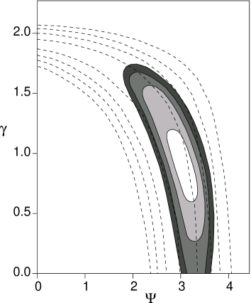
Figure 3: One–parameter confidence regions on inner slope and baryonic $M/L$: 68%, 95%, 99% & 99.9%. Dashed lines are same confidence regions from analysis by Koopmans & Treu (2003).

The dashed lines in Figure 3 show the same confidence levels obtained by Koopmans & Treu (2003) in analysis of the same HST data as in this paper. Their result used the total mass enclosed by the Einstein ring and in addition, the measured velocity dispersion profile of the lens galaxy, as constraints. Clearly, our semi–linear method, in using all the information contained within the ring image, significantly reduces the uncertainty in the lens model. Overall the two results are in very good agreement, bearing in mind that our result comes from a purely gravitational lens analysis, while theirs is primarily a dynamical analysis, supplemented by the size of the Einstein ring.

With reference to the other minimised parameters given in Table 2, we conclude that; 1) the centre of the baryons is closely aligned with the halo centre, 2) the halo, with $q_{h}=0.82\pm 0.02$, is significantly rounder than the stellar component of the galaxy, with $q_{b}=0.69\pm 0.01$, 3) there is a significant difference between the baryonic orientation of $\theta_{b}=35.0\pm 0.7$ and that of the halo $\theta_{b}=41.7\pm 1.5$ .

4.2 Further Analysis

In the previous section we established that the baryon+dark matter halo model provides a significantly better fit to the observed ring compared to single component models. We now analyse this model in more detail.

4.2.1 Baryonic mass & light

As Figure 3 shows, we have been able to constrain the baryonic $M/L$ without the need for dynamical measurements. This is the first time a pure lensing analysis of a single system has measured the baryonic $M/L$ directly. Being a lens estimated quantity, this is free of the uncertainties associated with dynamical methods (see Section 1).

Koopmans & Treu (2003) show that the lens galaxy in 0047$-$2808 is offset from the local fundamental plane by a factor 0.37dex. This value is in close agreement with the expected passive evolution of this galaxy, estimated from population synthesis models matched to the measured $V-I$ colour (Wayth et al., 2004). Correcting by this factor, our derived $M/L$ $\Psi=7.1$ is remarkably similar to the local average value for the centres of ellipticals of $7.3\pm 2.1\,h_{65}\,M_{\odot}/L_{B\odot}$ (Gerhard et al., 2001; Treu & Koopmans, 2002), determined dynamically. Either this is a coincidence, or it is an indication that the various elements going into this comparison, i.e. our lensing analysis, the local dynamical analysis, the population synthesis models, and the assumption of passive evolution, are all quite accurate.

4.2.2 Halo and baryonic fractions

We calculate the fractional contribution of the baryons to the total projected mass by integrating the projected mass distribution of each component inside a circular aperture of radius $1.16^{\prime\prime}$ placed at the lens centre (the offset between components is small enough to disregard). Within this aperture, the baryons account for $65^{+10}_{-18}$% (95% CL) of the total projected mass.

The fraction of dark matter inside a sphere of the same radius is obtained by deprojecting both surface mass density profiles. Because lensing measures only projected mass, we have no information regarding its distribution along the line of sight and so this must be assumed. Our approach is to first calculate a circularly averaged surface density profile for each component and then deproject assuming spherical symmetry. Deprojection is carried out using the approach given by Binney & Tremaine (1987).

We find that the baryons account for $84^{+12}_{-24}$% (95% CL) of the total mass within a sphere of radius $1.16^{\prime\prime}(7.5h_{65}^{-1}$kpc). Figure 4 plots both the circularly averaged surface mass density profile and the cumulative deprojected mass profile for the halo and baryons. In the case of the baryons, the point mass is included.

Figure 4: Circularly averaged projected surface mass density profile of halo (solid) & baryons (dashed), and cumulative 3–dimensional mass profile of halo (dot–dash) and baryons (dotted). Vertical dashed line is mean radius $1.16^{\prime\prime}$ of the ring traced by the lensed images.

4.2.3 Source reconstruction

The reconstructed source and image for the best-fit dual component model are shown in Figure 5. The top row of this figure shows the unregularised result. Note the correspondence between the pixelisation in these three panels, and that in the middle panel of Figure 1. The top–left panel (side $0.3\arcsec$) shows the reconstructed source, and the bottom middle panel (side $4.2\arcsec$) is the image of this source, convolved with the WFC psf. This is the best–fit to the actual image shown in the bottom left–hand panel. The uncertainties on the source pixel surface brightnesses are shown in the top middle panel, and the corresponding significance map (ie. surface brightness divided by standard errors) is shown in the top right–hand panel. Note that, in contrast with similar maps shown in WD03, where the uncertainties were noticeably smaller inside the caustic, here they are more uniform across the source plane, as a consequence of the pixel size varying with the magnification.

The limited source plane resolution allowed for these data by our adaptive pixelisation scheme is a consequence of the relatively large WFC pixels, and the relatively low S/N of the image. Nevertheless there are clearly two areas in the source plane, of high significance, where the source flux is concentrated, one on either side of the caustic. This is the same conclusion reached by Wayth et al. (2004). A better sampled image of high S/N would allow formation of a clearer picture of the nature of the source galaxy. Obviously, the source light profile does not follow a simple parametric form. This means that attempting to model 0047$-$2808 by forming model images using a simple single source would bias the fitted model parameters.

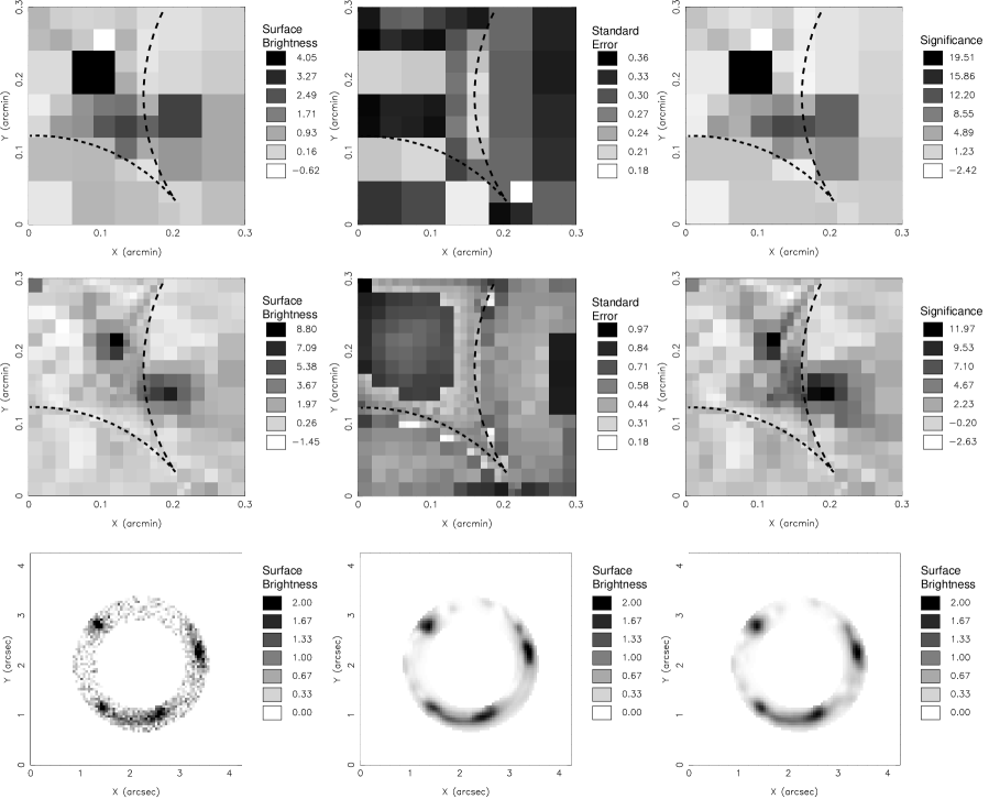
Figure 5: Reconstructed source from best fit lens model (caustic shown by dashed heavy line). Top left: Unregularised reconstructed source surface brightness distribution obtained in Section 4.2.3. Top middle: Standard errors on unregularised source pixels. Top right: Significance of unregularised source. Middle left: Regularised source from best fit lens model. Middle: Standard errors on regularised source. Middle right: Significance of regularised source. Bottom left: Masked observed ring image. Bottom middle: Lensed image of unregularised source. Bottom right: Lensed image of regularised source

Purely for the purposes of visualisation, we also performed a regularised inversion. The results are provided in the middle row of Figure 5. For this, the regularisation weight, $\lambda$, was chosen to make $\chi^{2}$ and the regularisation term in equation (4) contribute equally to the figure of merit $G$. Setting the minimum allowed source pixel size to $0.01^{\prime\prime}\times 0.01^{\prime\prime}$, we followed the same procedure, set out in Section 2.1, to select the splitting factor. The clarity of the source is somewhat improved. The outer source appears to be extended, and to straddle the caustic. The significance plot, right–hand panel, middle row, identifies both source components as being highly significant. The reconstructed image, bottom right–hand panel, is somewhat smoother, as expected.

5 Discussion and summary

One of the main goals of this paper was to investigate the extent to which a pure gravitational lens analysis of the image of an extended source, using all the information in the image, could constrain the inner slope of the dark matter density distribution in the lens galaxy. Applying the method to the lens $0047-2808$, we have succeeded in shrinking the uncertainties considerably, compared to the lens+dynamical analysis of Koopmans & Treu (2003), which used only the positions of the four brightest peaks in the image as lens constraints. Our measurement of the inner slope of the dark matter halo of $\gamma=0.87^{+0.69}_{-0.61}$ (95% CL) is consistent with the cuspy prediction of the CDM model. Nevertheless, we find that the dark matter makes only a minor contribution to the total mass within a spherical radius equal to the Einstein radius of the lens. There is mounting evidence from both dynamical and lensing methods that this is fairly typical of bright and intermediate–luminosity early–type galaxies. For example, Romanowsky et al. (2003) compared the measured motions of planetary nebulae around three nearby ellipticals, out to several effective radii, with dynamical models without dark matter and found satisfactory agreement. A similar, more quantitative, conclusion was reached by a statistical analysis of 22 multiply–imaged quasars, by Rusin, Kochanek & Keeton (2003). Although a single multiply–imaged quasar is not useful for constraining dual–component models, by assuming a fixed ratio of dark matter to baryons (within two effective radii), the same power–law slope $\gamma$ for the dark matter in all systems, and by invoking a relation between $\Psi$ and galaxy luminosity, Rusin, Kochanek & Keeton (2003) were able to derive useful constraints on dual–component models. By fixing the inner slope to the NFW value $\gamma=1$, they find that the baryons account for $78\%\pm 10$ of the projected total mass within two effective radii, average $7h_{65}^{-1}$kpc. This is consistent with our measurement of $65\%^{+10}_{-18}(95\%CL)$, within $7.5h_{65}^{-1}$kpc, again in 2D. Note that we are able to achieve similar constraints from a single system, with fewer assumptions. This highlights the usefulness of images of extended sources.

As Figure 4 shows, the baryons are more concentrated than the dark matter in this lens galaxy, and dominate the mass distribution within the region of the image. The baryons will alter the shape of the dark matter halo, predicted by the pure dark matter simulations, in a non–trivial way, dependent on the history of assembly of the various components, the sequence of star formation, and the extent to which gas is blown out of the galaxy by winds. A simple treatment for estimating the influence of baryons is the so called ‘adiabatic approximation’ of Blumenthal et al. (1986). In this approximation, the expected profile of a collapsed halo can be estimated from its initial profile and the initial and collapsed baryonic profiles, assuming the halo adiabatically contracts. By applying this in reverse, the initial halo profile can be estimated from the collapsed profile as determined from a two component model such as ours. This initial profile can then be compared directly with the pure dark matter CDM simulations. Treu & Koopmans (2002) used this reverse method on their two component model of the lens system MG2016$+$112. They found that the inner slope of the initial halo can be substantially shallower than the measured collapsed slope. If this is a valid approximation, then a similar effect would be expected for 0047$-$2808. This result is of interest for the case where the measured slope $\gamma$ is already significantly smaller than the predicted value, $\gamma\sim 1$, since it acts to widen the discrepancy. But given the simplifications involved, and therefore the uncertainty in the magnitude of the effect, it is of limited interest in the present case where our best–fit value is consistent with the CDM value.

For our dual component model we found that the dark halo is offset in orientation from the baryons by $6.7^{\circ}\pm 1.7$, and is rounder, with a significant difference in axis ratio of $\Delta q=0.13\pm 0.02$. Our model is a simple one, given the relatively low S/N of the image, and does not include external shear. Nevertheless, the galaxy does not lie in a dense environment, as evidenced by the image provided in Warren et al. (1999). There would be some degeneracy in a solution including shear, between the amount of shear and the orientation offset (see Keeton et al. (1997) for a discussion). A deeper image, with smaller pixels, would justify a more sophisticated analysis. To gauge the potential improvement, we have undertaken extensive simulations of observations of 0047$-$2808 with the HST Advanced Camera for Surveys. Using the High Resolution Channel over 10 orbits, with application of the semi–linear method we anticipate a reduction in the error on $\gamma$ by a factor of $\sim 5$, sufficient to strongly test the CDM expectation. The improvement is a consequence of the high throughput of ACS, and especially the smaller pixel size.

We conclude with a summary of the main points of the paper:

1. We have extended the semi–linear method of WD03 for inverting gravitational lens images of extended sources, to include adaptive pixelisation of the source plane. We have identified a method for tessellating the source plane that applies an objective criterion for sub–dividing pixels, which maximises the information about the source extracted from the image, and is also stable. Because of this the inversion does not require regularisation. This eliminates the problem that with regularised inversion the number of degrees of freedom is ill defined. Proper statistical comparison of different mass models is thereby enabled.

2. We have applied our semi–linear method to HST-WFPC2 observations of the Einstein ring system 0047$-$2808 to determine the lens galaxy mass profile. We confirm the result of Wayth et al. (2004) that a power–law model, $\alpha=2.11\pm 0.04$ produces a significantly better fit than the single isothermal ellipsoid model. Furthermore our analysis shows that a dual–component model, comprising a baryonic Sérsic profile + point mass nested in a dark matter generalised NFW halo, gives a significantly better fit ($3.0\sigma$) to the data than the best power–law model. We demonstrated that using 100% of the information contained in the Einstein ring image, with an adaptive source plane pixel scale, provides significantly better constraints than the modelling of Koopmans & Treu (2003), who used the measured radial variation of the stellar velocity dispersion, plus the lens constraints provided by the positions of the four brightest peaks in the ring.

3. For the dual–component model, we find that the baryonic component has an unevolved rest–frame B–band $M/L$ of $3.05^{+0.53}_{-0.90}\,h_{65}\,M_{\odot}/L_{B\odot}$. This $M/L$ was obtained without any dynamical measurements and is therefore not subject to the usual uncertainties associated with this approach. The errors quoted here include the photometric uncertainty. Evolving this value to zero redshift gives a result consistent with the dynamically–measured $M/L$ in the centres of nearby ellipticals.

4. The measured inner slope of the dark–matter halo is $\gamma=0.87^{+0.69}_{-0.61}$ (95% CL), consistent with the predictions of CDM simulations.

5. We find that the baryons account for $65^{+10}_{-18}$% (95% CL) of the total projected mass or, assuming spherical symmetry, $84^{+12}_{-24}$% (95% CL) of the total deprojected mass within a radius of 1.16” ($7.5h_{65}^{-1}$kpc) traced by the ring.

6. We find that the dark–matter halo is significantly misaligned with the stellar light, and also is significantly rounder.

7. The reconstructed source surface brightness distribution shows two distinct source objects in agreement with the findings of Wayth et al. (2004). This highlights the need for non–parametric sources to obtain unbiased lens mass profiles.

Acknowledgements

We would like to thank Paul Hewett, Geraint Lewis, Leon Lucy, and Randall Wayth for helpful discussions. SD is supported by PPARC.

References

- Binney (2004) Binney, J., 2004, in ’Dark Matter in Galaxies’, IAU Symposium 220, ed. Stuart Ryder, D.J. Pisano, Mark Walker & Ken Freeman, Publ. Astron. Soc. Pac
- Binney & Tremaine (1987) Binney, J. & Tremaine, S., 1987, ’Galactic Dynamics’, Princeton University Press
- Biretta et al. (2002) Biretta, J., Lubin, L., et al., 2002, HST WFPC2 Instrument Handbook Version 7.0, Baltimore, STScI
- Blumenthal et al. (1986) Blumenthal, G.R., Faber, S.M, Flores, R., Primack, J.R., 1986, ApJ, 301, 27
- Bullock et al. (2001) Bullock, J.S., Kollat, T.S., Sigad, Y., Somerville, R.S., Kravtsov, A.V., Klypin, A.A., Primack, J.R., Deckel, A., 2001, MNRAS, 321, 598
- Dalal & Keeton (2003) Dalal, N. & Keeton, C.R., 2003, astro-ph/0312072
- de Blok et al. (2001) de Blok, W.J.G., McGaugh, S.S., Bosma, A., Rubin, V.C., 2001, ApJ, 552, 23
- de Blok & McGaugh (1997) de Blok, W.J.G. & McGaugh, S.S., 1997, MNRAS, 290, 533
- Gerhard et al. (2001) Gerhard, O., Kronawitter, A., Saglia, R.P., & Bender, R., 2001, AJ, 121, 1936
- Hayashi et al. (2003) Hayashi, E., Navarro, J.F., Power, C., Jenkins, A., Frenk, C.S., White, S.D.M., Springel, V., Stadel, J., Quinn, T., 2003, submitted to MNRAS, astro-ph/0310576
- Keeton (2001) Keeton, C.R., 2001, astro-ph/0102341
- Keeton et al. (1997) Keeton, C.R., Kochanek, C.S., Seljak, U., 1997, ApJ, 482, 604
- Kochanek, Schneider & Wambsganss (2004) Kochanek, C.S., Schneider, P., Wambsganss, J., 2004, Part 2 of Gravitational Lensing: Strong, Weak & Micro, Proceedings of the 33rd Saas-Fee Advanced Course, G. Meylan, P. Jetzer & P. North, eds. (Springer-Verlag: Berlin)
- Koopmans & Treu (2003) Koopmans, L.V.E. & Treu, T., 2003, ApJ, 583, 606
- Krist (1995) Krist, J. E., 1995, ”WFPC2 Ghosts, Scatter, and PSF Field Dependence,” in Calibrating Hubble Space Telescope: Post Servicing Mission, eds. A. Koratkar and C. Leitherer, p. 311
- Moore et al. (1998) Moore, B., Governato, F., Quinn, T., Stadel, J., Lake, G., 1998, ApJ, 499, L5
- Moore et al. (1999) Moore, B., Quinn, T., Governato, F., Stadel, J., Lake, G., 1999, MNRAS, 310, 1147
- Navarro et al. (2004) Navarro, J.F., Hayashi, E., Power, C., Jenkins, A., Frenk, C.S., White, S.D.M., Springel, V., Stadel, J., Quinn, T.R., 2004, MNRAS, 349, 1039
- Navarro, Frenk & White (1996) Navarro, J.F., Frenk, C.S. & White S.D.M., 1996, ApJ, 462, 563
- Power et al. (2003) Power, C., Navarro, J.F., Jenkins, A., Frenk, C.S., White, S.D.M., Springel, V., Stadel, J., Quinn, T., 2003, MNRAS, 338, 14
- Press et al. (2001) Press, W.H., Teukolsky, S.A., Vetterling, W.T., Flannery, B.P., 2001, ’Numerical Recipes in Fortran 77, 2nd Edition’, Cambridge University Press
- Romanowsky et al. (2003) Romanowsky, A.J., Douglas, N.G., Arnaboldi, M., Kuijken, K., Merrifield, M.R., Napolitano, N.R., Capaccioli, M., Freeman, K.C., 2004, Science, 301, 1696
- Rusin, Kochanek & Keeton (2003) Rusin, D., Kochanek, C.S., & Keeton C.R., 2003, ApJ, 595, 29
- Sand, Treu & Ellis (2002) Sand, D.J., Treu, T., & Ellis, R.S., 2002, ApJ, 574, L129
- Sand et al. (2004) Sand, D.J., Treu, T., Smith, G.P., Ellis, R.S., 2004, ApJ, 604, 88
- Schramm (1990) Schramm, T., 1990, A&A, 231, 19
- Sérsic (1968) Sérsic, J.L., 1968, Cordoba, Argentina: Observatorio Astronomico (1968)
- Spergel & Steinhardt (2000) Spergel, D.N. & Steinhardt P.J., 2000, Phys. Rev. Lett., 84, 3760
- Swaters et al. (2003) Swaters, R.A., Madore, B.F., van den Bosch, F.C., Balcells, M., 2003, ApJ, 583, 732
- Treu & Koopmans (2002) Treu, T. & Koopmans, L.V.E., 2002, ApJ, 575, 87