A supermassive binary black hole in the quasar 3C 345

Radio loud active galactic nuclei present a remarkable variety of signs indicating the presence of periodical processes possibly originating in binary systems of supermassive black holes, in which orbital motion and precession are ultimately responsible for the observed broad-band emission variations, as well as for the morphological and kinematic properties of the radio emission on parsec scales. This scenario, applied to the quasar 3C 345, explains the observed variations of radio and optical emission from the quasar, and reproduces the structural variations observed in the parsec-scale jet of this object. The binary system in 3C 345 is described by two equal-mass black holes with masses of $\approx 7.1\times 10^{8}{\mathrm{M}}_{\sun}$ separated by $\approx 0.33$ pc and orbiting with a period $\sim 480$ yr. The orbital motion induces a precession of the accretion disk around the primary black hole, with a period of $\approx 2570$ yr. The jet plasma is described by a magnetized, relativistic electron-positron beam propagating inside a wider and slower electron-proton jet. The combination of Alfvén wave perturbations of the beam, the orbital motion of the binary system and the precession of the accretion disk reproduces the variability of the optical flux and evolution of the radio structure in 3C 345. The timescale of quasi-periodic flaring activity in 3C 345 is consistent with typical disk instability timescales. The present model cannot rule out a small-mass orbiter crossing the accretion disk and causing quasi-periodic flares.

1 Introduction

Most of the radio loud active galactic nuclei (AGN) exhibit emission and structural variability over the entire electromagnetic spectrum, on timescales ranging from several hours to several years and on linear scales of from several astronomical units to several hundreds of parsecs. In AGN with prominent relativistic jets, this variability appears to be related to the observed morphology and kinematics of the jet plasma on parsec scales (e.g., Zensus et al. zen02 (2002); Jorstad et al. jor+01 (2001)). In a number of radio-loud AGN, enhanced emission regions (components) embedded in the jet move at superluminal speeds along helical trajectories (Zensus, Krichbaum & Lobanov zkl95 (1995), zkl96 (1996); Zensus zen97 (1997)), and the ejection of such components is often associated with optical and/or $\gamma$-ray outbursts.

In a growing number of cases, explanation of the observed nuclear variability and structural changes in parsec-scale jets is linked to the presence of supermassive binary black hole (BBH) systems in the centers of radio loud AGN. The BBH model was originally formulated by Begelman, Blandford & Rees (bbr80 (1980)), and it was studied subsequently in a number of works (e.g., Polnarev & Rees pr94 (1994); Makino & Ebisuzaki me96 (1996); Makino mak97 (1997); Ivanov, Papaloizou & Polnarev ipp99 (1999)). The BBH model postulates that an accretion disk (AD) exists around at least one of the two black holes (typically, around the more massive one), and the resulting variability and structural changes are determined by the dynamic properties of the disk itself and the BBH–AD system (this includes the disk and black hole precession, orbital motion, passages of the secondary component through the AD).

The most celebrated examples of successful application of the BBH model include OJ 287 (Sillanpää, Haarala & Valtonen shv88 (1988); Valtaoja et al. val+00 (2000)), 3C 273 and M 87 (Kaastra & Roos kr92 (1992)), 1928$+$738 (Roos, Kaastra & Hummel rkh93 (1993)), Mrk 501 (Rieger & Mannheim rm00 (2000)) and PKS 0420$-$014 (Britzen et al. bri+01 (2001)). The epochs and structure of major outbursts in OJ 287 have been suggested to result from passages of the secondary black hole of a binary pair in OJ 287 through the accretion disk around the primary during the orbit (Lehto & Valtonen lv96 (1996)). The component ejection epochs are correlated with the optical outbursts, and the component trajectories show evidence for a helical morphology of the jet in OJ 287 (Vicente, Charlot & Sol vcs96 (1996)). Several jet components observed in 3C 345 also move along distinct helical paths (Steffen et al. ste+95 (1995); Lobanov 1996, hereafter L (96)). Lobanov & Zensus (1999, hereafter LZ (99)) have shown that shocks are not likely to play a significant role in the dynamics and emission of parsec-scale regions in 3C 345. Recently, the presence of binary black hole systems (albeit with extremely short precession periods and small orbital separations) has been suggested for 3C 279 (Abraham & Carrara ac98 (1998)), 3C 273 (Abraham & Romero ar99 (1999)) and 3C 345 (Caproni & Abraham ca04 (2004)), from the observed periodic variations of the component ejection angle.

The observed helical trajectories of jet components are a strong indication of precession or perturbation of the jet flow. The dynamics and emission of such perturbed outflows have been explained in the framework of the two-fluid model (Sol, Pelletier & Asseo spa89 (1989), Hanasz & Sol hs96 (1996)) describing the structure and emission of the jet in terms of an ultra-relativistic electron-positron ($e^{\pm}$) beam with $\Gamma_{\mathrm{b}}\approx 10$ surrounded by a slower, electron-proton ($e^{-}p$) jet moving at a speed $\beta_{\mathrm{j}}\approx 0.4\,c$.

Observational evidence for the two-fluid model is reviewed in Roland & Hetem (rh96 (1996)). The presence of two fluids in extragalactic outflows was first inferred in the large-scale jet of Cygnus A (Roland, Pelletier & Muxlow rpm88 (1988)). The two-fluid model is supported by $\gamma$-ray observations of MeV sources (Roland & Hermsen rh95 (1995); Skibo, Dermer & Schlickeiser sds97 (1997)) and polarized structures in the compact radio jet of 1055$+$018 (Attridge, Roberts & Wardle arw99 (1999)). The X-ray and $\gamma$-ray observed in Cen~A may be formed by the $e^{\pm}$ beams (Marcowith, Henry & Pelletier mhp95 (1995); Marcowith, Henri & Renaud mhr98 (1998)). Direct detections of fast and slow jet speeds have been reported for Cen~A (Tingay et al. tin+98 (1998)) and M 87 (Biretta, Sparks & Macchetto bsm99 (1999)). Subluminal speeds, possibly related to the $e^{-}p$ plasma, have been observed in the double-sided jets in 3C 338 (Feretti et al. fer+93 (1993)). The two-fluid scenario has been used to explain the morphology and velocity field in the large-scale jet in 3C 31 (Laing & Bridle lb02 (2002), lb04 (2004)).

Orbital motion and disk precession in the BBH–AD system perturb (but not disrupt) the $e^{\pm}$ beam, which leads to the complex variability and kinematic patterns observed in the compact jets. On scales of up to several hundreds of parsecs, the $e^{\pm}$ beam is not disrupted by Langmuir turbulence (Sol, Pelletier & Asseo spa89 (1989)) and Alfvén and whistler waves (Pelletier & Sol ps92 (1992); Achatz & Schlickeiser as93 (1993)). No strong Kelvin-Helmholtz instability should form on these scales, despite the significant transverse stratification of the outflow (Hanasz & Sol hs96 (1996)). Kinematic and emission properties of perturbed beams have been calculated (Roland, Teyssier & Roos rtr94 (1994); Desringe & Fraix-Burnet df97 (1997)), and it has been shown that the observed variability and non-linear trajectories of jet components may indeed be caused by a perturbed $e^{\pm}$ plasma. In a more general approach, solutions for the restricted three-body problem (Laskar las90 (1990); Laskar & Robutel lr95 (1995)) have been applied for deriving the parameters of the perturbed beam and precessing accretion disk in the BBH system in the quasar PKS 0420$-$014 (Britzen et al. bri+01 (2001)).

In this paper, the dynamics of the BBH–AD system and the two-fluid model are combined together in order to construct a single framework for explaining optical flaring activity, kinematic properties and internal structure of the compact parsec-scale jets. The combined model is developed to describe the quasar 3C 345 . It is presented in Sect. 2. Section 3 provides an overview of the basic properties of the optical and radio emission from 3C 345. In sections 4–5, the model is applied to describe the evolution of the optical emission and radio jet in 3C 345 after a strong flare in 1992 that resulted in the appearance of a new superluminal jet component C7.

Throughout the paper, the Hubble constant $H_{0}=70\,h\,$km  s^-1 Mpc^-1, deceleration parameter $q_{0}=0.5$, and negative definition of the spectral index, $S\propto\nu^{-\alpha}$ are used. For 3C 345 ($z=0.595$, Hewitt & Burbidge hb93 (1993)), the adopted cosmological parameters correspond to a luminosity distance $D_{\mathrm{L}}=1.99h^{-1}$ Gpc. The corresponding linear scale is $3.79h^{-1}$ pc mas^-1. A proper motion of 1 mas/year translates into an apparent speed of $19.7h^{-1}c$. Subscripts “b”, “j”, “c”, and “m” are introduced to identify quantities related to the beam, jet, moving plasma condensation, and magnetic field, respectively.

2 The binary black hole model

The binary black hole model provides a general formalism for calculating the emission and kinematics of an outflow originating from a BBH-AD system. The two-fluid description of the outflow is adopted (Fig. 1), with the following assumptions:

• The outflow consists of an $e^{-}p$ plasma (hereafter the jet) moving at mildly relativistic speed $\beta_{\mathrm{j}}\leq 0.4\,c$ and an $e^{\pm}$ plasma (hereafter the beam) moving at highly relativistic speed (with corresponding Lorentz factors $\Gamma_{\mathrm{b}}\sim 10$). Both beam and jet may be transversely stratified.

• The magnetic field lines are parallel to the flow in the beam and the mixing layer, and the field is toroidal in the jet (Fig. 1). The energy densities of the beam, jet and magnetic field are related as follows: $\varepsilon_{\mathrm{j}}\gg\varepsilon_{\mathrm{b}}\approx\varepsilon_{\mathrm{m}}$. The magnetic field lines are perturbed, and the perturbation propagates downstream at the Alfvén speed, $V_{\mathrm{A}}$.

In the two-fluid model, the $e^{-}p$ jet carries most of the mass and kinetic power released on kiloparsec scales (large scale jets, extended lobes, hot spots). The $e^{\pm}$ beam propagates in a channel inside the jet, and it is mainly responsible for the formation of superluminal jet components observed on parsec scales. The beam interior is assumed to be homogeneous, ensuring that the beam rotation does not affect the observed evolution. Assuming a pressure equilibrium between the beam and the jet, a typical size of the beam is $R_{\mathrm{b}}\approxeq 0.1R_{\mathrm{j}}$, which is of the order of 0.1 pc (Pelletier & Roland pr89 (1989)). For AGN at distances of the order of 1 Gpc, this translates into an angular dimension of $\sim$30 microarcseconds, and the beam remains transversely unresolved for very long baseline interferometry (VLBI) observations at centimeter wavelengths.

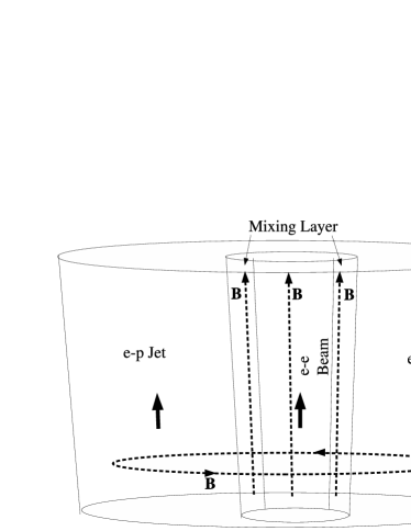
Figure 1: Two-fluid model for relativistic outflows. A fast, relativistic $e^{\pm}$ beam is surrounded by a slower, possibly thermal, $e^{-}p$ outflow, with a mixing layer forming between the beam and the jet. The magnetic field, $B$, is parallel to the flow in the beam and in the mixing layer, and the field is toroidal in the jet. The magnetic lines are perturbed and the perturbation propagates outwards at the Alfvén speed, $V_{\rm A}$.

2.1 Geometry of the model

Basic geometry of the model is illustrated in Fig. 2. Two black holes M₁ and M₂ orbit each other in the plane ($\chi$O$\zeta$). The center of the mass of the binary system is in O. An accretion disk around the black hole M₁ is inclined at an angle $\Omega_{\mathrm{p}}$ with respect to the orbital plane. The angle $\Omega_{\mathrm{p}}$ is the opening half-angle of the precession cone. The disk precesses around the $\tilde{\xi}$ axis, which is parallel to the $\xi$-axis. The momentary direction of the beam axis is then given by the vector $\@vec{{\mathrm{M}}_{1}{\mathrm{J}}}$. The line of sight makes an angle $\iota$ with the precession axis.

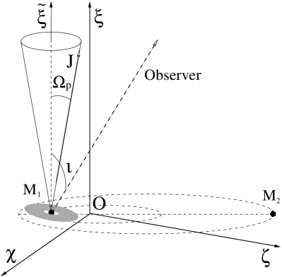
Figure 2: Geometry of the BBH model. M₁ and M₂ denote the locations of two black holes orbiting around each other in the plane ($\chi$O$\zeta$). The coordinate system is referenced to the center of mass of the binary system (O). The accretion disk around the black hole M₁ inclined at an angle $\Omega_{\mathrm{p}}$ with respect to the orbital plane, such that the $\tilde{\xi}$ axis (parallel to the $\xi$ axis) is the precession axis. The momentary direction of the beam axis is given by the vector $\@vec{{\mathrm{M}}_{1}{\mathrm{J}}}$.

2.2 Stability and dissipation of the beam

The beam exists inside the jet for as long as its density

$$n_{\mathrm{b}}\geq\varepsilon_{\mathrm{j}}/(\Gamma_{\mathrm{b}}^{2}m_{\mathrm{e}}c^{2})\,.$$ (1)

For a typical parsec-scale jet, this implies $n_{\mathrm{b}}\ga 10e^{-}\,\mathrm{cm}^{-3}$. The beam moves along magnetic field lines in the $e^{-}p$ jet if the magnetic field is larger than the critical value

$$B_{\mathrm{crit}}=(4\pi n_{\mathrm{mix}}m_{\mathrm{e}}c^{2})^{1/2}\,$$ (2)

where $n_{\mathrm{mix}}\approx n_{\mathrm{j}}$ is the density of the plasma in the beam–jet mixing layer (Pelletier, Sol & Asseo psa88 (1988)). The magnetic field in the jet rapidly becomes toroidal (Pelletier & Roland pr90 (1990)). The beam is not disrupted by Kelvin-Helmholtz perturbations if the magnetic field is larger than

$$B_{\mathrm{KH}}=(2\pi n_{\mathrm{b}}\Gamma_{\mathrm{b}}^{2}m_{\mathrm{e}}c^{2})^{1/2}$$ (3)

(Pelletier & Roland pr89 (1989)). A typical density ratio in parsec-scale jets is $\eta=(n_{\mathrm{b}}/n_{\mathrm{j}})\approxeq 0.01$, which implies $B_{\mathrm{crit}}\sim B_{\mathrm{KH}}\sim 50$ mG. Sol, Pelletier & Asseo (spa89 (1989)) have demonstrated that the beam does not suffer from inverse Compton and synchrotron losses on parsec scales. Relativistic bremsstrahlung, ionization and annihilation losses are also insignificant on these scales. Diffusion by turbulent Alfvén waves is not expected for beams with $\Gamma_{\mathrm{b}}\sim 10$.

2.3 Kinematics of the perturbed beam

The relativistic plasma injected into the beam in the vicinity of the black hole M₁ moves at a speed characterized by the bulk Lorentz factor $\Gamma_{\mathrm{c}}$. The condensation follows the magnetic field lines. The perturbation of the magnetic field propagates at the Alfvén speed $V_{\mathrm{A}}=B(4\pi m_{\mathrm{e}}n_{\mathrm{b}})^{-0.5}$. For highly energetic beams, the classical density $\rho_{0}=m_{\mathrm{e}}n_{\mathrm{b}}$ is substituted with the enthalpy $\mu=\rho+P/c^{2}$, where $P$ is the pressure, $\rho=\rho_{0}(1+\varepsilon/c^{2})$ is the relativistic density and $\varepsilon$ is the specific internal energy. Taking into account relativistic corrections, and recalling that the enthalpy becomes $\Gamma_{\mathrm{b}}(\rho+P/c^{2})$ in a plasma moving at a bulk speed $\beta_{\mathrm{b}}=(1-1/\Gamma_{\mathrm{b}}^{2})^{0.5}$, the resulting phase speed of the Alfvén perturbation with respect to the beam plasma is $V_{\mathrm{A,rel}}=\sqrt{1/(1+\Gamma_{\mathrm{b}}/V_{\mathrm{A}}^{2})}$. Thus, for a typical $e^{\pm}$ beam propagating at $\Gamma_{\mathrm{b}}\ga 10$ inside a jet with $B\ga B_{\mathrm{crit}}$, the relativistic Alfvén speed is $\approx 0.1\,c$.

The observed trajectory of the beam is affected primarily by the orbital motion in the BBH system and the precession of the AD around the primary BH. The jet structure on parsec scales is mainly determined by the precession. The orbital motion introduces a small ($\la 0.1$ mas) oscillation of the footpoint of the jet, and it is not immediately detectable in VLBI images with a typical resolution of $\approx 1$ mas. Consider first the effect of the precession of the accretion disk. The coordinates of the component moving in the perturbed beam are given by

$$\left\{\begin{split}\tilde{\chi}&=R(\xi)\cos(\omega_{\mathrm{p}}t-k_{\mathrm{p}}\xi+\phi_{\mathrm{p}})\\ \tilde{\zeta}&=R(\xi)\sin(\omega_{\mathrm{p}}t-k_{\mathrm{p}}\xi+\phi_{\mathrm{p}})\\ \tilde{\xi}&=\xi=\xi(t)\,,\end{split}\right.$$ (4)

where $R(\xi)$ is the perturbation amplitude, $\phi_{\mathrm{p}}$ is the initial precession phase, $T_{\mathrm{p}}$ is the precession period, $\omega_{\mathrm{p}}=2\pi/T_{\mathrm{p}}$ and $k_{\mathrm{p}}=\omega_{\mathrm{p}}/V_{\mathrm{A}}$. The time $t$ is measured in the rest frame of the beam. The tilde in $\tilde{\chi}$ and $\tilde{\zeta}$ indicates that the orbital motion has not yet been taken into account (here the axes $\tilde{\chi}$ and $\tilde{\zeta}$ are assumed to be parallel to the axes $\chi$ and $\zeta$, respectively; see Fig. 2). Obviously, $\tilde{\xi}=\xi$, and the tilde can be omitted in all expression with $\xi$. The $R(\xi)$ can be chosen to be

$$R(\xi)=\frac{R_{0}\xi}{a+\xi}\,.$$ (5)

Here, $a=R_{0}/(2\tan\Omega_{\mathrm{p}})$, and $R_{0}$ is the maximum amplitude of the perturbation.

The form of the function $\xi(t)$ depends on the evolution of the speed $\beta_{\mathrm{c}}$ of the plasma condensation injected into the perturbed beam. From Eq. (4), the components of $\beta_{\mathrm{c}}$ are:

$$\left\{\begin{split}\beta_{\tilde{\chi}}=&\;\beta_{\xi}({\mathrm{d}}R/{\mathrm{d}}\xi)\cos(\omega_{\mathrm{p}}t-k_{\mathrm{p}}\xi+\phi_{\mathrm{p}})-\\ &-R(\xi)\,(\omega-k\beta_{\xi})\sin(\omega_{\mathrm{p}}t-k_{\mathrm{p}}\xi+\phi_{\mathrm{p}})\\ \beta_{\tilde{\zeta}}=&\;\beta_{\xi}({\mathrm{d}}R/{\mathrm{d}}\xi)\sin(\omega_{\mathrm{p}}t-k_{\mathrm{p}}\xi+\phi_{\mathrm{p}})+\\ &+R(\xi)\,(\omega-k\beta_{\xi})\cos(\omega_{\mathrm{p}}t-k_{\mathrm{p}}\xi+\phi_{\mathrm{p}})\\ \beta_{\tilde{\xi}}=&\;\beta_{\xi}={\mathrm{d}}\xi/{\mathrm{d}}t\,,\end{split}\right.$$ (6)

so that

$$\beta^{2}_{\mathrm{c}}=({\mathrm{d}}\xi/{\mathrm{d}}t)^{2}C_{1}+R^{2}(\xi)\,(\omega_{\mathrm{p}}-k_{\mathrm{p}}{\mathrm{d}}\xi/{\mathrm{d}}t)^{2}\,,$$ (7)

where $C_{1}=({\mathrm{d}}R/{\mathrm{d}}\xi)^{2}+1$, and remembering that $\beta_{\mathrm{c}}^{2}=\beta_{\tilde{\chi}}^{2}+\beta_{\tilde{\zeta}}^{2}+\beta_{\tilde{\xi}}^{2}$. Equation (7) is a quadratic equation with respect to ${\mathrm{d}}\xi/{\mathrm{d}}t$, and it can be written in the form of

$$A_{2}({\mathrm{d}}\xi/{\mathrm{d}}t)^{2}+A_{1}({\mathrm{d}}\xi/{\mathrm{d}}t)+A_{0}=0\,,$$ (8)

with $A_{2}=1+R^{2}(\xi)k^{2}_{\mathrm{p}}+({\mathrm{d}}R/{\mathrm{d}}\xi)^{2}$, $A_{1}=-2R^{2}(\xi)\omega_{\mathrm{p}}k_{\mathrm{p}}$ and $A_{0}=R^{2}(\xi_{\mathrm{c}})\omega^{2}_{\mathrm{p}}-\beta^{2}_{\mathrm{c}}$. The component speed $\beta_{\mathrm{c}}$ can be conveniently expressed as a function of $\xi$ or $\xi(t)$ (it can also be viewed constant, in the simplest case). The jet side solution of Eq. (7) can be obtained for the time $t(\xi)$ in the rest frame of the beam, under the condition of initial acceleration of the beam (${\mathrm{d}}\xi/dt>0$, for $\xi\rightarrow 0_{+}$). The formal solution of Eq. (8) is

$$\begin{split}\frac{{\mathrm{d}}\xi}{{\mathrm{d}}t}=&\;\frac{1}{A_{2}}\{R^{2}(\xi)\omega_{\mathrm{p}}k_{\mathrm{p}}+\\ &\;+\left[R^{2}(\xi)k^{2}_{\mathrm{p}}\beta^{2}_{\mathrm{c}}+(\beta^{2}_{\mathrm{c}}-R^{2}(\xi)\omega^{2}_{\mathrm{p}})(1+\frac{{\mathrm{d}}R}{{\mathrm{d}}\xi})\right]^{1/2}\}\,,\\ \end{split}$$ (9)

and $t(\xi)$ is then given by

$$\begin{split}t(\xi)&=t_{0}+\int^{\xi}_{\xi_{0}}\frac{A_{2}}{k_{\mathrm{p}}\omega_{\mathrm{p}}R^{2}(\xi)+[A_{2}\beta^{2}_{\mathrm{c}}-\omega^{2}_{\mathrm{p}}R^{2}(\xi)C_{1}]^{1/2}}{\mathrm{d}}\xi\,.\\ \end{split}$$ (10)

In general, both $\omega_{\mathrm{p}}$ and $k_{\mathrm{p}}$ can also vary. Their variations should then be given with respect to $\xi$, in order to preserve the solution given by Eq. (10). Numerical methods should be used otherwise. The solution determined by Eq. (10) can be found for all $R(\xi)$ not exceeding the limit of

$$R(\xi)\leq\beta_{\mathrm{c}}\left[\omega^{2}_{\mathrm{p}}-k^{2}_{\mathrm{p}}\beta^{2}_{\mathrm{c}}\cos^{2}\psi(\xi)\right]^{-1/2}$$ (11)

The beam pitch angle $\psi(\xi)=\arctan({\mathrm{d}}R/{\mathrm{d}}\xi)$ in Eq. (11) is measured “locally” (as opposed to the “global” pitch angle $\psi_{\mathrm{g}}(\xi)=\arctan[R(\xi_{\mathrm{c}})/\xi]$), and it describes the evolution of the amplitude of the beam perturbation. For a jet with constant beam pitch angle ($\psi(\xi)=\psi=const$), the inequality 11 can be rewritten as:

$$\xi\leq\beta_{\mathrm{c}}\left[\omega^{2}_{\mathrm{p}}\tan^{2}\psi-k^{2}_{\mathrm{p}}\beta^{2}_{\mathrm{c}}\sin^{2}\psi\right]^{-1/2}$$ (12)

The speed $\beta_{\mathrm{c}}$ and the local pitch angle $\psi$ should satisfy the condition:

$$\beta_{\mathrm{c}}\cos\psi\leq\frac{V_{\mathrm{A}}}{({V^{2}_{\mathrm{A}}+1})^{0.5}}\,,$$ (13)

If inequalities 11–13 are satisfied, the solution provided by Eq. (10) can be used to represent the form of the function $\xi(t)$ and describing the kinematics of the beam.

2.4 The binary system

The trajectory of a superluminal feature travelling in the perturbed beam is modified also by the orbital motion of the two black holes in the binary system. This motion can be taken into account by solving the restricted three-body problem for the BBH–AD system (Laskar las90 (1990), Laskar & Robutel lr95 (1995)). The orbital plane is $(\chi O\zeta)$, and the coordinate system is centered at the mass center of the system. The orbit is given by $r=p/[1+e\,\cos\varphi(t)]$, where $\varphi$ is the true anomaly, $p$ is the semi-latus rectum and $e$ is the numerical eccentricity of the orbit. The resulting coordinates ($\chi_{1}$, $\zeta_{1}$) of the black hole M₁ are given by

$$\left\{\begin{split}\chi_{1}(t)&=\frac{M_{2}}{M_{1}+M_{2}}\frac{p}{1+e\cos(\varphi(t))}\cos(\varphi(t))\\ \zeta_{1}(t)&=\frac{M_{2}}{M_{1}+M_{2}}\frac{p}{1+e\cos(\varphi(t))}\sin(\varphi(t))\end{split}\right.$$ (14)

The beam trajectory can be reconstructed from Eqs. (4) and (14), which gives

$$\left\{\begin{split}\chi&=\tilde{\chi}+\chi_{1}(t)\cos(\omega_{\mathrm{o}}t-k_{\mathrm{o}}\xi(t)+\phi_{\mathrm{o}})\\ \zeta&=\tilde{\zeta}+\zeta_{1}(t)\sin(\omega_{\mathrm{o}}t-k_{\mathrm{o}}\xi(t)+\phi_{\mathrm{o}})\\ \xi&=\xi(t)\end{split}\right.$$ (15)

where $\phi_{\mathrm{o}}$ is the initial orbital phase, $\omega_{\mathrm{o}}=2\pi/T_{\mathrm{o}}$, $k_{\mathrm{o}}=\omega_{\mathrm{o}}/V_{\mathrm{A}}$, and $T_{\mathrm{o}}$ is the orbital period. This system of equations describes completely the kinematics of the perturbed beam. Similarly to the solution obtained for Eq. (8), $\xi(t)$ can now be determined by forming $\beta_{\mathrm{c}}^{2}$ from the coordinate offsets given by Eq. (15) and solving for ${\mathrm{d}}\xi/{\mathrm{d}}t$, so that (for the jet side solution)

$$t(\xi)=t_{0}+\int_{\xi_{0}}^{\xi}\frac{2A_{2}}{({A_{1}}^{2}-4A_{1}A_{0})^{1/2}-A_{1}}{\mathrm{d}}\xi$$ (16)

The coefficients $A_{0}$, $A_{1}$, and $A_{2}$ are given explicitly in Appendix II in Britzen et al. (bri+01 (2001)).

2.5 Properties of the $t(\xi)$ solution

The strongest effect on the form of the beam trajectory is produced by three model parameters: the beam speed $\beta_{\mathrm{c}}$, the Alfvén speed $V_{\mathrm{A}}$, and the precession period $T_{\mathrm{p}}$. The orbital period in the BBH system affects only the position of the footpoint of the jet. Since VLBI measurements are made with respect to the footpoint position, $T_{\mathrm{o}}$ would not have an effect on fitting the observed trajectories of the jet components (the orbital period is constrained by the variability of the optical emission). It is easy to see that the remaining parameters ($R_{0}$, $\Omega_{\mathrm{p}}$, $\iota$ and $\theta$) describe only the orientation and shape of the overall envelope within which the perturbed beam is evolving. The $t(\xi)$ solutions described by Eqs. (10) and 16 can degenerate or become non-unique with respect to $\beta_{\mathrm{c}}$, $V_{\mathrm{A}}$, $T_{\mathrm{p}}$, if these parameters are correlated. The combinations of $\beta_{\mathrm{c}}$, $T_{\mathrm{p}}$ and $V_{\mathrm{A}}$ describing the same beam trajectory must not depend on the rest frame time $t$ or beam location $\xi$. However, the solution given by equation 10 implies that the beam trajectory would remain the same if

$$T_{\mathrm{p}}=\frac{2\pi R_{0}\xi(\xi-V_{\mathrm{A}}t)}{(a+\xi)(\beta^{2}_{\mathrm{c}}t^{2}-\xi^{2})^{1/2}V_{\mathrm{A}}}\,.$$ (17)

Obviously, Eq. (17) depends on both $t$ and $\xi$. The dependence vanishes only when $t\rightarrow\xi/c$. The precession period then becomes a complex number, and the resulting combination of the parameters does not describe a physically meaningful situation. This implies that the model does not become degenerate or non-unique with respect to $\beta_{\mathrm{c}}$, $T_{\mathrm{p}}$ and $V_{\mathrm{A}}$, and each physically possible combination of these parameters describes a unique beam trajectory.

2.6 Specific properties of the model

The model introduces two new properties in the description of the BBH–AD system: 1) the Lorentz factor of the relativistic beam is time variable; 2) the initial perturbation of the magnetic lines in the beam dissipates on a timescale $t_{\mathrm{beam}}$. These modifications are introduced in order to accommodate for the kinematic properties of the jet in 3C 345 in which the curvature of component trajectories decreases at larger distances, and accelerated motions are strongly implied by the observed trajectories and apparent speeds of several jet components (LZ (99)). The beam accelerates from $\Gamma_{\mathrm{min}}$ to $\Gamma_{\mathrm{max}}$ over a rest frame time interval $t_{\mathrm{acc}}$, and

$$\Gamma_{\mathrm{c}}(t)=\frac{\Gamma_{\mathrm{min}}+\Gamma_{\mathrm{max}}(t/t_{\mathrm{acc}})}{1+t/t_{\mathrm{acc}}}\;.$$ (18)

The perturbation dissipates at a characteristic time $t_{\mathrm{beam}}$. The amplitude of the perturbation given by equation (5) is modified by an attenuation term (characteristic damping time of the perturbation), so that

$$R(\xi)=\frac{R_{0}\xi}{a+\xi}\,e^{-t/t_{\mathrm{beam}}}\;.$$ (19)

The model takes account of an arbitrary source orientation, by introducing a position angle, $\Theta_{\xi}$ of the $\xi$-axis in the picture plane of the observer.

2.7 Observed quantities

Corrections for the relativistic motion of the beam must be made, in order to enable calculations of physical quantities in the observer’s frame. This requires a knowledge of the angle $\theta(t)$ between the instantaneous velocity vector of the component and the line of sight (LOS). Since the observed angular size of the BBH orbit is small ($\ll 1$ milliarcsecond), the LOS can be assumed to lie in the plane parallel to $(\chi O\xi)$, making an angle $\iota$ with the $\xi$ axis. In this case,

$$\cos\theta(t)=\left(\frac{{\mathrm{d}}\chi}{{\mathrm{d}}t}\sin\iota+\frac{{\mathrm{d}}\xi}{{\mathrm{d}}t}\cos\iota\right)\frac{1}{\beta_{\mathrm{c}}}$$ (20)

in the observer’s frame (Camenzind & Krockenberger ck92 (1992)), with the resulting Doppler beaming factor $\delta_{\mathrm{c}}(t)=\{\Gamma_{\mathrm{c}}[1-\beta_{\mathrm{c}}\cos\theta(t)]\}^{-1}$ The observed flux density of the moving component is

$$S_{\mathrm{c}}=\frac{1}{D^{2}_{\mathrm{L}}}\delta_{\mathrm{c}}(t)^{1+\alpha_{\mathrm{s}}}(1+z)^{1+\alpha_{\mathrm{s}}}\int_{\mathrm{c}}j_{\mathrm{c}}{\mathrm{d}}V\,,$$ (21)

where $z$ and $D_{\mathrm{L}}$ are the redshift and luminosity distance of the source, $j_{\mathrm{c}}$ is the emissivity of the component and $\alpha_{\mathrm{s}}$ is the synchrotron spectral index. The shortening of time in the observer’s frame is given by

$$t_{\mathrm{obs}}=(1+z)\int_{0}^{t}\frac{{\mathrm{d}}t}{\Gamma_{\mathrm{c}}(t)\delta_{\mathrm{c}}(t)}\,,$$ (22)

and the component travels over the distance

$$R_{\mathrm{trav}}(t)=(1+z)^{-1}\int_{0}^{t}\frac{\beta_{\mathrm{c}}}{1-\beta_{\mathrm{c}}\cos\theta(t)}{\mathrm{d}}t\,.$$ (23)

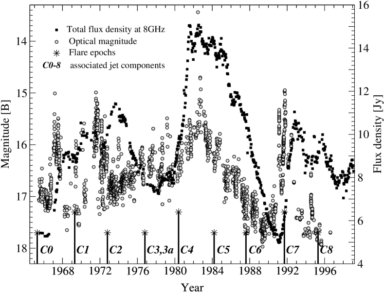
Figure 3: Optical and radio variability of 3C 345. Shown are the epochs of spectral flares (LZ (99)) that have resulted in appearances of new superluminal components in the jet. The radio data are from the Michigan monitoring program ( Aller, Aller & Hughes aller03 (2003)). The optical data are from Kinman et al. (kin+68 (1968)); Smyth & Wolstencroft (sw70 (1970)); Lü (lu72 (1972)); McGimsey et al. (mcg+75 (1975)); Pollock et al. (pol+79 (1979)); Angione et al. (ang+81 (1981)); Kidger (kid88 (1988)) Webb et al. (web+88 (1988)); Kidger & de Diego (990 ); Vio et al (vio+91 (1991)); Schramm et al. (sch+93 (1993)); Babadzhanyants, Belokon’ & Gamm (bbg95 (1995)); Belokon’ & Babadzhanyants (bb99 (1999)). All optical data have been converted into the B magnitude scale.

3 The quasar 3C 345

The 16^m quasar 3C 345 exhibits remarkable structural and emission variability on parsec scales around a compact unresolved radio core. The total radio flux density of 3C 345 has been monitored at 5, 8, and 15 GHz (Aller, Aller & Hughes aller03 (2003)), and at 22 and 37 GHz (Teräsranta et al. ter+98 (1998)). The source has also been monitored with the Green Bank Interferometer at 2.7 and 8.1 GHz (Waltman et al. wal+91 (1991)). The observed variability of the optical emission is possibly quasi-periodic with a period of $\approx$1560 days (Babadzhanyants & Belokon’ 1984; Kidger 1989), although it has been suggested that the light curve may originate from a non-linear and non-stationary stochastic process (Vio et al. vio+91 (1991)). A strong optical flare observed in 3C 345 in 1991–92 (Schramm et al. sch+93 (1993); Babadzhanyants, Belokon’ & Gamm bbg95 (1995)) was connected with the appearance of a new superluminal jet component, C7 (L (96)). LZ (99) report possible 3.5–4 year quasi-periodicity manifested by spectral flares of the radio emission and appearances of new jet components. Historical optical and 8 GHz radio lightcurves are shown in Fig. 3 together with the epochs of the spectral flares and component ejections.

The evolution of the parsec-scale jet of 3C 345 has been studied extensively with the VLBI: see Unwin et al. (unw+83 (1983)); Biretta, Moore & Cohen (bmc86 (1986)); Zensus, Cohen & Unwin (1995, hereafter ZCU (95)); L (96); Ros, Zensus & Lobanov (2000, hereafter R (00)); Klare (kla03 (2003)). The relativistic jet model (Blandford & Rees br78 (1978)) has been applied to explain the emission and kinematic changes observed in the parsec-scale structures. Using the X-ray data to constrain the jet kinematics, ZCU (95) and Unwin et al. (unw+94 (1994)) derive physical conditions in the jet from a model that combines the inhomogeneous jet model of Königl (kon81 (1981)) for the core with homogeneous synchrotron spheres for the moving jet components (Cohen coh85 (1985)). The evolution of the core flux density is well represented by a sequence of flare-type events developing in a partially opaque, quasi-steady jet (LZ (99)). Spectral properties of the parsec-scale emission have been studied in several works (L (96); Lobanov, Carrara, & Zensus lcz97 (1997); Lobanov 1998b ). Unwin et al. (unw+97 (1997)) have analyzed a correlation between the X-ray variability and parsec-scale radio structure of 3C 345.

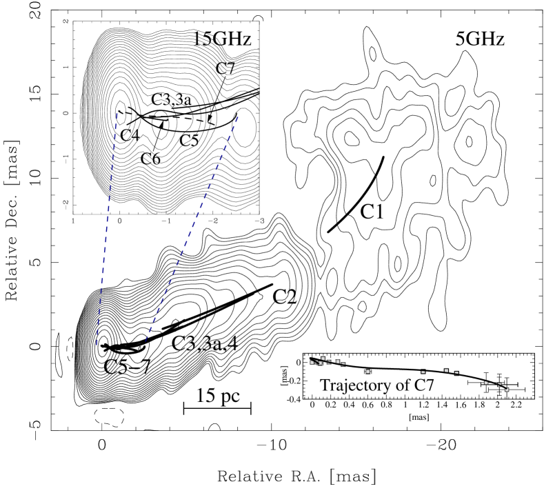
Figure 4: Parsec-scale jet in 3C 345 at 5 and 15 GHz. Contours are drawn at -1,1,$\sqrt{2}$,2,… of the lowest contour (2.5 mJy/beam, in both images). Curved lines mark the trajectories of superluminal features C1–C7 identified in the jet. The component trajectories are polynomial fits to the position measurements from the 1979–1998 VLBI monitoring data (ZCU (95); L (96); R (00)). The positions of C7 measured at 22 GHz are shown in the inset.

Table 1: Positions and flux densities of C7 at 22 GHz

$t_{\mathrm{obs}}$	$S$	$\Delta x$	$\Delta y$
$[{\mathrm{y}ear}]$	$[{\mathrm{J}y}]$	$[{\mathrm{m}as}]$	$[{\mathrm{m}as}]$
1989.25†	$0.19\pm 0.02$	$0.04\pm 0.02$	$0.01\pm 0.01$
1991.46	$0.80\pm 0.04$	$0.09\pm 0.05$	$-0.01\pm 0.01$
1991.86	$3.29\pm 0.49$	$0.12\pm 0.01$	$0.03\pm 0.01$
1992.45	$6.20\pm 0.36$	$0.18\pm 0.01$	$0.00\pm 0.01$
1992.86	$5.49\pm 0.30$	$0.28\pm 0.01$	$0.01\pm 0.01$
1993.13	$3.60\pm 0.10$	$0.34\pm 0.01$	$-0.02\pm 0.01$
1993.72	$2.23\pm 0.12$	$0.60\pm 0.04$	$-0.10\pm 0.02$
1994.45	$1.04\pm 0.10$	$0.90\pm 0.09$	$-0.12\pm 0.08$
1995.85	$1.21\pm 0.06$	$1.20\pm 0.08$	$-0.10\pm 0.08$
1996.42	$0.88\pm 0.05$	$1.36\pm 0.08$	$-0.07\pm 0.07$
1996.82	$0.69\pm 0.04$	$1.55\pm 0.08$	$-0.08\pm 0.12$
1997.40	$0.64\pm 0.10$	$1.87\pm 0.10$	$-0.22\pm 0.13$
1997.62	$0.59\pm 0.07$	$2.02\pm 0.10$	$-0.24\pm 0.12$
1997.90	$0.47\pm 0.07$	$2.10\pm 0.10$	$-0.30\pm 0.11$
1998.02	$0.47\pm 0.08$	$2.02\pm 0.25$	$-0.24\pm 0.14$
1998.99	$0.50\pm 0.10$	$2.63\pm 0.20$	$-0.15\pm 0.14$
1999.12	$0.28\pm 0.10$	$2.69\pm 0.20$	$-0.36\pm 0.14$
1999.64	$0.17\pm 0.20$	$2.87\pm 0.20$	$-0.34\pm 0.15$

Note: ${\dagger}$ – detection is likely to be confused due to blending between the core and the preceeding jet component C6. References: 1989.25–1993.72 (L (96)); 1994.45 (Leppänen, Zensus & Diamond lzd95 (1995)); 1996.42–1997.40 (R (00)); 1997.62–1999.64 (Klare kla03 (2003)).

3.1 Compact jet in 3C 345

Figure 4 shows VLBI images of the jet in 3C 345 at 5 and 15 GHz, with the trajectories of eight superluminal components identified and monitored in the jet in 1979–1999. The morphology of 3C 345 is typical for a core dominated source: a bright and compact core responsible for 50–70% of the total emission, and a compact jet that contains several enhanced emission regions (jet components) moving at apparent speeds of up to $\beta_{\mathrm{{app}}}\approx 20h^{-1}$.

The compact jet in 3C 345 extends over $\sim 25$ mas, which corresponds to a projected distance of $\approx$95$\,(h\,\sin\theta_{\mathrm{jet}})^{-1}$ pc ($\approx$800 $h^{-1}$ pc, assuming the most likely viewing angle of the jet $\theta_{\mathrm{jet}}=7\degr$) . The jet has two twists at the separations of $\approx$1 and $\approx$5 mas. The twists appear to retain their positions in the jet over the entire duration of the VLBI monitoring. Such stability of the twists suggests that they are likely to reflect the three-dimensional structure of the jet. The unchanging positions of the twists are also consistent with the similarities of the apparent trajectories of the jet components at separations $\geq$1 mas (Fig. 4). The two-dimensional trajectories observed in several jet components follow similar, overlapping tracks, and outline a continuous picture of a curved jet. The separation of 20 mas from the core can mark a transition point from compact jet to large-scale jet. At this separation, the jet finally turns to the direction $\phi\approx-40\degr$ observed in the large-scale jet of 3C 345 (Kolgaard, Wardle & Roberts kwr89 (1989)).

The measured positions of the component C7 (Fig. 4) provide an accurate account of the jet kinematics within $\sim$2 mas distance from the core. The large amount and good quality of the data at 22 GHz are sufficient for determining the component trajectory without using measurements made at lower frequencies. The total of 18 VLBI observations of 3C 345 at 22 GHz are combined for the epochs between 1989 and 1998 (L (96); R (00); Klare kla03 (2003)). For several of these observations, new model fits have been made for the purpose of obtaining consistent error estimates for the positions and flux densities of C7. Table 1 presents the resulting database of the positions and flux densities of C7 at 22 GHz.

C7 was first reliably detected in 1991.5 at 22 GHz at a core separation of $\Theta_{1991.5}\approx 100\,\mu$as (L (96)) Reports of earlier detections in 1989.2 at 100 GHz (Bååth et al. baa+92 (1992)) and 22 GHz (L (96)) are inconclusive because of the likely confusion and blending with the nearby component C6 and the core itself.

Following the procedure established in ZCU (95) and L (96), polynomial functions are fitted to the component coordinate offsets $x(t)$ and $y(t)$ from the core position which is fixed at the point (0,0). From the polynomial fits, the proper motion $\mu(t)=[({\mathrm{d}}x/{\mathrm{d}}t)^{2}+({\mathrm{d}}y/{\mathrm{d}}t)^{2}]^{1/2}$, apparent speed $\beta_{\mathrm{app}}(t)=\mu(t)D_{\mathrm{L}}(1+z)^{-1}$ and apparent distance ${\Theta}_{app}(t)=\int\mu(t^{\prime})dt^{\prime}$ travelled by the component along its two-dimensional path can be recovered. For the purpose of comparison to the previous work of L96 and Lobanov & Zensus (lz96 (1996)), the detection reported for the epoch 1989.25 is included in the polynomial fitting, but all results for the epochs before 1991 should be viewed as only tentative.

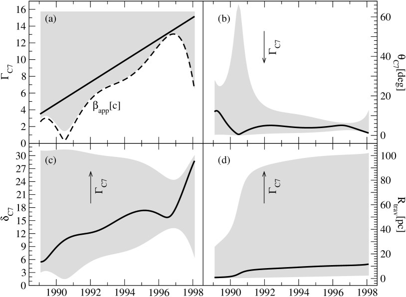
Figure 5: Kinematic properties of the jet determined from the observed trajectory of C7. In all panels, the solid line represents a model with $\Gamma_{\mathrm{C7}}$ increasing linearly with time from $\Gamma_{\mathrm{C7}}=2.2$ in 1990 to $\Gamma_{\mathrm{C7}}=10.6$ in 1998. The lower boundary of the shaded area corresponds to $\Gamma_{\mathrm{C7}}=\Gamma_{\mathrm{min}}=(\beta_{\mathrm{app}}^{2}+1)^{1/2}$, the upper boundary is drawn for $\Gamma_{\mathrm{C7}}=11$. Arrows indicate the direction of increasing $\Gamma_{\mathrm{C7}}$ from $\Gamma_{\mathrm{min}}$ to 11. Individual panels show: (a) Measured apparent speed $\beta_{\mathrm{app}}$ (dashed line) and evolution of the Lorentz factor $\Gamma_{\mathrm{j}}$. (b) Angle between the velocity vector of C7 and the line of sight. (c) Doppler factor. (d) Distance travelled by C7 in the rest frame of the jet. The derived $R_{\mathrm{trav}}>\beta_{\mathrm{C7}}\Delta t_{\mathrm{obs}}$ because of the time contraction in the observer’s frame of reference.

3.2 Kinematics of the jet component C7

Kinematic properties of C7 are presented in Fig. 5. The apparent speed $\beta_{\mathrm{app}}$ of C7 increased from $\approx 2\,c$ in 1989 to $\beta_{\mathrm{max}}\approx 13\,c$ in 1997 (the decrease of $\beta_{\mathrm{app}}$ after 1997 is an artifact of the polynomial fit). The component reached the minimum apparent speed of $\beta_{\mathrm{min}}\approx 0.5\,c$ in 1990.5. Such large changes of $\beta_{\mathrm{app}}$ indicate that C7 has moved along a substantially curved three-dimensional path, with the bulk Lorentz factor most likely changing with time. If the Lorentz factor is constant, then $\Gamma_{\mathrm{C7}}>13$ (to satisfy the observed $\beta_{\mathrm{app}}$). If $\Gamma_{\rm mathrmC7}$ varies, the lower boundary of the variations is given by the minimum Lorentz factor $\Gamma_{\mathrm{min}}=[\beta_{\mathrm{app}}^{2}(t)+1]^{1/2}$, which describes the motion with the least kinetic power. In Fig. 5, $\Gamma_{\mathrm{max}}=15.5$ is set, and the kinematic parameters of C7 are described for all allowed variations of $\Gamma_{\mathrm{C7}}(t)$ ($\Gamma_{\mathrm{min}}(t)\leq\Gamma_{\mathrm{C7}}(t)\leq\Gamma_{\mathrm{max}}$). As seen in Fig. 5, neither of the two boundaries provides a satisfactory description of the component kinematics. The case $\Gamma_{\mathrm{C7}}=\Gamma_{\mathrm{max}}$ results in uncomfortably small $\theta_{\mathrm{C7}}(t)$ and disproportionally large travelled distance $R_{\mathrm{trav}}(t)$. With $\Gamma_{\mathrm{C7}}=\Gamma_{\mathrm{min}}(t)$, the resulting variations of $\theta_{\mathrm{C7}}$ exceed $50\degr$, which is difficult to explain. A plausible evolution of the rest frame speed of C7 can be described by a linear increase of the Lorentz factor from $\Gamma_{\mathrm{C7}}=2.2$ in 1989 to $\Gamma_{\mathrm{C7}}=15$ in 1998. In this case, none of the kinematic parameters change drastically in the course of the component evolution: $\theta_{\mathrm{C7}}$ varies within $\approx 10\degr$, and $R_{\mathrm{trav}}\leq 10$ pc. This indicates that the motion of C7 is likely to be accelerated during the initial stages of its evolution, at distances of $\leq 2$ mas from the core. At such distances, acceleration of the component rest frame speeds has also been reported in several other jet components in 3C 345 (Lobanov & Zensus lz96 (1996), LZ (99)). Consequently, this must be a general property of the jet plasma on these spatial scales, and it should be taken into account in the modelling of the jet kinematics.

3.3 Long term trends in the jet: evidence for precession

The observed consistency of the two-dimensional component tracks plotted in Fig. 4 suggests that all jet components in 3C 345 travel along similar trajectories. There is however a substantial amount of evidence for global evolution of the entire jet. In Fig. 6, the apparent accelerations, ${\mathrm{d}}\mu/{\mathrm{d}}\Theta_{\mathrm{app}}$, of the components are plotted against the respective component origin epochs taken from L (96). The apparent accelerations show a steady increase, following the order of component succession, which is a strong indication for long-term changes in the jet. While it is conceivable that the younger components are intrinsically faster, this would require the presence of a non-stationary process affecting significantly the particle acceleration in the nuclear regions of 3C 345. The more likely explanation of the observed long-term trend of the component accelerations is precession of the jet axis. In this case, variations of the component ejection angle alone are sufficient to explain the observed trend: the components ejected at angles closer to $\theta_{\mathrm{fast}}=1/\Gamma_{\mathrm{b}}$ would have higher ${\mathrm{d}}\mu/{\mathrm{d}}\Theta_{\mathrm{app}}$. In the course of the precession, the ejection angle would change steadily, and the measured ${\mathrm{d}}\mu/{\mathrm{d}}\Theta_{\mathrm{app}}$ should show sinusoidal variations. The rather large errors in the measured ${\mathrm{d}}\mu/{\mathrm{d}}\Theta_{\mathrm{app}}$ in Fig. 6 allow only a very rough estimate of the precession period $T_{\mathrm{prec}}$, which should be in the range of 850–3670 years, to be made.

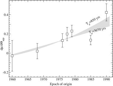
Figure 6: Apparent acceleration ${\mathrm{d}}\mu/{\mathrm{d}}\Theta_{\mathrm{app}}$ of the component proper motions, plotted versus the component epochs of origin. The origin epochs are obtained by back-extrapolating the observed trajectories of the jet components (L (96)). The shaded area cover the range of precession periods which would reproduce the observed trend of ${\mathrm{d}}\mu/{\mathrm{d}}\Theta_{\mathrm{app}}$.

Periodic changes are also evident in the variations of the jet position angle measured at 22 GHz for successive jet components as they reach a $\approx$0.5 mas separation from the core. The resulting position angles are plotted in Fig. 7. The position angle varies with a period of $P_{\mathrm{short}}\approx$9.5 years and an amplitude of $A_{\mathrm{short}}\approx$20$\degr$. A longer term trend is suggested by the slope in the linear regression of the position angle data, which implies a rate of change in the position angle of $\approx$0.4$\degr$/year. The time coverage of the data is too short to provide an accurate estimate of the period of the long term variations. A formal fit constrains the period to within a range of 300–3000 years, with a mean value of $P_{\mathrm{long}}\approx 1600$ years and an amplitude of $A_{\mathrm{long}}\approx 10\degr$. The shaded area in Fig. 7 represents a combined fit to the data by the two periods. The estimate of $P_{\mathrm{long}}$ obtained from the change in position angle falls within the range of periods implied by ${\mathrm{d}}\mu/{\mathrm{d}}\Theta_{\mathrm{app}}$, and it can therefore be associated with the precession. The nature of the short-term changes of the jet position is unclear, but they could be related to the rotation of the accretion disc or the jet itself or to the orbital motion in the BBH system.

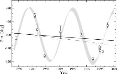
Figure 7: Position angle of different jet components measured at 22 GHz at 0.5 mas separation from the core. Short-term variations, with a period of $\approx$9.5 years, are evident. A linear regression (dotted line) suggests the presence of a long-term trend, with a annual change rate of 0.4$\pm$0.3$\degr$/year. The shaded area shows the best fit by the two periodical processes combined, with the estimated periods $P_{\mathrm{short}}=9.5\pm 0.1$ years and $P_{\mathrm{long}}=1600\pm 1300$ years. The solid line represents the trend in the position angle due to the long-term periodicity.

4 Application of the BBH model

The BBH model applies a single model framework to explain the emission and kinematic properties of the jet in the optical and radio regimes. The evolution of superluminal features observed in the radio jet is explained by a precession of the accretion disk around the primary black hole M₁, and the characteristic shape of the optical light curve is produced by the orbital motion of the black hole M₁.

The different characteristic timescales and amplitudes of changes in the radio and optical regimes imply a complex composition of the emitting material. The optical emission of 3C 345 during the strong flare in 1990–93 varied by $\approx 2.5$ mag, with a typical timescale of $\sim$0.6 yr for individual sub-flare events (see Fig. 15). The radio emission of the jet component C7 associated with that flare showed only a single rise and decay event, changing by a factor of $\sim$15 on a timescale of $\sim$6 years. This difference in the behavior of the optical and radio variability can be reconciled by assuming that the relativistic $e^{\pm}$ plasma responsible for the optical emission is injected into the beam during a time $\Delta\tau_{\mathrm{opt}}$ which is much shorter than the injection timescale $\Delta\tau_{\mathrm{rad}}$ for the plasma responsible for the radio emission. For C7, the plasma responsible for the optical emission is modelled by a point-like component and the plasma responsible for the radio emission is modelled by a temporally extended component, so that $\Delta\tau_{\mathrm{opt}}<0.01\Delta\tau_{\mathrm{rad}}$. In the BBH frame, the radio component emits over a period of $\approx 1.9$ yr, with component ejections occurring approximately every 4 years. A general sketch of the composition of a flare is shown in Fig. 8.

The application of the model consists of two parts. In the first part, the observed trajectory and flux density of the jet component C7 are reconstructed, using the precession of the accretion disk around the black hole M₁, and solving formally the problem defined by Eq. (8). In the second part, the optical light curve of 3C 345 is calculated from the orbital properties of the BBH system provided by the solution of Eq. (16).

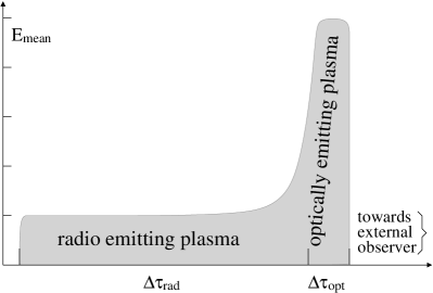
Figure 8: Composition of a nuclear flare. The flare begins with an injection of highly energetic particles emitting optical synchrotron radiation. The timescale of the injection $\Delta\tau_{\mathrm{opt}}$ is comparable to the synchrotron loss time of the optically emitting plasma. Rapid energy losses and injection of radio emitting plasma on the timescale $\Delta\tau_{\mathrm{rad}}$ lead to progressively decreasing mean energy of the plasma and subsequent propagation of the flare to radio wavelengths. The optically emitting plasma is represented in the model by a point-like component injected into the beam, while the radio emitting plasma is temporally resolved, with the resulting $\Delta\tau_{\mathrm{opt}}<0.01\Delta\tau_{\mathrm{rad}}$

4.1 Precession and geometry

Basic geometrical parameters of the system are recovered by fitting the precession model to the observed two-dimensional path of C7. These include

$\iota$ – viewing angle of the jet axis (Fig. 2);

$\Psi_{\mathrm{proj}}$ – position angle of the jet axis in the plane of the sky;

$T_{\mathrm{p}}$ – precession period;

$\Omega_{\mathrm{p}}$ – opening half-angle of the precession cone;

$\phi_{\mathrm{p}}$ – initial phase of the precession;

$R_{0}$ – maximum amplitude of the perturbation;

$t_{\mathrm{beam}}$ – characteristic dampening time of the perturbed beam.

It should be stressed that none of the parameters listed above depend on the velocity of the moving component. However, the shape of the path depends on the Alfvén speed $V_{\mathrm{A}}$ of the magnetic field perturbation. This speed is determined by fitting simultaneously the geometry of the component path and the orbital motion in the binary system.

4.1.1 Velocity of the jet component

The velocity of the jet component is constrained by fitting the coordinate offsets, $x(t)$ and $y(t)$, of the component from the position of the radio core. In 3C 345, the apparent motion of all jet components is non-linear and shows accelerations and decelerations (ZCU (95); L (96); LZ (99)). To account for this, a variable Lorentz factor must be introduced, using Eq. (18). With a variable Lorentz factor, the $x(t)$ and $y(t)$ offsets are fitted simultaneously, and a three-dimensional trajectory of the component is recovered. This procedure yields the following parameters:

$\Gamma_{\mathrm{min}}$ – initial Lorentz factor of the component;

$\Gamma_{\mathrm{max}}$ – final Lorentz factor of the component, after the acceleration;

$t_{\mathrm{acc}}$ – characteristic acceleration time.

4.2 Flux density changes in the jet component

In addition to the geometrical and kinematic factors, the flux density evolution in the optical and radio regimes is characterized by the synchrotron energy loss timescales $\Delta\tau_{\mathrm{opt}}$ and $\Delta\tau_{\mathrm{rad}}$ and by the duration $\Delta\tau_{\mathrm{thick}}$ during which the relativistic plasma responsible for the flare remains optically thick in the radio regime. The radio lightcurve of C7 constrains uniquely the viewing angle of the jet. The information contained in the radio lightcurve is fundamental for determining the duration of the radio emitting stage, $\Delta\tau_{\mathrm{rad}}$, of the flare and ensuring the consistency between the precession fit and the BBH fit.

4.3 BBH system

The main effect of the BBH system is the orbital motion of both black holes around the center of mass of the system. This motion explains the observed optical light curve, the fine structure of the parsec-scale jet, and peculiarities of component motions around the general trajectory determined by the precession. The fit by the BBH system yields the following parameters:

$M_{1}$ – mass of the primary black hole containing the accretion disk;

$M_{2}$ – mass of the secondary black hole;

$T_{\mathrm{o}}$ – orbital period in the BBH system;

$e$ – eccentricity of the orbit;

$t_{\mathrm{o}}$ – injection epoch of a new jet component;

$\phi_{\mathrm{o}}$ – initial orbital phase at the injection epoch.

4.4 Consistency between the precession and BBH fits

The BBH model, which is obtained by fitting a point-like component to reproduce the observed optical lightcurve, must be consistent with the results derived from the precession fit. In other words, the evolution of the extended, radio emitting, component determined from fitting the BBH model must reproduce the trajectory and kinematic properties of the radio emitting plasma obtained from the precession fit.

Consistency between the fits by the precession and orbital motion is ensured under the following five conditions which connect the formal fitting with the specific properties of the two-fluid model:

1.

The characteristic Lorentz factor obtained from fitting the optical light curve by the BBH model must be larger than the corresponding Lorentz factor obtained from fitting the trajectory of C7 by the precession model. This is simply due to the fact that the rest frame trajectory in the BBH model is longer than the trajectory in the precession model (see Fig. 14, implying that the component has to move faster in the BBH model to reproduce the same observed two-dimensional trajectory.

2.

The optical component is assumed to be temporarily unresolved, but not the radio component. This condition is required to explain the differences in the emission variations observed in the optical and radio regimes.

3.

The ejection epoch of the optical component precedes that of the radio component. This condition reflects the nuclear flare structure assumed (Fig. 8).

4.

For a given mass $M_{1}$ of the primary black hole, the combination of the mass of the secondary $M_{2}$, orbital period $T_{\mathrm{o}}$ and acceleration time $t_{\mathrm{acc}}$ must reconcile satisfactorily the rest frame time derived from the precession model with the rest frame time obtained from the BBH model (see Fig. 9).

5.

A single value of the Alfvén speed must reproduce the observed shape of the component trajectory obtained from the precession fit and satisfy the orbital period obtained from the BBH fit.

These five conditions ensure that the kinematic and flux density variations of the radio component recovered from the BBH and precession fits are consistent, and thus the BBH scenario explains the radio and optical components simultaneously.

5 Properties of the BBH system in 3C 345

The best fit parameters of the precessing jet and the BBH system in 3C 345 determined using the model developed in Sect. 2 and the fitting method described in Sect. 4 are presented in Table 2. The procedural steps through which the fit was obtained are summarized below.

Table 2: Precession, orbital and flare properties of the BBH system in 3C 345

Geometrical parameters
Viewing angle of the jet,	$\iota$	$6.5\degr$
Position angle of the jet in the plane of the sky,	$\Psi_{\mathrm{proj}}$	$-95\degr$
Opening half-angle of precession cone,	$\Omega_{\mathrm{p}}$	$1.45\degr$
Precession period of accretion disk,	$T_{\mathrm{p}}$	2570 yr
Characteristic dampening (comoving) timescale of perturbation,	$t_{\mathrm{beam}}$	180 yr
Maximum perturbation amplitude,	$R_{0}$	1 pc
Kinematic parameters
Alfvén speed,	$V_{\mathrm{A}}$	$0.078\,c$
Initial Lorentz factor of radio emitting plasma,	$\Gamma_{\mathrm{min,r}}$	3.5
Initial Lorentz factor of optically emitting plasma,	$\Gamma_{\mathrm{min,o}}$	12
Terminal Lorentz factor of jet plasma,	$\Gamma_{\mathrm{max}}$	20
Plasma acceleration (comoving) timescale,	$t_{\mathrm{acc}}$	165 yr
Parameters of the binary system
Primary black hole mass,	$M_{1}$	$7.1\times 10^{8}\,{\mathrm{M}}_{\sun}$
Secondary black hole mass,	$M_{2}$	$7.1\times 10^{8}\,{\mathrm{M}}_{\sun}$
Orbital period,	$T_{\mathrm{o}}$	480 yr
Orbital separation,	$r_{\mathrm{o}}$	0.33 pc
Orbital eccentricity,	$e$	$<0.1$
Characteristic rotational period of accretion disk,	$T_{\mathrm{disk}}$	240 yr
Flare parameters and initial conditions
Plasma injection epoch,	$t_{\mathrm{inj}}$	1991.05
Initial precession phase,	$\phi_{\mathrm{p}}$	100$\degr$
Initial orbital phase,	$\phi_{\mathrm{o}}$	125$\degr$

5.1 Geometrical and precession properties

The position angle of the jet axis in the plane of the sky is determined directly from the VLBI images of 3C 345, which yields

$$\Psi_{\mathrm{proj}}=-95.5\degr\,.$$

The injection epoch $t_{\mathrm{o}}$ does not have to coincide with the epoch of first detection of C7, since the temporal and linear scales for plasma acceleration may be comparable to, or even larger than, the smallest angular scale at which the component becomes detectable in VLBI images. The most accurate estimate of the epoch of origin of C7 is provided by the onset of the radio flux increase (see Fig. 3), which yields

$$t_{\mathrm{o}}=1991.05$$

This value indeed provides the best fit for both the optical lightcurve and the evolution of C7.

The jet viewing angle, $\iota$, opening half-angle of the precession cone $\Omega_{\mathrm{p}}$, and initial precession phase, $\phi_{\mathrm{p}}$, are obtained by fitting the observed two-dimensional path of C7. This fit constrains uniquely the initial precession phase at $t_{\mathrm{o}}$

$$\phi_{\mathrm{p}}=100\degr\,.$$

For fitting the jet viewing angle, an initial guess is provided by the best fit values ($\iota=5$–8$\degr$ obtained from modelling the kinematic (ZCU (95)), spectral (LZ (99)) and opacity (Lobanov 1998a ) properties of the compact jet in 3C 345. A family of solutions across the $\iota=5$–$8\degr$ interval is presented in Table 3, together with corresponding $T_{\mathrm{p}}$ and $t_{\mathrm{beam}}$ calculated for $V_{\mathrm{A}}=0.078\,c$. (note that determination of $\iota$ and $\Omega_{\mathrm{p}}$ does not depend on the knowledge of $V_{\mathrm{A}}$). The best fit to the observed path of C7 is provided by

$$\iota=6.5\degr\,,\quad\Omega_{\mathrm{p}}=1.45\degr\,.$$

At this stage, the maximum perturbation amplitude, $R_{0}$, and the timescale, $t_{\mathrm{beam}}$ of damping the perturbed beam can be constrained. An initial guess for $R_{0}$ (0.5–0.8 pc) is provided by the largest deviation of the positions of C7 from a straight line defined by $\Psi_{\mathrm{proj}}$. The best fit for the observed path of C7 is obtained with

$$R_{0}=1.0\,{\mathrm{p}c}\,,\quad t_{\mathrm{beam}}=180\,{\mathrm{y}r}\,.$$

Table 3: Precession solutions for $\iota=5$–$8\degr$

Parameter	Value
$\iota$ $[\degr]$	5	6	6.5	7	8
$\Omega_{\mathrm{p}}$ $[\degr]$	1.3	1.4	1.45	1.5	1.6
$t_{\mathrm{beam}}$ $[{\mathrm{y}r}]$	220	200	180	165	150
$T_{\mathrm{p}}$ $[{\mathrm{y}r}]$	3320	2780	2570	2370	2070

Note: Bold face denotes the best fit solution. $T_{\mathrm{p}}$ is calculated with the best fit value of the Alfvén speed $V_{\mathrm{A}}=0.078\,c$.

The fit for $T_{\mathrm{p}}$ depends on the Alfvén speed $V_{\mathrm{A}}$ in the jet. For each value $V_{\mathrm{A}}$ an appropriate $T_{\mathrm{p}}$ can be found from the precession fit that would reproduce exactly the same two-dimensional trajectory. This family of solutions is given in Table 4. The value of $V_{\mathrm{A}}$ is constrained after a similar family of solutions is obtained for the BBH fit to the optical light curve. A unique solution for $V_{\mathrm{A}}$ is then found by reconciling the values of $T_{\mathrm{p}}$ and $T_{\mathrm{o}}$ obtained from the BBH and precession fits.

Table 4: Precession solutions for $V_{\mathrm{A}}=0.05\,c$–$0.15\,c$

Parameter	Value
$V_{\mathrm{a}}$ $[c]$	0.050	0.075	0.078	0.100	0.125	0.150
$T_{\mathrm{p}}$ $[{\mathrm{y}r}]$	4060	2690	2570	1970	1510	1230

5.2 Kinematic fit

After the two-dimensional path of C7 has been fitted by the geometrical and precession parameters, the precession model is applied to fit the trajectory and flux density evolution of C7, which yields $\Gamma_{\mathrm{min}}=3.5$, $\Gamma_{\mathrm{max}}=20$ and $t_{\mathrm{acc}}=165$ yr. These parameters are independent from the choice of $V_{\mathrm{A}}$. It should also be noted that the Lorentz factors derived above are related to the radio emitting plasma. The optically emitting plasma may have a different range of Lorentz factors.

5.3 Consistency between the radio and optical fits

In order to ensure consistency between the precession and BBH fits, and to bootstrap together the fit of the trajectory and kinematics of C7 and the fit of the optical light curve, two general model classes are considered for describing the properties of the radio and optically emitting plasmas, in terms of the minimum (or initial) Lorentz factors of the two plasmas (these scenarios are based on the consistency conditions described in Sect. 4.4):
Model 1: $\Gamma_{\mathrm{min,\,rad}}<\Gamma_{\mathrm{min,\,opt}}$,
Model 2: $\Gamma_{\mathrm{min,\,rad}}=\Gamma_{\mathrm{min,\,opt}}$.
In both cases, the radio emitting plasma is injected immediately after the optically emitting plasma (as illustrated in Fig. 8).

For Model 1, $\Gamma_{\mathrm{min,\,rad}}=4$ and $\Gamma_{\mathrm{min,\,opt}}=12$ are chosen from the precession fit (note that this corresponds to injection speeds of $v_{\mathrm{min,\,rad}}=0.9682\,c$ and $v_{\mathrm{min,\,opt}}=0.9965\,c$). For Model 2, $\Gamma_{\mathrm{min,\,rad}}=\Gamma_{\mathrm{min,\,opt}}=12$ is assumed. Both scenarios fit well the optical light curve, but Model 1 reproduces better the kinematics of C7, particularly at the beginning of the component evolution.

Fig. 9 compares the rest frame time obtained from the precession fit and the BBH fit by the two models. The injection epoch $t_{\mathrm{inj}}=1991.05$ obtained from the precession fit is recovered by Model 1, but cannot be reproduced by Model 2.

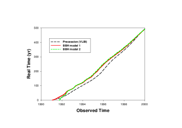
Figure 9: Rest frame time recovered from the precession fit (describing the trajectory of the VLBI component) and the BBH Models 1 and 2 (describing the optical variability) under the consistency constraints discussed in Sect. 4.4. The injection epoch $t_{\mathrm{inj}}=1991.05$ (for which $t_{\mathrm{rest}}=0$ is required by the precession fit) is reproduced by the BBH Model 1 and cannot be recovered from the BBH Model 2. The agreement between the precession fit and Model 1 ensures that the BBH scenario provides a single framework for describing simultaneously the observed trajectory and flux density changes of C7 and the observed variability of the optical emission of 3C 345

For the earliest epochs of the evolution of C7, Model 2 does not reproduce satisfactorily the separations of C7 from the core (Fig. 10) and the flux density changes (Fig. 11). The discrepancy between the fits by the precession model and Model 2 is particularly visible in the speed evolution obtained from the precession and BBH fits (Fig. 12). Model 1 is therefore a better counterpart to the precession fit described in Sect. 5.1.

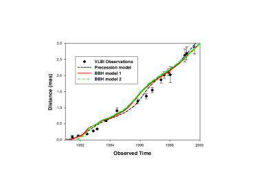
Figure 10: Evolution of the separation of the jet component C7 from the core. The fit by the precession model is consistent with the fit by BBH Model 1. BBH Model 2 fails to reproduce the earliest position measurements of C7.

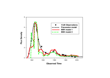
Figure 11: Radio flux density of C7 at 22 GHz. The fits by the precession model and BBH Model 1 are consistent. BBH Model 2 cannot reproduce the onset of the radio emission.

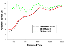
Figure 12: Apparent speed evolution of the jet component C7 recovered from the precession and BBH fits. The fit by BBH Model 1 is consistent with the fit by the precession, while BBH Model 2 cannot be reconciled with the precession fit at all.

Figure 13 compares the precession and the BBH Model 1 fits to the observed two-dimensional path of C7. The agreement between the fits is excellent. The two fits differ by less than 0.02 mas (Fig. 14). This deviation is caused by the orbital motion of the black hole ejecting the jet, which is not accounted for in the precession fit.

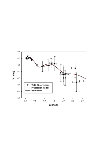
Figure 13: Two-dimensional path of C7. The precession fit and the fit by BBH Model 1 are presented.

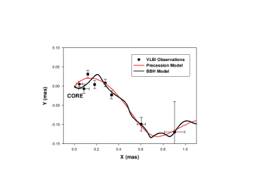
Figure 14: Two-dimensional path of C7 within 1 mas of the nucleus. The difference between the precession and BBH Model 1 fit is due to the orbital motion of the black hole ejecting the jet.

5.4 Optical light curve and orbital period

Fitting the optical light curve constrains the orbital period $T_{\mathrm{o}}$, orbital eccentricity and initial orbital phase $\phi_{\mathrm{o}}$ in the BBH system, under the conditions of consistency described in Sect. 5.3. The fit to the optical curve requires a nearly circular orbit ($e<0.1$), constrains uniquely the initial orbital phase

$$\phi_{\mathrm{o}}=125\degr$$

and produces a family of solutions for $T_{\mathrm{o}}$ depending on the value of $V_{\mathrm{A}}$. These solutions are presented in Table 5 for the same range of $V_{\mathrm{A}}$ as in Table 4. The fit to the optical light curve is shown in Fig. 15. It does not depend on the actual value of $T_{\mathrm{o}}$ because $T_{\mathrm{o}}V_{\mathrm{A}}^{-1}=const$, and thus the same shape of the lightcurve can be reproduced by a number of combinations of $V_{\mathrm{A}}$ and $T_{\mathrm{o}}$.

Table 5: Orbital period solutions for $V_{\mathrm{A}}=0.05\,c$–$0.15\,c$

Parameter	Value
$V_{\mathrm{a}}$ $[c]$	0.050	0.075	0.078	0.100	0.125	0.150
$T_{\mathrm{0}}$ $[{\mathrm{y}rs}]$	770	505	480	375	290	250

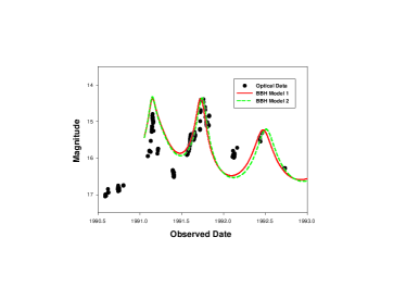
Figure 15: Optical variability in 3C 345 in 1990–93. Solid lines show the fits by the BBH model. Individual peaks result from the orbital motion in the BBH system.

5.5 Determination of the Alfvén speed

In order to reconcile the two families of $V_{\mathrm{A}}$-dependent solutions (the precession solutions in Table 4 and the orbital period solutions in Table 5), the value of the Alfvén speed must be constrained. The periodic changes of the position angle of component ejection plotted in Fig. 7 can be used for this purpose. The Alfvén wave perturbations, propagating at $V_{\mathrm{A}}\ll v_{\mathrm{c}}$ cannot account for such a short period. The observed period $P_{\mathrm{short}}\approx 9.5$ yr must therefore reflect perturbations of the magnetic field caused by the orbital motion in the BBH system. In this case, $T_{\mathrm{o}}=P_{\mathrm{short}}\delta_{\mathrm{c,0.5\,mas}}$, where $\delta_{\mathrm{c,0.5\,mas}}$ is the Doppler factor of the beam plasma measured at the same location (0.5 mas from the nucleus) at which the oscillations of the ejection angle are registered. The kinematic fit yields $\delta_{\mathrm{c,0.5\,mas}}=50$, which results in the orbital period $P_{\mathrm{o}}=480$ yr. The corresponding value of the Alfvén speed is then

$$V_{\mathrm{A}}=0.078\,c\,.$$

It should be noted that the Doppler factor $\delta_{\mathrm{c,0.5\,mas}}=50$ is similar to the Doppler factors implied by the observed statistics of superluminal motions near blazar cores (Jorstad et al. 2001a ).

5.6 Parameters of the binary system

With the Alfvén speed determined, the masses of the black holes can now be estimated from $T_{\mathrm{o}}$ and $T_{\mathrm{p}}$. Since the orbital separation $r_{\mathrm{o}}\propto(M_{1}+M_{2})^{1/3}$, a family of solutions can be produced that satisfy $T_{\mathrm{o}}=480$ yr, $T_{\mathrm{p}}=2570$ yr and reproduce the observed optical lightcurve of 3C 345 and radio properties of C7 (the shapes of the optical and radio lightcurves depend on the mass ratio $\mu_{1,2}=M_{1}/M_{2}$). The resulting solutions are presented in Table 6 for five selected values of $M_{1}$.

In order to identify an acceptable solution for the black hole masses, stability conditions of the accretion disk must be considered. The rotational timescale of a precessing accretion disk in a binary system is given by a characteristic period (Laskar & Robutel lr95 (1995))

$$T_{\mathrm{disk}}=\frac{4}{3}\left(\frac{M_{1}}{M_{2}}+1\right)\frac{T_{\mathrm{o}}^{2}}{T_{\mathrm{p}}}\,.$$

The disk in a BBH system will be stable over timescales comparable with the typical timescales of existence of a powerful radio source in AGN, $\tau_{\mathrm{agn}}\la 10^{8}$ yr, if two conditions are satisfied:

1.

$M_{1}\geq M_{2}$, where $M_{1}$ is the mass of the black hole surrounded by the accretion disk.

2.

$T_{\mathrm{disk}}\leq T_{\mathrm{o}}/2$

These conditions restrict the mass of the primary black hole to a range $7.1\times 10^{8}{\mathrm{M}}_{\sun}\leq M_{1}\leq 7.5\times 10^{8}{\mathrm{M}}_{\sun}$. The lower limit corresponds to $\mu_{1,2}=1$, and the upper limit corresponds to $P_{\mathrm{disk}}=P_{\mathrm{o}}/2=240$ yr. The acceptable range of $M_{1}$ is very narrow, and any value within this range can be adopted. Since $\mu_{1,2}$ does not change significantly over the acceptable range of $M_{1}$ ($\mu_{1,2}=1.02$ for $M_{1}=7.5\times 10^{8}{\mathrm{M}}_{\sun}$), $\mu_{1,2}=1$ can be adopted for the binary black hole mass solution, yielding

$$M_{1}=M_{2}=7.1\times 10^{8}{\mathrm{M}}_{\sun}$$

listed in Tables 2 and 6.

Table 6: Black hole mass solutions for $T_{\mathrm{o}}=480$ yr

Parameter	Value
$M_{1}$ $[10^{8}M_{\sun}]$	2.0	6.0	7.1	20.0	60.0
$M_{2}$ $[10^{8}M_{\sun}]$	4.0	6.6	7.1	12.3	23.1
$r_{\mathrm{o}}$ $[{\mathrm{p}c}]$	0.25	0.32	0.33	0.44	0.60
$T_{\mathrm{disk}}$ $[{\mathrm{y}rs}]$	179	229	239	314	430

Notes: $r_{\mathrm{o}}$ – orbital separation between the black holes, $T_{\mathrm{disk}}$ – characteristic rotational period of the accretion disk around the primary black hole.

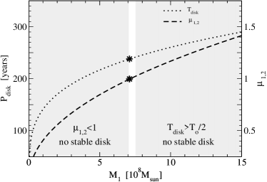
Figure 16: Range of acceptable solutions for the mass $M_{1}$ of the primary black hole in 3C 345. The acceptable solutions exist within the range $7.1\times 10^{8}{\mathrm{M}}_{\sun}\leq M_{1}\leq 7.5\times 10^{8}{\mathrm{M}}_{\sun}$. Asterisks mark the solution for $\mu_{\mathrm{1,2}}=1$, for which $M_{1}=M_{2}=7.1\times 10^{8}{\mathrm{M}}_{\sun}$. Shaded areas cover the values of $M_{1}$, $T_{\mathrm{o}}$ and $\mu_{1,2}$ for which the accretion disk cannot remain stable over the typical timescale of existence of a powerful radio source in AGN, $\tau_{\mathrm{agn}}\leq 10^{8}$ yr.

6 Discussion

The BBH model applied to the quasar 3C 345 ties together, within a single framework, the variability of the optical flux and the evolution of the superluminal feature C7 resulted from a powerful flare that occurred in 1991. The model reconstructs the physical conditions in the plasma ejected into the jet during the flare, and the dynamic properties of the binary system of supermassive black holes.

The binary black hole scenario was previously applied to 3C 345 by Caproni & Abraham (ca04 (2004)) who attributed variations of the ejection angle (similar to those plotted in Fig. 7) to precession of the accretion disk. This approach yielded an uncomfortably short precession period of $2.5\leq T_{\mathrm{p}}\leq 3.8$ yr, very high black hole masses ($M_{1}=4$–$5\times 10^{9}{\mathrm{M}}_{\sun}$, $M_{2}=3$–$4\times 10^{9}{\mathrm{M}}_{\sun}$), and extremely small orbital separation $r_{\mathrm{o}}=0.017$–$0.024$ pc, which is $\approx 100\,R_{\mathrm{G}}$ of the primary black hole. In such a tight binary, the effective accretion radius of the secondary, $r_{\mathrm{a}}=0.034$–$0.050$ pc, is larger than the orbital separation, and it is very difficult to maintain the accretion disk intact. Indeed, it can be shown (Ivanov, Igumenshchev & Novikov iin98 (1998)) that the mass loss rate $\dot{m}_{2}$ due to a shock that is formed after each passage of the secondary through the accretion disk may be very large, and for the BBH parameters of Caproni & Abraham (ca04 (2004)), it can reach $\dot{m}_{2}\approx\dot{M}_{1}(\sqrt{10}\,\alpha_{\star}^{4/5})^{-1}$, where $\dot{M}_{1}$ is the rate of accretion on the primary black hole and $\alpha_{\star}=\alpha/10^{-2}$ is the disc viscosity. For weak accretion rates or small disk viscosity, $\dot{m}_{2}$ can even become larger than $\dot{M}_{1}$, which would most likely lead to a subsequent destruction of the accretion disk.

Another argument against associating the ejection angle variability with the disk precession is presented by the observed long-term kinematic changes in the jet. The apparent accelerations plotted in Fig. 6 and the long-term trend present in the ejection angle changes plotted in Fig. 7 indicate the presence of a periodic process on timescales of $\sim 2000$ yr. This observed periodicity, though very difficult to establish, agrees well with the precession period recovered by fitting the BBH model to the trajectory and flux evolution of C7.

The trajectory of C7 (and indeed the trajectories of several other superluminal features monitored closely in the jet of 3C 345; Lobanov & Zensus lz96 (1996); L (96); LZ (99)) is clearly non-ballistic on timescales spanning almost 10 years in the observer’s frame (and more than 100 years in the comoving frame). This is a clear observational argument against a very short precession period in 3C 345. The model developed in this paper attributes non-ballistic trajectories of the jet features to Alfvén perturbations of the magnetic field, possibly modulated by the orbital motion in the system.

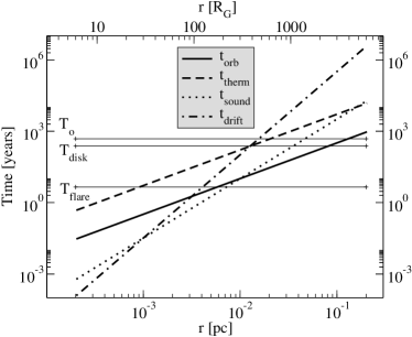
Figure 17: Characteristic timescales of disk activity in 3C 345, compared to the quasi-period of the nuclear flares and to the orbital and characteristic disk rotation periods). The disk thermal instability operates at $t\sim 4$ yr at distances of $\sim 20\,R_{\mathrm{G}}$. The mechanical (sound wave) instability reaches the same timescale at $\sim 200\,R_{\mathrm{G}}$, where it becomes comparable with the orbital and drift (accretion rate variations) timescales of the disk. A combination of these effects may cause the flare activity observed in 3C 345.

The sum of the black hole masses ($M_{1,2}=1.4\times 10^{9}{\mathrm{M}}_{\sun}$) estimated in our model agrees well with the mass $M_{\mathrm{bh}}=(4.0\pm 2.4)\pm 10^{9}{\mathrm{M}}_{\sun}$ obtained from measurements of nuclear opacity and magnetic field strength in 3C 345 (Lobanov 1998a ). Gu, Cao & Jiang (gcj01 (2001)) report a higher value of $M_{\mathrm{bh}}=7.6\times 10^{9}{\mathrm{M}}_{\sun}$ for 3C 345, from the properties of the broad line region. This estimate, however, depend strongly on the monochromatic luminosity ($M_{\mathrm{bh}}\propto L_{5100{\mathrm{\AA}}}^{2}$) for which the errors can be as large as 30% even for the nearby objects (Kaspi et al. kas+00 (2000)). This error could be even larger for weaker objects (3C 345 is about 100 times weaker in the optical than an average object from the sample of Kaspi et al. 2000), and overestimating $L_{5100{\mathrm{\AA}}}^{2}$ by only 50% would be bring the $M_{\mathrm{bh}}$ down to a value similar to the one derived in this paper.

Finally, let us consider the periodicity of the flares and component ejections in 3C 345. A $\sim 4$ yr period of the flaring activity is inferred from the observed variability of the radio nucleus (LZ (99)), and it is related with the ejections of superluminal features (see Fig. 3). Since this period is much shorter than $T_{\mathrm{p}}=2570$ yr, $T_{\mathrm{o}}=480$ yr and $T_{\mathrm{disk}}=240$ yr obtained in our model, there should be some other periodic process affecting the accretion disk on timescales of $\sim 4$ yr. Figure 17 shows four different characteristic disk timescales in 3C 345, for the black hole and disk parameters determined in Sect. 4. These timescales can be compared to the periodicity of the nuclear flares. It appears that several processes occurring in the disk at radial distances of 20–200$\,R_{\mathrm{G}}$ may have similar characteristic timescales. Thermal instability at $\sim 20\,R_{\mathrm{G}}$ and mechanical (sound wave) instability at $\sim 200\,R_{\mathrm{G}}$ will develop at timescales of $\sim 4$ yr. In addition to this, the orbital and drift (accretion rate variation) timescales approach $\sim 4$ yr at $\sim 200\,R_{\mathrm{G}}$. A combination of these effects can cause the observed flare activity.

Another possible explanation for the observed flares is an intermediate or stellar mass black hole or even a neutron star orbiting the primary black hole at $r_{\star}\sim 800-1200\,R_{\mathrm{G}}$ at a large angle with respect to the accretion disk plane. Close approaches to, or even passages through, the accretion disk should lead to formation of shock waves in the disk (Ivanov, Igumenshchev & Novikov iin98 (1998); Šubr & Karas sk99 (1999)), which in turn would cause an increase in the accretion rate resulting in a nuclear flare and injection of a dense plasma cloud into the jet.

The periodicity of the flares may also be caused by a turbulence in the jet. Formation of a turbulent layer close to the beam-jet boundary can enhance the pair creation rate in the beam, which would be observed as the appearance, and propagation, of a bright feature embedded in the flow.

7 Conclusions

The model developed in this paper explains the variability of the optical flux and the kinematic and emission properties of the feature C7 observed in the relativistic jet of 3C 345 after a strong nuclear flare. The dynamic properties of the system are described in the framework of the orbital motion in a binary system of supermassive black holes and the precession of an accretion disk around the primary black hole. The emission and physical properties of relativistic plasma produced during the flare are treated within the two-fluid approach postulating a highly relativistic $e^{\pm}$ beam propagating inside an $e^{-}p$ jet. The $e^{-}p$ jet transports a major fraction of the kinetic power associated with the outflow from the nucleus of 3C 345, stabilizes the $e^{\pm}$ beam against plasma instabilities and shields it from interaction with the external medium.

Determination of the properties of the jet and the binary system in 3C 345 is a difficult process involving two major steps. First, the precession characteristics of the accretion disk are determined by fitting the kinematic and flux density evolution of C7. This yields a precession period $T_{\mathrm{p}}=2570$ yr, which is in a good agreement with the periodicities inferred from the changes of kinematic properties of individual jet components and variations of the ejecting position angle in 3C 345.

In the second step, the orbital and physical properties of the binary system are recovered by fitting the observed optical variability. This yields an orbital period of $T_{\mathrm{p}}=480$. The consistency between the two fits is ensured by requiring the fit to the optical light curve to reproduce also the kinematic and flux density evolution of C7. The consistency argument constrains the properties of radio and optically emitting plasma, with $\Gamma_{\mathrm{min,opt}}=12$ and $\Gamma_{\mathrm{min,rad}}=4$.

After ensuring consistency between the two fits, they are combined in order to constrain the Alfvén speed $V_{\mathrm{A}}=0.078\,c$, and make it popsible to recover the physical properties of the system. In the last step, the conditions of disk stability are employed to determine the individual masses of the binary companions. This procedure yields $M_{1}=M_{2}=7.1\times 10^{8}{\mathrm{M}}_{\sun}$. Finally, the model offers an explanation for the observed 4-year quasi periodicity of nuclear flares in 3C 345. This quasi-periodicity arises naturally from the characteristic timescales of the accretion disk surrounding the primary black hole. The overall success that the model has in explaining a variety of the observational properties in 3C 345 argues in favor of this explanation.

References

- (1) Abraham, Z. & Carrara, E. A. 1998, ApJ, 496, 172
- (2) Abraham, Z. & Romero, G. E. 1999, A&A, 344, 61
- (3) Achatz, U. & Schlickeiser, R., 1993, A&A, 274, 165
- (4) Aller, M. F., Aller, H. D. & Hughes, P. A. 2003, ApJ, 586, 33
- (5) Angione, R. J., Moore, E. P., Roosen, R. G. & Sievers, J. 1981, AJ, 86, 653
- (6) Attridge, J. M., Roberts, D. H., & Wardle, J. F. C. 1999, ApJ, 518, 87
- (7) Bååth, L. B. Rogers, A. E. E., Inoue, M., et al. 1992, A&A, 257, 31
- (8) Babadzhanyants, M. K., & Belokon’, E. T. 1984, Astrophysics, 20, 461
- (9) Babadzhanyants, M. K., Belokon’, E. T. & Gamm, N. G. 1995, Astronomy Reports, 39, 393
- (10) Belokon, E. T. & Babadzhanyants, M. K. 1999, Astronomy Letters, 25, 781
- (11) Begelman, M. C., Blandford, R. D. & Rees, M. J. 1980, Nature, 287, 307
- (12) Biretta, J. A., Moore, R. L. & Cohen, M. H. 1986, ApJ, 308, 93
- (13) Biretta, J. A., Sparks, W. B. & Macchetto, F. 1999, ApJ, 520, 621
- (14) Blandford, R. D. & Rees, M. J. 1978, in Pittsburgh Conference on BL Lac Objects, ed. A. M. Wolfe (Pittsburgh: University of Pittsburgh), 328
- (15) Britzen, S., Roland, J., Laskar, J. et al. 2001, A&A, 374, 784
- (16) Caproni, A. & Abraham, Z. 2004, ApJ, 602, 625
- (17) Camenzind, M. & Krockenberger, M. 1992, A&A, 255, 59
- (18) Cohen, M. H. 1985, in Extragalactic Energetic Sources, ed. V. K. Kapahi (Bangalore: Indian Academy of Sciences), 1
- (19) Despringre, V. & Fraix-Burnet, D. 1997, A&A, 320, 26
- (20) Feretti, L., Comoretto, G., Giovannini, G., et al. 1993, ApJ, 408, 446
- (21) Gu, M., Cao, X. & Jiang, D. R. 2001, MNRAS, 1111
- (22) Hanasz, M. & Sol, H. 1996, A&A, 315, 355
- (23) Hewitt, A. & Burbidge, G. 1993, ApJS, 87, 451
- (24) Ivanov, P. B., Igumenshchev, I. V. & Novikov, I. D. 1998, ApJ, 507, 131
- (25) Ivanov, P. B., Papaloizou, J. C. B. & Polnarev, A. G. 1999, MNRAS, 307, 79
- (26) Jorstad S. G., Marscher A. P., Mattox J. R. et al. 2001, ApJ, 556, 738
- (27) Jorstad S. G., Marscher A. P., Mattox J. R. et al. 2001, ApJS, 134, 181
- (28) Kaastra, J. S. & Roos, N. 1992, A&A, 254, 96
- (29) Kaspi, S., Smith, P. S., Netzer et al. 2000, ApJ, 533, 631
- (30) Kidger, M. R. 1988, PASP, 100, 1248
- (31) Kidger, M. R. 1989, A&A, 226, 9
- (32) Kidger, M. R. & de Diego, J. A. 1990, A&A, 227, L25
- (33) Kinman, T. D., Lamla, E., Ciurla, T., Harlan, E., & Wirtanen, C. A. 1968, ApJ, 152, 357
- (34) Klare, J. 2003, PhD Thesis, University of Bonn, Germany
- (35) Kolgaard, R. I., Wardle, J. F. & Roberts, D. H. 1989, ApJ, 97, 1550
- (36) Königl, A. 1981, ApJ, 243, 700
- (37) Laing, R. & Bridle, A. H. 2002, MNRAS, 336, 1161
- (38) Laing, R. & Bridle, A. H. 2004, MNRAS, 348, 1459
- (39) Laskar, J. 1990, in “Méthodes Modernes de la Mécanique Céleste”, eds. D. Benest, C. Froeschlé, 89
- (40) Laskar J. & Robutel P. 1995, Celestial Mechanics, 62, 193
- (41) Lehto, H. J., & Valtonen, M. J. 1996, ApJ 460, 270
- (42) Leppänen, K. J., Zensus, J. A., & Diamond, P. J. 1995, AJ, 110, 2479
- L (96) Lobanov, A. P. 1996, PhD Thesis, NMIMT, Socorro, USA (L96)
- (44) Lobanov, A. P. 1998a, A&A, 330, 79
- (45) Lobanov, A. P. 1998b, A&AS, 133, 261
- (46) Lobanov, A. P., Carrara, E. & Zensus, J. A. 1997, Vistas in Astronomy, 41, 253
- (47) Lobanov, A. P. & Zensus, J. A. 1996, in ASP Conf. Ser. v. 100, Energy Transport in Radio Galaxies and Quasars, ed. P. E. Hardee, J. A. Zensus & A. H. Bridle (San Francisco: ASP), 124
- LZ (99) Lobanov, A. P. & Zensus, J. A. 1999, ApJ, 521, 509 (LZ99)
- (49) Lü, P. K. 1972, AJ, 77, 829
- (50) Makino, J. 1997, ApJ, 478, 58
- (51) Makino, J. & Ebisuzaki, T. 1996, ApJ, 465, 527
- (52) Marcowith, A., Henri, G. & Pelletier, G. 1995, MNRAS, 277, 681
- (53) Marcowith, A., Henri, G., & Renaud N. 1998, A&A, 331, L57
- (54) McGimsey, B. Q., Smith, A. G., Scott, R. L., et al. 1975, AJ, 80, 895
- (55) Pelletier, G., Sol, H. & Asseo, E., 1988, Phys. Rev. A 38, 2552
- (56) Pelletier, G. & Roland, J. 1989, A&A, 224, 24
- (57) Pelletier, G., Roland, J., 1990. In: “Parsec-Scale Jets”, eds. J. A. Zensus & T. J. Pearson, (Cambridge University Press: Cambridge), 323
- (58) Pelletier, G. & Sol, H. 1992, MNRAS, 254, 635
- (59) Pollock, J. T., Pica, A. J., Smith, A. G., et al. 1979, AJ, 84, 1658
- (60) Polnarev, A. G. & Rees, M. J. 1994, A&A, 283, 301
- (61) Rieger, F. M. & Mannheim, K. 2000, A&A, 359, 948
- (62) Roland J. & Hermsen W. 1995, A&A, 297, L9
- (63) Roland, J. & Hetem, A., 1996, in: Cygnus A: Study of a radio galaxy, eds. C. L. Carilli & D. E. Harris, (Cambridge University Press, Cambridge), 126
- (64) Roland, J., Peletier, G. & Muxlow, T. 1988, A&A, 207, 16
- (65) Roland J., Teyssier R. & Roos N. 1994, A&A, 290, 357
- (66) Roos, N., Kaastra, J. S. & Hummel, C. A. 1993, ApJ, 409, 130
- R (00) Ros, E., Zensus, J. A. & Lobanov, A. P. 2000, A&A, 354, 55 (R00)
- (68) Sillanpää, A., Haarala, S. & Valtonen, M. J. 1988, ApJ, 325, 628
- (69) Schramm, K.-J., Borgeest, U., Camenzind, M., et al. 1993, A&A, 278, 391
- (70) Skibo, J.G., Dermer, C.D. & Schlickeiser, R. 1997, ApJ, 483, 56
- (71) Smyth, M. J. & Wolstencroft, R. D. 1970, A&ASS, 8, 471
- (72) Sol H., Pelletier G. & Asseo E. 1989, MNRAS, 237, 411
- (73) Steffen, W., Zensus, J. A., Krichbaum, T. P., Witzel, A. & Qian, S. J. 1995, A&A, 302, 335
- (74) Šubr, L. & Karas, V. 1999, A&A 352, 452
- (75) Teräsranta, H., Tornikoski, M., Mujunen, A., et al. 1998, A&AS, 132, 305
- (76) Tingay, S. J., Jauncey, D. L., Reynolds, J. E., et al. 1998, AJ, 115, 960
- (77) Valtaoja, E., Teräsranta, H., Tornikoski, M. et al. 2000, ApJ, 531, 744
- (78) Vicente, L., Charlot, P. & Sol, H. 1996, A&A 312, 727
- (79) Vio, R., Cristiani, S., Lessi, O. & Salvadori, L. 1991, ApJ, 380, 351
- (80) Unwin, S. C., Cohen, M. H., Pearson, T. J., et al., 1983, ApJ, 271, 536
- (81) Unwin, S. C., Wehrle, A. E., Urry, C. M., et al., 1994, ApJ, 432, 103
- (82) Unwin, S. C., Wehrle, A. E., Lobanov, A .P., et al., 1997, ApJ, 480, 596
- (83) Waltman, E. B., Fiedler, R. L., Johnston, K. J., et al. 1991, ApJS, 77, 379
- (84) Webb, J. R., Smith, A. G., Leacock, R. J., et al. 1988, AJ, 95, 374
- (85) Zensus, J. A. 1997, ARA&A, 35, 607
- (86) Zensus, J. A., Krichbaum, T. P. & Lobanov, A. P. 1995, Proc. Natl. Acad. Sci. USA, 92, 11348
- (87) Zensus, J. A., Krichbaum, T. P. & Lobanov, A. P. 1996, Rev. Mod. Astron., 9, 241
- ZCU (95) Zensus, J. A., Cohen, M. H. & Unwin, S. C. 1995, ApJ, 443, 35 (ZCU95)
- (89) Zensus, J. A., Ros, E., Kellermann, K. I., Cohen, M. H., Vermeulen, R. C. & Kadler, M. 2002, AJ, 124, 662