Extreme Gravitational Lensing near Rotating Black Holes

Abstract

We describe a new approach to calculating photon trajectories and gravitational lensing effects in the strong gravitational field of the Kerr black hole. These techniques are applied to explore both the imaging and spectral properties of photons that perform multiple orbits of the central mass before escaping to infinity. Viewed at large inclinations, these higher order photons contribute $\sim 20\%$ of the total luminosity of the system for a Schwarzschild hole, whilst for an extreme Kerr black hole this fraction rises to $\sim 60\%$. In more realistic models these photons will be re-absorbed by the disc at large distances from the hole, but this returning radiation could provide a physical mechanism to resolve the discrepancy between the predicted and observed optical/UV colours in AGN. Conversely, at low inclinations, higher order images re-intercept the disc plane close to the black hole, so need not be absorbed by the disc if this is within the plunging region. These photons form a bright ring carrying approximately $10\%$ of the total disc luminosity for a Schwarzchild black hole. The spatial separation between the inner edge of the disc and the ring is similar to the size of the event horizon. This is resolvable for supermassive black holes with proposed X-ray interferometery missions such as MAXIM, so has the potential to provide an observational test of strong field gravity.

1 Introduction

Black holes are the ultimate test of strong gravity, spacetime so warped that not even light can escape. By definition they have no emission (apart from Hawking radiation), yet their immense gravitational potential energy can be tapped by any infalling material. This can power a luminous accretion flow where the emission has its origin close to the black hole event horizon, as is seen in many objects including Active Galactic Nuclei, Galactic black hole binaries, Ultra-Luminous X-ray Sources and Gamma Ray Bursts. Photons emitted in this region are subject to general relativistic effects such as light-bending, gravitational lensing and redshift, as well as special relativistic effects as the emitting material will be moving rapidly (e.g. Fabian et al. 2000). These are well-understood from a theoretical standpoint, so accreting objects provide a natural laboratory to test the properties of strong gravitational fields.

Calculations of the relativistic corrections to photon properties have been ongoing for nearly three decades, starting with the classic work of Cunningham (1975) who calculated the distortions expected on the spectrum of a geometrically thin, optically thick, Keplerian accretion disc orbiting a Kerr black hole. Interest in these calculations dramatically increased with the realisation that the accretion disc could emit line as well as continuum radiation. Iron K$\alpha$ fluorescence resulting from X-ray irradiation of the accretion disc can give a narrow feature, on which the relativistic distortions are much more easily measured than on the broad accretion disc continuum Fabian et al. (1989). Since then, several groups have developed numerical codes that are capable of determining these effects both for standard discs (Dovciak, Karas & Yaqoob, 2004) and alternative emission geometries (Bursa et al., 2004).

While the problem is well-defined, there are many technical and numerical issues which arise in calculating the effects of strong gravity. Lightbending can result in lensing which strongly amplifies the emission, so a very small area of the accretion flow can make a large contribution on the observed flux. Here we describe how to efficiently calculate the effects of strong lightbending, and illustrate the effectiveness of this approach by using the code to compute the most extreme lightbending possible, the higher order images and spectra of an accretion disc (Viergutz, 1993; Bao, Hadrava & Ostgaard, 1994; Cadez, Fanton & Calvani, 1998). The first order image is from photons from the underside of the disc which are bent back into the observers line of sight, while second order images are produced by photons from the upper side of the disc which complete a full orbit around the black hole before reaching the observer. Obviously such paths must cross the equatorial plane, so are likely to re-intercept the disc. For an optically thick disc then this returning radiation adds to the intrinsic disc emission, and can enhance the emissivity at small radii for extreme Kerr black holes though it has little effect for Schwarzchild (Cunningham, 1976; Laor, Netzer & Piran, 1990; Agol & Krolik, 2000).

Nonetheless, the first order image of the disc can dominate the flux at high inclinations if the optically thick disc has rather limited radial extent. Even if it does not, some of the higher order image flux can escape to the observer through the inner ’hole’ in the disc below the radius of the minimum stable orbit, assuming that the plunging region is optically thin (but see Reynolds & Begelman 1997). The fraction escaping through this inner ’hole’ is rather larger for Schwarzchild than for Kerr, as the size of the gap between the innermost stable orbit and horizon is larger for the non-spinning black hole. Obviously, such paths are exquisitely sensitive to the gravitational potential, being close to the true photon orbit point which is the (unstable) crossover between capture by the black hole, and escape to infinity. This makes them potentially an excellent test of strong gravity, and they could be observable in nearby luminous AGN with micro-arcsec imaging X-ray interferometers such as MAXIM (Gendreau et al. 2001).

Such instruments could also observe the spin of a nearby supermassive black hole simply from the size of the direct image (Fukue, 2003; Takahashi, 2004), assuming that the mass and distance are known. A disc down to the last stable orbit extends down to 6 $R_{g}$ in Schwarzchild but only 1.23 $R_{g}$ in extreme Kerr. Lightbending is stronger in Kerr than in Schwarzchild, but the apparent size of the ’hole’ in the disc still changes by a factor of $\sim 3$. This contrasts with the case where the accretion flow has emission down below the last stable orbit, where the size of the true black hole shadow is rather similar for both Schwarzchild and Kerr (Falcke, Melia, & Agol, 2000; Takahashi, 2004). Observations of the galactic black hole binaries support to the idea that there is a disc down to the minimum stable orbit in certain, fairly high luminosity spectral states (Ebisawa et al., 1993; Kubota et al., 1999; Gierliński & Done, 2004). However, at lower luminosities this is probably replaced by a more complex accretion flow which may have continuous energy release down to the horizon (Narayan & Yi, 1995; Agol & Krolik, 2000; Krolik & Hawley, 2002; Afshordi & Paczyński, 2003). While the stellar remnant black holes require nano-arcsecond imaging to resolve, nearby luminous AGN also should have a ’hole’ in the disc from the minimum stable orbit which is accessible to MAXIM.

The paper is split into two parts. In Section 2 we introduce the relevant theory necessary to perform efficient calculation of photon properties in strong gravity, including a review the properties of the effective potentials governing photon motion. In Section 3, we apply these techniques to examine the contribution of orbiting photons to the standard accretion disc solution through images of the inner region of the accretion flow, generation of fluorescent Iron K$\alpha$ line profiles and the relative roles played by the different types of photon paths. Readers not interested in technical details should go straight to Section 3.

2 Calculating Photon Paths in Strong Gravity

2.1 Null Geodesic Equations

Material in an accretion flow near to a black hole emits radiation, which is received by a (possibly distant) observer. These photons enable the observer to form an image of the flow, which in turn determines the measured spectral properties (Beckwith & Done, 2004). In the geometric optics approximation, the photons follow null geodesics, which in the Kerr metric (written in Boyer-Lindquist coordinates with $G=M=c=1$) are described by (Chandrasekhar, 1983):

$$\begin{split}p^{r}=\dot{r}=\rho^{-2}\sqrt{R_{\lambda,q}(r)}\\ p^{\theta}=\dot{\theta}=\rho^{-2}\sqrt{\Theta_{\lambda,q}(\theta)}\\ p^{\phi}=\dot{\phi}=\rho^{-2}\Delta^{-1}\left[2ar+\lambda\left(\rho^{2}-2r\right)\mathrm{cosec}^{2}\theta\right]\\ p^{t}=\dot{t}=\rho^{-2}\Delta^{-1}\left(\Sigma^{2}-2ar\lambda\right)\end{split}$$ (1)

where as usual $a$ is the angular momentum of the source (normalised to mass so that $a=1$ corresponds to the ’extremal’ case) and dotted quantities denote differentiation with respect to some affine parameter. We introduce the metric functions $\Delta=r^{2}-2r+a^{2}$, $\rho^{2}=r^{2}+a^{2}\cos^{2}\theta$, $\Sigma^{2}=\left(r^{2}+a^{2}\right)^{2}-a^{2}\Delta\sin^{2}\theta$ and the effective potentials (Viergutz 1993):

$$\begin{split}R_{\lambda,q}\left(r\right)=\left[\left(r^{2}+a^{2}\right)-a\lambda\right]^{2}-\Delta\left[q-\left(\lambda-a\right)^{2}\right]\\ \Theta_{\lambda,q}\left(\theta\right)=q+a^{2}\cos^{2}\theta-\lambda^{2}\mathrm{cot}^{2}\theta\end{split}$$ (2)

Here $\lambda,q$ are constants of motion which are related to the photons covariant angular and linear momenta (see Chandrasekhar 1983; de Felice & Preti 1999). The Kerr metric is both stationary and axisymmetric so the derived set of geodesic equations (1) are independent of both of the coordinates $t$ and $\phi$. The properties of a given geodesic path (specified by a $\lambda,q$ pair) are completely determined by the first two of these equations, which can be merged together and integrated to form a governing equation:

$$\begin{split}\pm\int^{r}{\frac{dr}{\sqrt{R_{\lambda,q}(r)}}}=\pm\int^{\theta}{\frac{d\theta}{\sqrt{\Theta_{\lambda,q}(\theta)}}}\end{split}$$ (3)

Consider the radial motion of the geodesic, described by the left-hand side of the above. We fix the ends of the radial trajectories at $r_{e}$ and $r_{o}$, which leads us to the general form for radial motion:

$$\begin{split}I^{s^{1}_{r},s^{2}_{r}}_{r,\lambda,q}\left(r_{e},r_{o}\right)=\pm\int^{r_{o}}_{r_{e}}{\frac{dr}{\sqrt{R_{\lambda,q}(r)}}}\\ =s^{1}_{r}\left[\int^{r_{t}}_{r_{e}}{\frac{dr}{\sqrt{R_{\lambda,q}(r)}}}+s^{2}_{r}\int^{r_{t}}_{r_{o}}{\frac{dr}{\sqrt{R_{\lambda,q}(r)}}}\right]\end{split}$$ (4)

Here, we have denoted the radial turning point (either perihelion or aphelion) of the path motion by $r_{t}$ and $s^{1,2}_{r}$ can take the values $-1,+1$ dependent on the nature of the path. From the discussion of Wilkins (1972), there are no bound null geodesics that terminate above the horizon, implying that at most there can be one radial turning point along the geodesic path. There are therefore three types of radial motion that we must consider:

1. From $r_{e}$ to $r_{o}$ with no radial turning point encountered, implying either $\left(s^{1}_{r}=+1,s^{2}_{r}=-1\right)$ if $r_{e}<r_{o}$ or $\left(s^{1}_{r}=-1,s^{2}_{r}=-1\right)$ if $r_{e}>r_{o}$.

2. From $r_{e}$ inwards to perihelion at $r_{t}$, then outwards to $r_{o}$, implying that $\left(s^{1}_{r}=-1,s^{2}_{r}=+1\right)$ for $r_{t}<r_{e}$, $r_{t}<r_{o}$.

3. From $r_{e}$ outwards to aphelion at $r_{t}$, then inwards to $r_{o}$, implying that $\left(s^{1}_{r}=+1,s^{2}_{r}=+1\right)$ for $r_{t}>r_{e}$, $r_{t}>r_{o}$.

For the latitudinal motion we can, in general, have an arbitrary number of turning points occur along the path (unlike in the radial case). This requires a more complex expression to describe the contribution of the latitudinal motion. We introduce the variable $m=\cos\theta$:

$$\begin{split}I^{s^{1}_{m},s^{2}_{m},n_{m}}_{m,\lambda,q}\left(m_{e},m_{o}\right)=\pm\int^{m_{o}}_{m_{e}}{\frac{dm}{\sqrt{M_{\lambda,q}(m)}}}\\ =s^{1}_{m}\left[\int^{m_{+}}_{m_{e}}{\frac{dm}{\sqrt{M_{\lambda,q}(m)}}}+s^{2}_{m}\int^{m_{+}}_{m_{o}}{\frac{dm}{\sqrt{M_{\lambda,q}(m)}}}\right]\\ +\left[2n_{m}-s^{1}_{m}s^{2}_{m}\left(1+s^{2}_{m}\right)\right]\int^{m_{+}}_{m_{-}}{\frac{dm}{\sqrt{M_{\lambda,q}(m)}}}\end{split}$$ (5)

The effective potential now takes the form $M_{\lambda,q}(m)=q+m^{2}\left(a^{2}-\lambda^{2}-q\right)-a^{2}m^{4}$. In the above, $m_{+,-}$ denote the locations of the latitudinal turning points determined by solution of $M_{\lambda,q}(m)=0$ (Rauch & Blandford, 1994), whilst $n_{m}$ denotes the number of such turning points through which the path passes and $s^{1,2}_{m}$ can take the values $-1,+1$. Specifically, the case of $s^{1}_{m}$ is described by two possibilities:

1. If $m_{+}=-m_{-}$, then $s^{1}_{m}=+1,-1$ dependent on whether the path is initially directed towards the ’north’ or ’south’ poles of the hole respectively.

2. If $m_{+}\neq-m_{-}$, then $s^{1}_{m}$ is in the direction of the closest of $m_{+,-}$ to $m_{e}$

The sign of $s^{2}_{m}$ is determined by the number of turning points, $n_{m}$ through which the geodesic passes, $s^{2}_{m}=-1^{n_{m}}$.

Geodesic paths are therefore described by:

$$I^{s^{1}_{r},s^{2}_{r}}_{r,\lambda,q}\left(r_{e},r_{o}\right)-I^{s^{1}_{m},s^{2}_{m},n_{m}}_{m,\lambda,q}\left(m_{e},m_{o}\right)=0$$ (6)

This can be solved analytically in terms of elliptic functions, which is much more efficient than numerical solutions. Rauch & Blandford (1994) tabulate these functions to determine the observed coordinate latitude, $\theta_{obs}$ for photons with momenta $\left(\lambda,q\right)$ emitted from a given radius and latitude which arrive at the observers’ radial coordinate. Alternatively, Agol (1997); Cadez, Fanton & Calvani (1998) fix one end of the radial path at infinity with some inclination and the coordinates at which the other end crosses the equatorial plane. An additional method, due to Viergutz (1993) fixes the ends of the photon paths at the required coordinates, and a minimisation technique is applied to determine valid $\left(\lambda,q\right)$ pairs for a given number of orbits of the black hole.

Our approach combines aspects of those described by Rauch & Blandford (1994) and Viergutz (1993). We invert the reformulated governing equation to obtain the observed co-ordinate latitude of the geodesic, using the technique described by Rauch & Blandford (1994):

$$\begin{split}\int^{m_{+}}_{m_{o}}{\frac{dm}{\sqrt{M_{\lambda,q}(m)}}}=s^{1}_{m}s^{2}_{m}I^{s^{1}_{r},s^{2}_{r}}_{r,\lambda,q}\left(r_{e},r_{o}\right)\\ -s^{2}_{m}\int^{m_{+}}_{m_{e}}{\frac{dm}{\sqrt{M_{\lambda,q}(m)}}}\\ -s^{1}_{m}s^{2}_{m}\left[2n_{m}-s^{1}_{m}s^{2}_{m}\left(1+s^{2}_{m}\right)\right]\int^{m_{+}}_{m_{-}}{\frac{dm}{\sqrt{M_{\lambda,q}(m)}}}\end{split}$$ (7)

We apply the properties of the effective potentials described by Viergutz (1993) to dramatically reduce the scale of the calculation by analytically restricting the range of $\lambda$ and $q$ to those which can escape to infinity. Then we search this range for those paths which contribute to a given image order at the required observed inclination. These geodesics are then projected to form an image of the system on the observers sky, which is then used to determined the measured flux (described in Beckwith & Done 2004). The code therefore allows the fast calculation of geodesics linking any two points in the spacetime that make a specified number orbits of the black hole.

2.2 The Zeroes of the Effective Potentials

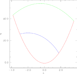
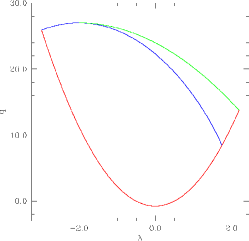
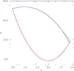
Figure 1: Boundary curves on the $(\lambda,q)$-plane for an extreme ($a=1$) Kerr black hole with $r_{o}=\infty$, $\theta_{e}=\pi/2$ and $\theta_{o}=30^{\circ}$. The graph of $q_{m,a}\left(\lambda\right)$ is shown by the red curve, $q_{r,a}\left(\lambda\right)$ by the green and $q_{c}\left(r_{c}\right),\lambda_{c}\left(r_{c}\right)$ by the blue. On the left-hand panel, the emitter is located at $r_{e}=6r_{g}$, such that $r_{e}>r^{(-)}_{ph}$ and hence the valid region is bounded by $q_{r,a}\left(\lambda\right)$ from above and $q_{m,a}\left(\lambda\right)$ from below, whilst the $q_{c}\left(r_{c}\right),\lambda_{c}\left(r_{c}\right)$ describes the line below which a photon directed radially inward is inevitably captured by the hole. In the central panel, the emitter is now located at $r_{e}=3r_{g}$, such that $r^{(-)}_{ph}\leq r_{e}\leq r^{(-)}_{ph}$. The parameter space is again bounded by $q_{m,a}\left(\lambda\right)$ from below, however in this case, the upper limit is given by $q_{c}\left(r_{c}\right),\lambda_{c}\left(r_{c}\right)$ for $\lambda\leq\lambda_{c}\left(r_{e}\right)$ and by $q_{r,a}\left(\lambda\right)$ otherwise. Finally, we see that for $r_{e}=2r_{g}$ (right-hand panel), these boundaries still apply, even though the graph of $q_{r,a}\left(\lambda\right)$ is now concave (true for all $r\leq 2r_{g}$).

To obtain solutions of the reformulated governing equation (6), we turn to the tables of elliptic integrals provided by Rauch & Blandford (1994), as modified by Agol (1997). These tables, when combined with appropriate numerical techniques allow us, in principle, to determine the geodesics that link an arbitrary emitter, $\left(r_{e},m_{e}\right)$ and observer, $\left(r_{o},m_{o}\right)$.

In practice, however, this calculation is far from trivial. By specifying the locations of the emitter and receiver, we have placed definite restrictions on the values of the angular momentum parameters, $(\lambda,q)$ for which geodesic motion between these two locations is even possible. The geodesic motion is dependent on the square root of the two effective potentials, $R_{\lambda,q}(r)$, $M_{\lambda,q}(m)$, which requires that these functions remain positive definite at all points along the path. If, at any point on the geodesic, this requirement is broken, then a potential barrier is necessarily formed and no such motion is possible. Viergutz (1993) has shown that these requirements can be expressed in terms of the interplay of a set of algebraic functions, which we consider further here. Note that the application of these functions enables us to provide tight limits on the region of parameter space which must be considered in the calculation and hence hugely reduce the scale of the calculation.

We begin by introducing:

$$\underline{r}=\min\left(r_{e},r_{o}\right);\;\;\overline{r}=\max\left(r_{e},r_{o}\right)$$

$$\underline{m}=\min\left(\left|m_{e}\right|,\left|m_{o}\right|\right);\;\;\overline{m}=\max\left(\left|m_{e}\right|,\left|m_{o}\right|\right)$$

The condition that no potential barrier exists between the emitter and observer can be re-expressed mathematically as:

$$R_{\lambda,q}\left(\underline{r}\leq r\leq\overline{r}\right)\geq 0;\;\;M_{\lambda,q}\left(\underline{m}\leq\left|m\right|\leq\overline{m}\right)\geq 0$$ (8)

Since the effective potentials are linear in $q$, we can express these requirements as:

$$q\leq q_{r,a}\left(\lambda\right);\;\;q\geq q_{m,a}\left(\lambda\right)$$ (9)

Here:

$$\begin{split}q_{r,a}\left(\lambda\right)=\frac{\left[r^{2}+a\left(a-\lambda\right)\right]^{2}}{\Delta}+\left(\lambda-a\right)^{2}\\ q_{m,a}\left(\lambda\right)=\frac{m^{2}}{1-m^{2}}\lambda^{2}-a^{2}m^{2}\end{split}$$ (10)

Physically, these curves correspond to the locus of points on the $\left(\lambda,q\right)$ plane for which the given co-ordinate, $\left(r,m\right)$ is a zero of the associated effective potential. For the latitudinal motion, it is found that there are two cases that we must consider (taking $\underline{m}$ as the pericentre of the latidunal motion and similarly $\overline{m}$ is the apocentre):

$$q\geq\begin{cases}q_{\underline{m},a}\left(\lambda\right)&\left|\lambda\right|<a\sqrt{1-\underline{m}^{2}}\sqrt{1-\overline{m}^{2}}\\ q_{\overline{m},a}\left(\lambda\right)&\left|\lambda\right|\geq a\sqrt{1-\underline{m}^{2}}\sqrt{1-\overline{m}^{2}}\end{cases}$$ (11)

The description of the radial motion is more complex, due to the existence of the unstable photon orbits Chandrasekhar (1983). These orbits are described by the existence of a further set of zeroes of the radial effective potential, $R_{\lambda,q}(r)=0$ that is subject to the additional constraint $\partial_{r}R_{\lambda,q}\left(r\right)=0$. These conditions yield a pair of parametric equations describing a critical curve on the $\left(\lambda,q\right)$ plane, which define the apparent angular size of the black hole:

$$\begin{split}\lambda_{c}=\frac{1}{a\left(r_{c}-1\right)}\left(r^{2}_{c}-a^{2}-r_{c}\Delta_{c}\right)\\ q_{c}=\frac{r^{3}_{c}}{a^{2}\left(r_{c}-1\right)^{2}}\left[4\Delta_{c}-r_{c}\left(r_{c}-1\right)^{2}\right]\end{split}$$ (12)

The range of values of $r_{c}$ is given by considering the solutions of $4a^{2}=r_{c}\left(r_{c}-3\right)^{2}$ (corresponding to the radii of unstable photon orbits, either direct or retrograde, in the equatorial plane). Following Chandrasekhar (1983), we denote these radii by $r^{(+)}_{ph}$ and $r^{(-)}_{ph}$ and so $r^{(+)}_{ph}\leq r_{c}\leq r^{(-)}_{ph}$.

The second complication to this discussion stems from Wilkins (1972). Specifically, for any particle, orbits with $E^{2}>\delta^{2}$ (where $E^{2}$ denotes particle energy; $\delta^{2}=1,0$ particle mass), are unbound, whilst orbits with $E^{2}<\delta^{2}$ are bound. Since photons are massless, this implies that the only bound orbits are those with negative $E^{2}$ (and so must terminate behind the horizon), whilst all others must be unbound (except for a set of unstable, circular orbits). We cannot therefore (unlike in the previous discussion) consider trajectories with $\underline{r}$ as pericentre and $\overline{r}$ as apocentre.

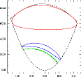
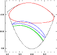
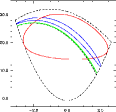
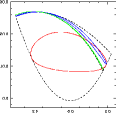
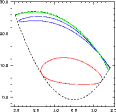
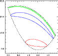
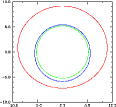
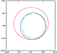
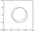
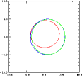
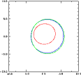
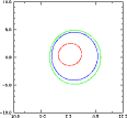
Figure 2: Closed geodesic loops on the $(\lambda,q)$-plane (top row) and their projection onto the observers sky (the $\alpha,\beta$ plane, bottom row) for an extreme ($a=1$) Kerr black hole with $r_{o}=\infty$, $\theta_{e}=\pi/2$ and $\theta_{o}=30^{\circ}$. Geodesics with $N=0$ are shown as red loops, those with $N=1$ as blue loops and $N=2$ as green loops. Also shown for references on the $(\lambda,q)$-plane representation are the parameter space boundaries (black dashed lines). From left to right, the each panel has $r_{e}=8,6,4,3,2,1r_{g}$. Note the change in the relative locations of the loops as the emitter moves inwards - for $r_{e}=8r_{g}$, the loops for each image order are completely detached. However, as the emitter moves in to $6r_{g}$, the $N=0,1$ loops overlap and by the time the emitter reaches $4r_{g}$, the $N=0$ loop overlaps both the $N=1$ and $N=2$ loop. At $3r_{g}$, the $N=0$ loop again crosses the $N=1,2$ loops, however in this case the $N=1$ and $N=2$ loops now touch. Moving the emitter inward to $2r_{g}$, the $N=0$ loop detaches itself and moves inside the $N=1,2$ loops, which cross. Moving the emitter still further inward, to just above $r_{+}$, we now see that $N=1,2$ loops have detached, with the $N=1$ loop now occurring between the $N=0,2$ loops.

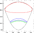
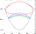
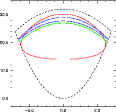
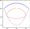
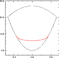
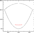
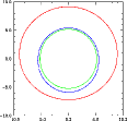
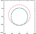
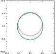
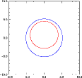
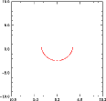
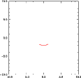
Figure 3: As in Figure 5 for a Schwarzschild ($a=0$) black hole, with (from left to right) $r_{e}=8,6,4,3,2.5,2r_{g}$. The loops display a qualitatively similar behaviour to that described in the $a=1$ case. We note that the restoration of spherical symmetry to the system (due to the absence of rotation) has removed the asymmetry of the loops on both planes and hence changed the points of overlap of the loops with respect to the $a=1$ case. For $r_{e}\leq 3r_{g}$, there are no photons with $N=2$ that propagate to infinity, furthermore for $r_{e}<3r_{g}$, there are no $N=1$ photons that can propagate to infinity either. More importantly, for $r_{e}<3r_{g}$ a distant observer is unable to form a complete (that is $\phi=0\to 2\pi$) image of the ring even using direct ($N=0$) photons.

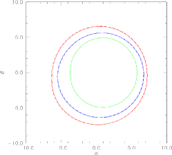
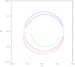
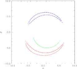
Figure 4: Two emitting rings around an extreme Kerr black hole located at $r_{e}=6r_{g}$ and $\theta^{a}_{e}=149^{\circ}$ (solid lines), $\theta^{b}_{e}=151^{\circ}$ (dashed lines) with the colour coding as in Figure 5. The observer is located at radial infinity with polar coordinate $\theta_{o}=25^{\circ}$ (left panel), $\theta_{o}=30^{\circ}$ (centre panel) and $\theta_{o}=35^{\circ}$ (right panel). In the left panel, $\left|\theta_{o}\right|<\left|\theta^{a,b}_{e}\right|$, producing circular images of the emitting rings. In the centre panel, we now have that $\left|\theta^{a}_{e}\right|<\left|\theta_{o}\right|<\left|\theta^{b}_{e}\right|$ and the image of the $\theta^{a}_{e}$ ring has now separated such that the zeroth and second order images appear from the south pole of the hole, whilst the first order image appears from behind the north pole. Finally, in the right-hand panel, we have that $\left|\theta_{o}\right|>\left|\theta^{a,b}_{e}\right|$ and so images of both $\theta^{a,b}_{e}$ follow this behaviour.

For our purposes, three particular cases describing the behaviour of the $q_{r,a}(\lambda)$ curve are of interest. To illustrate these, we consider an extreme Kerr ($a=1$) hole, with the observer located at radial infinity and an inclination of $\theta_{o}=30^{\circ}$. We locate the emitter in the equatorial plane and begin by considering the case $r^{(-)}_{ph}\leq\underline{r}$ (Figure 1, left panel). Here, the region of the angular momentum $(\lambda,q)$ plane for which no potential barrier is formed between the emitter and observer is bounded from below by $q_{m,a}(\lambda)$, as described by equation 11. The upper limit of this region is provided by $q_{\underline{r},a}(\lambda)$ and it can be shown that, independent of the locations of the emitter and observer, these curves are concave and convex functions of $\lambda$, respectively. This indicates that we can provide limits on the allowed range of $\lambda$ via:

$$\begin{split}\lambda_{+,-}\left(\overline{m},\underline{r},a\right)=\\ \frac{2a\underline{r}\left(1-\overline{m}^{2}\right)\pm\sqrt{\underline{\Delta}}\sqrt{1-\overline{m}^{2}}\left(\underline{r}^{2}+\overline{m}^{2}a^{2}\right)}{\underline{\Delta}-a^{2}\left(1-\overline{m}^{2}\right)}\end{split}$$ (13)

The apparent angular size of the black hole is defined by the parametric curve $q_{c}\left(r_{c}\right),\lambda_{c}\left(r_{c}\right)$. Hence, photons whose angular momentum falls under this curve and are directed initially inwards towards the hole from $\underline{r}$ are inevitably captured. For $r^{(-)}_{ph}\leq\underline{r}$, this critical curve intersects the graph of $q_{m,a}(\lambda)$ at some $\lambda^{+,-}_{c}$ (the exact intersection being determined numerically) and so inwardly directed photons with $\lambda^{-}_{c}\leq\lambda\leq\lambda^{+}_{c}$, $q_{m,a}(\lambda)\leq q\leq q_{c}(r_{c})$, where $r_{c}$ is determined by inversion of $\lambda=\lambda_{c}(r_{c})$, can be completely excluded from the calculation.

We now move the location of the emitter inwards such that $r^{(+)}_{ph}\leq\underline{r}\leq r^{(-)}_{ph}\leq\overline{r}$ (Figure 1, centre panel). We have that the valid region of the angular momentum plane is bounded from below by $q_{m,a}(\lambda)$, as before. The behaviour of the upper bound to the angular momentum plane is, however, quite different. In this case, since $r^{(+)}_{ph}\leq\underline{r}\leq r^{(-)}_{ph}$, there exists some $r^{*}_{c}=\underline{r}$, which is associated with a $(\lambda^{*}_{c},q^{*}_{c})$ pair, through equations (12). For $\lambda\leq\lambda^{*}_{c}$, we therefore have that the upper limit of the angular momentum plane is given by the critical curve and hence the lower limit on $\lambda$ is determined by $\lambda^{+}_{c}$. Similarly, above $\lambda^{*}_{c}$, the upper limit on the plane is given, as in the previous case, by $q_{\underline{r},a}(\lambda)$ and so the upper limit on $\lambda$ is given by $\lambda_{+}(\overline{m},\underline{r},a)$. Note that, for $\lambda\leq\lambda^{*}_{c}$ there are no photons that are emitted on radially inbound geodesics that reach the observer, whilst for $\lambda>\lambda^{*}_{c}$, only those initially ingoing photons with values of $q$ above the critical curve can reach the observer. Finally, we note that for the emitter located at $\underline{r}\leq 2r_{g}$ (Figure fig:2.2.1, right-hand panel), the graph of $q_{r,a}(\lambda)$ is now convex. However, the relationship between the various curves remains unchanged from that described in the previous case and the angular momentum plane remains bound.

2.3 Structure & Properties of Geodesics Loops

We begin by considering solutions to the ’governing’ equation for a simple system where the emitter is located in the equatorial plane of an extreme Kerr ($a=1$) hole ($\theta_{e}=\pi/2$) and takes the form of an infinitesimal ring located at radius $r_{e}$. For such an infinitesimal ring, the flux is undefined (since the ring subtends zero solid angle on the observers sky) and so we concentrate our attention on the behaviour of the solutions on the $\left(\lambda,q\right)$ and $\left(\alpha,\beta\right)$ planes (Figure 2). To minimise the impact of gravitational lensing, we locate the observer at radial infinity and $\theta_{o}=30^{\circ}$ (as previously).

Initially, we locate the ring at $r_{e}=8r_{g}$ (Figure 2, panel a) and catalogue the complete set of geodesics of zeroth ($N=0$), first ($N=1$) and second ($N=2$) order. Each of these geodesic orders form a closed loop on both the $\left(\lambda,q\right)$ and $\left(\alpha,\beta\right)$ planes. We note that the projections on both planes are asymmetric about the line $\lambda,\alpha=0$ due to the breaking of spherical symmetry by the black hole spin and also (for the emitter located at $8r_{g}$) that the loops for each individual image order are completely detached. We now move the emitter inwards to $r_{e}=6r_{g}$ (Figure 2, panel b), which causes the loops associated with the zeroth and first order images to overlap. The solutions to the geodesic equations are therefore multivalued at these points in $\left(\lambda,q\right)$ space, breaking the statement by Cunningham (1975) that there are two geodesics linking a point on the accretion disc to an observer for each value of the redshift parameter, $g$, which (for the Keplerian disc considered by Cunningham), corresponds to two geodesics at each valid point in $\lambda$ space. If we now move the emitter inwards to $r_{e}=4r_{g}$ (Figure 2, panel c), we now see that the loops associated with the zeroth order geodesic now overlaps with both the first order loop and the second order loop.

We now move the emitter further inwards, so that $r^{(+)}_{ph}\leq r_{e}=3r_{g}<r^{(-)}_{ph}$ (Figure 2, panel d). Here, the zeroth order loop still overlaps the first and second order loops, however, in this case the first and second order loops now touch. Moving the emitter inwards still further to $r_{e}=2r_{g}$ (Figure 2, panel e), the zeroth order loop now detaches itself from the first and second order loops and moves inside these loops on the $\left(\alpha,\beta\right)$ plane projection. The apparent angular size of the zeroth order loop, as measured by the distant observer, is now smaller than that of the first and second order loops, which has important consequences for the calculation of the emergent flux, as we shall shortly see. Finally, we move the emitter down to $r_{e}-r_{g}=10^{-6}$ (Figure 2, panel f), the location of $r_{+}$ in Boyer-Lindquist coordinates (however, this is not the case in terms of proper distance, see Bardeen, Press & Teukolsky 1972). All of the loops are again detached, however, in comparison to the case where $r_{e}=8r_{g}$, the ordering of these loops is now reversed on the $\left(\alpha,\beta\right)$ plane, with the second order now subtending the greatest angular size of the observers sky.

We now replace the central extreme Kerr black hole with a Schwarzschild ($a=0$) black hole and repeat the preceding calculation. From Figure 3, we see that the behaviour of the solutions on the two planes is qualitatively similar to that of the extreme Kerr case as we move the emitter from $8r_{g}$ down to $4r_{g}$. However, in this case we note that the loops are now symmetric about the line $\lambda,\alpha=0$ due to the absence of rotation in the system and that this results in the quantitative locations of the overlap to change. Note that we can understand the existence of these overlaps by considering the meaning of the projection of these loops on the $\left(\lambda,q\right)$ plane. Recall that, for given $\left(\lambda,q\right)$ pair, there exists a set of roots $\left(r_{i},m_{i}\right)$ of the effective potentials $R_{\lambda,q}\left(r\right)$, $M_{\lambda,q}\left(m\right)$. Whether or not the geodesic path passes through selected members of these sets of roots depends on the initial direction taken by the geodesic, described by the $s_{r},s_{m}$ parameters in equation 6 and hence different geodesic paths can be described by a single $\left(\lambda,q\right)$ pair.

Consider now the behaviour of these loops as we move the emitter to $r_{e}=3r_{g}$ for the Schwarzschild hole (Figure 3, panel d). Here, we find that the zeroth and first order loops are now detached, but in this case the second order loop does not exist. Moving the emitter in further to $2.5r_{g}$ (Figure 3, panel e), we find that not only does the first order loop disappears, but the zeroth order loop is no longer closed! Finally, if we move the emitter to $r_{e}-2r_{g}=10^{-6}$ (Figure 3, panel f), then we find that we are only able to image a small line segment from the ring. To understand this behaviour, we turn to the discussion given by Chandrasekhar (1983) regarding the ’cone of avoidance’, describing the cone generated the photons that pass through the unstable circular orbits located at $3r_{g}$. We let $\psi$ denote the half-angle of the cone (directed inward at large distances from the hole) and it can then be shown that:

$$\tan\psi=\frac{1}{r/3-1}\sqrt{\frac{r/2-1}{r/6+1}}$$ (14)

We therefore see that for $r\leq 3r_{g}$, $\psi\leq\pi/2$, which implies that below $3r_{g}$, the apparent angular size of the black hole is greater than that of the distant stars. This shows that the black hole obscures part of the region $\phi=0\to 2\pi$ for a distant observer when the emitter is located below $r=3r_{g}$, which implies that the dynamics of the accretion flow in this region are extremely difficult to directly measure.

2.4 General Emission Geometries

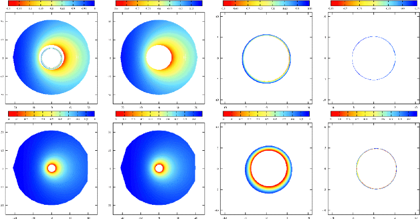
Figure 5: The contribution of orbiting photons (higher order images) to a distant observers image of a geometrically thin, optically thick, Keplerian accretion disc around Schwazschild (top row) and extreme Kerr (bottom row) black holes. In both cases the observer is located at radial infinity with $\theta_{o}=15^{\circ}$, the disc extends from the marginally stable orbit ($6r_{g}$ for Schwarzschild, $1r_{g}$ for extreme Kerr) to $20r_{g}$ and the images are coloured by the associated value of the redshift parameter, $g=E_{o}/E_{e}$. From left to right, the panels show the contributions from (a) all image orders ($N=0\cdots 2$), (b) the direct ($N=0$) image, (c) the first order ($N=1$) image and (d) the second order ($N=2$) image. Note that in the Schwarzschild case whilst the orbiting photons are not obscured from the observer by the accretion disc, the total flux (integrated area) measured by the observer from the photons is negligible. Additionally, for the Kerr case, the increased radial extent of the disc completely obscures the contribution of the photons.

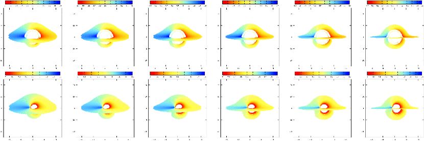
Figure 6: As in Figure 5 showing the contribution of photons with $N=0\cdots 2$. From left to right, the panels are for $\theta_{o}=75.0^{\circ}\cdots 87.5^{\circ}$ in steps of $2.5^{\circ}$. As the inclination of the system increases, the contribution from photons emitted from the near side of the accretion disc directly to the observer is suppressed, reducing the obscuration of the higher order images by the disc as measured by the observer. The total area subtended by the unobscured first order ($N=1$) image increases independently of this effect, due to lensing of photons that are emitted from the underside of the far side of the accretion disc, relative to the observer. In the case of the Schwarzschild hole (top row), we note that the (total) area of the second order image remains approximately constant with inclination. For the extreme Kerr hole (bottom row), photons forming the second order image are completely absorbed by the disc, removing their contribution from the overall image received by the observer. Additionally, in contrast to the Schwarzschild case, the images are asymmetric about the $\alpha=0$ axis due to the effect of black hole spin, particularly noticeable for the higher order cases. For the most extreme inclination, the total area subtended by the first order image is on the same order as that from the direct image.

In the standard picture of accretion onto a massive compact object, the emitting material is located in the equatorial plane in what is assumed to be a geometrically thin structure. As such, gravitational lensing effects only come into play for high inclination systems ($\theta_{o}>60^{\circ}$). However, if one wishes to consider emission from a non-equatorial geometry (the case of a geometrically thick, optically thin accretion flow, for example), then gravitational lensing effects can have important consequences even for low inclination observers. As an example, consider again two infinitesimal rings, located at $r_{e}=6r_{g}$, with polar coordinates $\theta^{a}_{e}=149^{\circ}$ and $\theta^{b}_{e}=151^{\circ}$. We again locate the observer at radial infinity and initially take $\theta_{o}=25^{\circ}$ such that $\left|\theta_{o}\right|<\left|\theta^{a,b}_{e}\right|$ (Figure 4 left panel). The two rings form are mapped continuously onto the $\left(\alpha,\beta\right)$ plane for each individual image order in a similar fashion to those considered previously. We now move the latitudinal coordinate of the observer to $\theta_{o}=30^{\circ}$, such that $\left|\theta^{a}_{e}\right|<\left|\theta_{o}\right|<\left|\theta^{b}_{e}\right|$ (Figure 4 centre panel). The image of the lower ring, $\theta^{b}_{e}$ is again mapped continuously onto the $\left(\alpha,\beta\right)$ plane for each individual image order, as would be expected as it’s relationship to the latitudinal coordinate of the observer has remained unchanged. This is not true however of the image of the upper ring, $\theta^{a}_{e}$, which is now mapped discontinuously onto the $\left(\alpha,\beta\right)$ plane, with the even image orders (zeroth and second) appearing from the southern hemisphere of the hole and the odd image orders (first) appearing from the northern hemisphere. It is therefore clear that, in order to generate a complete picture of the physical properties of such a system, we must include the contribution of the higher orders to the calculation. Finally, we again move the observer in the latitudinal direction to $\theta_{o}=35^{\circ}$, such that $\left|\theta_{o}\right|>\left|\theta^{a,b}_{e}\right|$ (Figure 4 right panel). Now the images of both rings are mapped discontinuously onto the $\left(\alpha,\beta\right)$ plane, which serves to further emphasise the importance of the inclusion of the higher order images in the calculation.

3 Results & Discussion

3.1 Images of Thin Keplerian Accretion Discs

The contribution of higher order images to the observed flux is dependent both on the location of the observer and the angular momentum of the hole itself, together with the assumed geometry and emissivity of the accretion flow. For an optically thick accretion disc then any photons which re-intersect the disc after emission will be either absorbed (and then re-emitted) or reflected by the material. Figure 5 shows the contributions of both the direct ($N=0$)and higher order ($N=1,2$) images of a geometrically thin disc extending from $r_{ms}$ to $20r_{g}$, viewed at $\theta_{o}=15^{\circ}$ for both Schwarzschild and maximal Kerr black holes. The principle effect of black hole spin for the accretion disk dynamics is to move the location of the marginally-stable orbit, $r_{ms}$ and hence the location of the inner edge of the accretion disc. In the case of the Schwarzschild hole, the inner edge of the accretion disc is located at $6r_{g}$, above the radius of the unstable photon orbits ($3r_{g}$) so higher order image photons which cross the equatorial plane below $6r_{g}$ are not absorbed by the disc and may be able to freely propagate to the observer. This contrasts with the extreme Kerr hole behaviour, where the accretion disc extends down to $1r_{g}$, completely obscuring the allowed radial range of the unstable photon orbits ($1r_{g}\leq r_{c}\leq 4r_{g}$, though mostly $3r_{g}$ for the polar orbits which dominate the low inclination image) and hence the contribution of the higher order photons is completely obscured by the accretion disc.

Figure 6 shows the same systems viewed at a range of large inclination angles, $\theta_{o}=75^{\circ}-87.5^{\circ}$. As in the previous discussion for the Schwarzschild hole, the inner edge of the accretion disc is located above the location of the photon orbits and hence the majority of the orbiting photons are able to propagate freely to the observer. However, photons in the first order image of the far side of the disc now have paths which pass rather closer to the hole than at lower inclination, so the importance of lensing is increased, strongly amplifying this part of the image. Most of these photons cross the equatorial plane at $r\geq 20r_{g}$, so can be seen in our simulation, but would be obscured by a more physically realistic disc which is not entirely flat and has outer edge $r\gg 20r_{g}$. These photons instead would illuminate a large region of the underside of the disc as the direct image of the disc, adding to its intrinsic emission. By contrast, the area on the sky of the second order image remains approximately constant with increasing inclination, reflecting the sensitivity (i.e. instability) of the two-loop photon orbits.

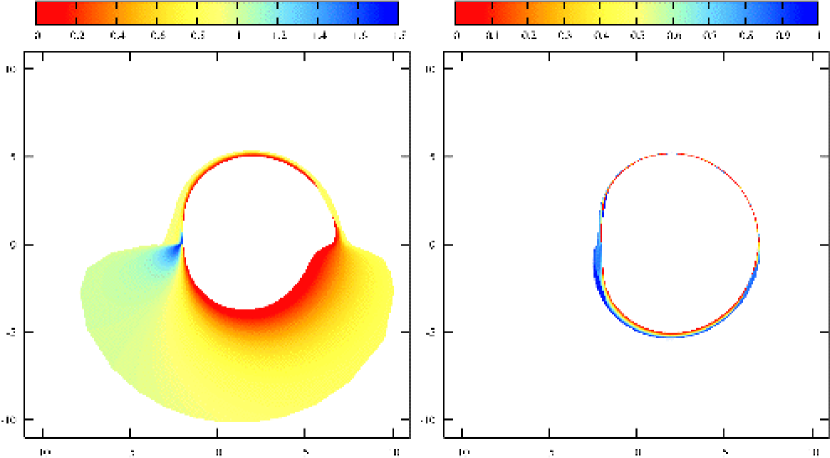
Figure 7: Unobscured $N=1$ (left-hand panel) and $N=2$ (right-hand panel) images of a thin, Keplerian accretion disc around an extreme Kerr black hole, with the disc extending from $r_{ms}$ to $20r_{g}$. The observer is located at radial infinity with an inclination of $\theta_{o}=87.5^{\circ}$. The images are highly asymmetric, indicating the strong coupling of these photons to the bacl hole spin

The high inclination extreme Kerr images are shown in Figure 6, bottom row. The disc itself blocks all the higher orbit images close to the black hole, similar to the $\theta_{o}=15^{\circ}$ case. Part of the first order image where the geodesic crosses the equatorial plane at $r\geq 20r_{g}$ can be seen, and this fraction increases with increasing inclination of the observer. Indeed, for the highest inclination system considered in this work, the apparent angular size of the first order image is approximately equivalent to that subtended by the direct image. By contrast to the Schwarzschild case, we note that the images of the extreme Kerr system are strongly asymmetric about the horizontal axis due to the effect of the black hole spin, with the degree of this asymmetry increasing with the inclination of the observer. This asymmetry is most pronounced for the (unobscured) first and second order images generated from the highest inclination system (see Figure 7). Here, the effect of the range of radii for orbiting photons can be seen most clearly in the second order image. The image is offset from zero as the ones on the left are the photons which are emitted from the side of the disc approaching the observer, so go with the spin of the black hole and orbit at $r_{g}$, while photons on the right are the retrograde ones at $4r_{g}$. The hole in the inner disc is symmetric at $r_{g}$, so it (just) obscures all the prograde photons and easily obscures the retrograde ones. A small decrease in spin (e.g. to a=0.998, the equilibrium spin for thin disc accretion) increases $r_{ms}$ to $1.23$, while the photon orbits span $1.07-3.998r_{g}$, so a small part of the prograde higher order image can be seen. The fraction of higher order photons which can escape through the ’hole’ increases with increasing spin until $a\lesssim 0.65$ Bardeen, Press & Teukolsky (1972), where the photon orbits are all within $r_{ms}$.

3.2 Spectral Properties of Higher Order Images

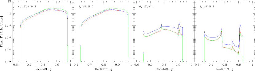
Figure 8: Relativistic line profiles generated from images (Figure 5, top row) of a geometrically thin, Keplerian accretion disc around a Schwarzschild $(a=0)$ black hole. The observer is located at $\theta_{o}=15^{\circ}$ and the disc extends from $r_{ms}$ to $20r_{g}$. All profiles are normalised such that they contain one photon and are unsmoothed. From left to right, the panels show the contributions from (a) photons with $N=0\cdots 2$, (b) $N=0$, (c) $N=1$, (d) $N=2$. In all cases a $\epsilon(r_{e})\propto r^{-3}_{e}$ radial emissivity has been applied to the line profile. We consider three different types of angular component (i) $f(\mu_{e})\propto\mathrm{cons.}$ (red lines), (ii) $f(\mu_{e})\propto\mu^{-1}_{e}$ (green lines) and (iii) $f(\mu_{e})\propto(1+2.06\mu_{e})$ (blue lines). We display the lines generated from the direct image (red line), first order (blue lines), second order (green lines) and the combined line profile (black line) using a standard $\varepsilon(r_{e})\propto r_{e}^{-3}$. the principle effect of the higher order images is to boost the overall flux in the system by $\sim 4\%$, whilst leaving the overall shape of the line approximately unchanged.

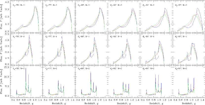
Figure 9: The contribution of orbiting photons (higher order images) to the Iron K$\alpha$ line profiles for a geometrically thin, Keplerian accretion disc around a Schwarzschild black hole. In all cases, the inner edge of the accretion disc is located at the innermost stable orbit, which occurs at $6r_{g}$ and the outer edge of the disc is located at $20r_{g}$. The observer is located at radial infinity with inclination (from left to right) $\theta_{o}=75^{\circ}\cdots 87.5^{\circ}$ in $2.5^{\circ}$ steps. All profiles are normalised to the apparent area on the observers sky and are unsmoothed. The line profiles are generated by photons in (a) the zeroth order (direct) image (top row), (b) the first order image (middle row) and (c) the second order image (bottom row). Obscuration by the disc is ignored. In all cases a $\epsilon(r_{e})\propto r^{-3}_{e}$ radial emissivity has been applied to the line profile. We consider three different types of angular component (i) $f(\mu_{e})\propto\mathrm{cons.}$ (red lines), (ii) $f(\mu_{e})\propto\mu^{-1}_{e}$ (green lines) and (iii) $f(\mu_{e})\propto(1+2.06\mu_{e})$ (blue lines). Line profiles generated by the zeroth order photons have the standard skewed, double peaked structure. Those generated by the first order photons have a similar structure, whilst those from the second order photons are far more complex. As the observer moves towards higher inclinations, gravitational lensing effects become apparent in the line profile generated from zeroth order photons. There is a corresponding increase in the complexity of the profile generated from the first order photons. Note however, that the structure of the profile generated from the second order photons remains approximately constant with increasing inclination.

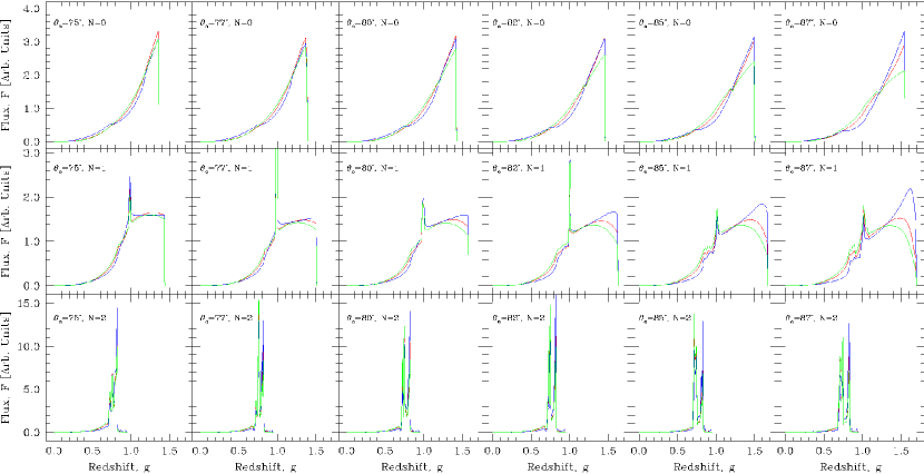
Figure 10: As in Figure 11 for accretion discs around an extreme Kerr black hole. By contrast to the Schwarzschild case, the lines extend down to lower energies due to the reduced separation between the inner edge of the disc (at the marginally stable orbit) and the black hole event horizon. Additionally, the line due to the first order photons extends to higher energies than that due to the zeroth order photons, with the upper edge of the line occuring at $g\approx 1.8$ in the most extreme case.. Both the first and second order line profiles have significantly increased structure compared to the zeroth order profile. The shape of the zeroth and second order line profiles remain approximately constant with increasing inclination. However, the internal structure of the first order profile shows a distinctive change, with the fraction of radiation in the blue wing of the profile exhibiting a marked increase compared to that in the red wing as the observer moves towards the equatorial plane.

To understand how the astrophysical properties of the accretion flow couple to the gravitational field of the black hole, we generate relativstically smeared line profiles as described in Beckwith & Done (2004). For clarity, we briefly recap this method here. We consider an intrisically narrow emission line with rest energy, $E_{e}$, for which the flux distribution measured by a distant observer at an energy $E_{o}$ is given by:

$$F_{o}\left(E_{o}\right)=\frac{1}{D_{o}^{2}}\int\int g^{4}\varepsilon\left(r_{e},\mu_{e}\right)\delta\left(E_{o}-gE_{int}\right)d\alpha d\beta$$ (15)

Here, $\varepsilon\left(r_{e},\mu_{e}\right)$ is the local emissivity of the accretion disc, which we take to have the form $\varepsilon\left(r_{e},\mu_{e}\right)=\epsilon\left(r_{e}\right)f\left(\mu_{e}\right)$, where $\mu_{e}$ describes the initial direction of the photon relative to the local z-axis of the emitting materlal. The flux at each redshift in each image order is then calculated directly from the area subtended on the observers sky, together with the intrinsic disc emissivity (both radial and angular). This gives the transfer function for monochromatic flux, so the observed emission is the convolution of this with the intrinsic disc spectrum. In the case of intrinsically monochromatic radiation, e.g. the iron K$\alpha$ fluorescence line which can be produced by X-ray illumination of cool, optically thick gas, then this transfer function directly gives the expected line profile. Photons produced by this emission process in regions close to the black hole enable us to examine the properties of the multiple orbit photons considered in the preceding section from a spectroscopic perspective.

To generate the line profiles, we apply a radial emissivity of the form $\epsilon(r_{e})\propto r^{-3}_{e}$ (consistent with gravitational energy release within the disc, Zycki, Done & Smith 1999) and consider three possible angular emissivity laws: (i) $f(\mu_{e})\propto\mathrm{cons.}$, corresponding to an optically thick disc (red lines); (ii) $f(\mu_{e})\propto\mu^{-1}_{e}$, corresponding to an optically thin, limb brightened disc (blue lines) (Matt, Perola & Stella, 1993) and (iii) $f(\mu_{e})\propto(1+2.06\mu_{e})$ corresponding to an optically thick, limb darkened disc (green lines) (Laor, Netzer & Piran, 1990). Figure 8 shows the line profiles generated for the low inclination Schwarzschild disc discussed in the preceding section. Whilst in the case of the extreme Kerr black hole (Figure 5, bottom row), all orbiting photons returned to the inner region of the disc, for the Schwarzschild hole (Figure 5, top row) these photons cross the equatorial plane below $r_{ms}$ and can freely propagate to the observer (although see Reynolds & Begelman 1997). Examination of their spectral properties shows that these photons play a limited role in forming the overall spectral shape measured by a distant observer, which is completely dominated by the contribution from the direct image.

Figure 9 shows the line profiles generated for a Schwarzschild hole, with the accretion disc now viewed at high inclination (ignoring the effect of obscuration). For the direct image, limb darkening boosts the effects of gravitational lensing, enhancing the flux from the far side of the hole. This is because these photons are strongly bent, i.e. are emitted from a lower inclination angle than that at which they are observed, so a limb darkening law means that the flux here is higher (Beckwith & Done, 2004). The doppler shifts are rather small for this material, so this lensing enhances the flux in the middle of the line. Since the line profiles are normalised to unity, this means that the blue wing is less dominant.

The first order spectra are shown in Figure 9, middle row. The transfer functions mostly retain the characteristic double peaked and skewed shape, and again the principle effect of the different angular emissivities is to alter the balance between the blue wing and lensed middle of the line. However, there is some new behaviour for the limb brightened emissivity. This has the largest change in emissivity with angle, and this combined with the exquisite sensitivity of lensed paths means that this picks out only a small area on the disc, leading to a discrete feature in the spectrum. These profiles also show enhancement of the extreme red wing of the line, as the photons which orbit generally are emitted from the very innermost radii of the disc.

The discrete features are completely dominant for all emissivities at second order (Figure 9, bottom row). These are images of the top of the disc where the photons have orbited the black hole, so the paths are even more sensitive to small changes than first order. Thus the profiles are significantly more complex in structure, being dominanted by lensing. There are blue and red features at the extreme ends of the line profile which are picking out the maximum projected velocity of the innermost radii of the disc. These have the standard blue peak enhancement. However, the two strong features redward of this are a pair of lensed features, from the near and far side of the disc.

Figure 10 shows the line profiles generated for the extreme Kerr hole at high inclinations, again ignoring the effect of obscuration. For the direct image (Figure 10, top row), the lines exhibit the characteristic triangular shape previously reported by (e.g) Laor (1991), with the variation in angular emissivity acting to alter the balance between the different regions of the line on a $\sim 5\%$ level. The lines associated with the first order image (Figure 10, middle row) exhibit a marked difference in comparison to those associated with the Schwarzschild black hole. In general, they are broader that those associated with the direct image and resemble a skewed Gaussian combined with a narrow line (due to caustic formation) at $g\approx 1.0$. Here the principle effect of changes in the angular emissivity is to alter the height of the blue wing, relative to the rest of the line. Again, the line profiles associated with the second order image (Figure 10, bottom row) are completely dominated by discrete features, as in the Schwarzschild case.

3.3 Image Luminosities

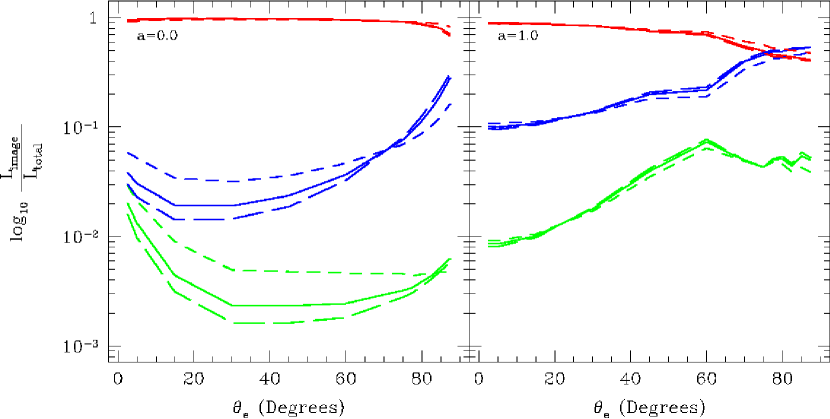
Figure 11: Variation of (unobscured, integrated) luminosity associated with each image as a fraction of the total luminosity of the system with inclination for a thin, Keplerian accretion disc around a Schwarzschild black hole (left panel) and extreme Kerr (right panel). In both cases, the disc extends from $r_{ms}$ to $20r_{g}$ and the observer is located at radial infinity. We show the contributions from (a) the direct image (red lines), (b) the first order image (blue lines) and (c) the second order image (green lines). In all cases, we have applied a $\epsilon(r_{e})\propto r^{-3}_{e}$ radial emissivity and have considered angular emissivities of the form (i) $f(\mu_{e})\propto\mathrm{cons.}$ (solid lines), (ii) $f(\mu_{e})\propto\mu^{-1}_{e}$ (short dashed lines) and (iii) $f(\mu_{e})\propto(1+2.06\mu_{e})$ (long dashed lines). In the case of the Schwarzschild hole, the contribution from the higher order images is $\leq 20\%$ of the total luminosity, even at high inclinations. However, in the case of the extreme Kerr black hole, at inclinations of $\geq 75^{\circ}$, the first order image can dominate the luminosity of the system, due to the formation of caustics within the image.

To understand the relative roles played by each (unobscured) image order, we consider the variation of the luminosity of each image as a fraction of the total luminosity of the system as a function of inclination, again for both Schwarzschild and extreme Kerr black holes (Figure 11). These luminosities are generated from the integral in redshift space of the line profiles considered in the preceding section and hence we consider systems with identical properties to those previously discussed. In the case of the Schwarzschild hole, we see that, for inclinations $<80^{\circ}$, the first order image can be regarded as a $\leq 10\%$ correction to the emergent flux from the system. For inclinations $\geq 80^{\circ}$, this image contains $~{}10-20\%$ of the emergent flux, i.e. even at these high inclinations, the first order image can still be regarded as a correction to the direct image. For the second order image, we see that it plays a $\leq 1\%$ role independent of inclination. Third and higher order images will have correspondingly smaller fluxes, so can safely be neglected.

There is a larger fraction of flux in the higher order images for the Kerr black hole. At low inclinations, the first and second order images contain $~{}10\%$ and $~{}1\%$ of the total flux, respectively. The variation of the luminosity fraction for the three image orders displays an approximately power law like behaviour for inclinations $\leq 60^{\circ}$, where a distinct break occurs, due to the appearance of a caustic in the first order image, whose luminosity is therefore significantly enhanced. It is at this point that the peak luminosity of the second order image occurs, which here is on the level of $~{}10\%$, approximately an order of magnitude higher than in the Schwarzschild case. Remarkably, for inclinations $>75^{\circ}$, the luminosity of the first order image produced by the optically thick discs is greater than that produced by the direct image.

However, most of the higher image order flux is expected to reintercept the disc plane, and hence be absorbed and reradiated. This is especially the case for realistic discs around an extreme Kerr black hole, where the whole of the equatorial plane is covered by the disc from $r_{g}$ to large radii. However, for Schwarzchild, the existance of a central ’hole’ means that the flux from higher order images can escape. A realistic disc around a Scharwzchild black hole when viewed face on has $~{}10\%$ of its flux in a higher order image ring (dropping to $\sim 7\%$ for a more extended disk ranging from $r_{ms}\to 400r_{g}$). Essentially, a spatial resolution equivalent to $2r_{g}$ is required to resolve these features, which for typical nearby Active Galactic Nuclei corresponds to an angular resolution of $~{}0.01$ microarcseconds. This is obviously extremely technically difficult, but is feasible for an X-ray interferometer imaging supermassive black holes in nearby galaxies (Gendreau et al., 2001).

4 Conclusions

Photons orbiting a black hole encounter the strongest possible gravitational fields compatible with still escaping to the observer. Thus these higher order null geodesics provide the best test of Einsteins gravity in the strong field limit. We have developed a new strong gravity code capable of describing these paths, and calculate them for a geometrically thin, optically thick (standard) disc in both Schwarzchild and Kerr metrics. These higher order image paths must cross the equatorial plane, so are absorbed where this is filled by the optically thick disc. As has long been known, the major amplification effects of gravitational lensing are for the first order paths from the far side of the underneath of the disc viewed at high inclination i.e. photons initially emitted downwards on the far side of the black hole, which are bent by gravity up above the disc plane. Most of these paths will re-intersect the disc unless it has very limited outer radial extent. While such discs may exist (Reynolds et al., 2004), it seems far more likely that these photons would be absorbed by material in the equatorial plane. However, there is some fraction of the higher order images where the light paths are so strongly bent that they re-intersect the equatorial plane very close to the photon orbit radius. By definition, this is below the minimum stable orbit for particles, so the standard disc cannot exist at this point. Instead, for a stress-free inner boundary condition, the disc material plunges rapidly though this region, so there is much less absorbing material in the equatorial plane. This material may be optically thick at high mass accretion rates (Reynolds & Begelman, 1997), but this depends on whether the flow in the plunging region in smooth or clumpy. Hence higher order photons which cross the plane below $6r_{g}$ need not be reabsorbed by the disc. We show that these observable higher order photons can carry 10% of the flux for a face on disc. Edge on discs reduce the expected observable flux as only about half of the orbiting photon ring can be seen through the gap below $r_{ms}$, while the rest re-intercepts the disc at $r\gg r_{ms}$.

The situation is less favourable in the Kerr geometry as photons now orbit at a range of radii depending on how their angular momemtum is aligned with the spin of the black hole. Photons going against the spin will orbit at radii which are larger than that of the minimum stable orbit of the disc, so should be absorbed rather than escaping through the inner ’hole’ in the disc (provided $a\gtrsim 0.65$). Thus for Kerr black holes, even though there is a greater fraction of photons in the higher order images, we expect that these are less observable due to the overlap between the photon and particle orbits. Also, even though there is still a gap between the last stable particle orbit and the aligned photon orbits, this gap is much smaller than in Schwarzchild, both in terms of radial coordinate and in terms of impact parameter on the sky. For a=0.998, the equilibrium spin for thin disc accretion, $r_{ms}=1.23r_{g}$ while the $r_{ph}^{(-)}=1.07$, so $\Delta r=0.16$. Since the photons orbit in slightly stronger gravity, their paths are more distorted, so the difference in their impact parameter at infinity is slightly less than the difference in radial coordinate. Thus the higher order images round a rapidly spinning black hole are much more difficult to spatially resolve from the direct image of the disc, and carry less flux than Schwarzchild as only a fraction re-intersect the plane below $r_{ms}$.

Thus the best chance of observing these higher order photon paths from a standard accretion disc is with a face-on Schwarzchild black hole. X-ray interferometry could potentially directly resolve such scales for supermassive black holes in nearby galaxies, and such missions are being seriously proposed (MAXIM: Gendreau et al. 2001). Even if the plunging region is optically thick, direct imaging with resolution $\leq 2r_{g}$ will clearly show the black hole spin from the apparent size of the ’hole’ in the center of the disc. The radial coordinate of the innermost stable orbit in an equilibrium spin Kerr metric is a factor of $\sim 3$ smaller than for Schwarzchild, which translates to a change in apparent size at infinity of the ’hole’ diameter from $\sim 5r_{g}$ (a=0.998) to $\sim 14r_{g}$ (a=0). This is important as recent papers have emphasised that the true size of the shadow of the event horizon (in effect the impact parameter of the orbiting photons, given fairly accurately by our second order image) is rather similar in both Schwarzchild and Kerr (Falcke, Melia, & Agol, 2000; Fukue, 2003; Takahashi, 2004). This is true, but different to the size of the ’hole’ defined by the innermost stable orbit of the disc. For continuous energy release down to the event horizon, the ’hole’ in the image of the accretion flow is set by the true shadow size, but for accretion flows where the energy is only released from stable particle orbits (the disc, as opposed to the plunging region) then the innermost stable orbit sets the size scale. Whether the energy release can be continuous across $r_{ms}$ is currently a matter of active research (Krolik & Hawley, 2002). However, there is clear observational evidence for an innermost stable orbit in the disc dominanted spectra of galactic black hole binaries (Ebisawa et al., 1993; Kubota et al., 1999; Gierliński & Done, 2004), so it seems likely that the accretion flow can take the standard thin disc form assumed here.

The spectral signatures of these photons only become apparent for high-inclination systems, where they carry between $\sim 20\%$ (Schwarzschild) and $\sim 60\%$ (extreme Kerr) of the total luminosity of the system. However, in a realistic system, the disc extends out to many thousands of gravitational radii from the black hole and so these photons return to the disc before reaching the observer. Far from the central black hole, the effect of the returning radiation is comparable to the gravitational potential energy of the material and so these photons can play an important role in shaping the properties of the disc here. In particular, reprocessing of this returning radiation at large distances from the hole will potentially provide a physical mechanism to flatten (at large radii) the $r^{-3/4}$ temperature profile of a planar accretion disc irradiated by a central source, which could help to resolve the conflict between the predicted and observed optical/UV colours in Active Galactic Nuclei (Koratkar & Blaes, 1999).

The code used to calculate these results is an extension of that of Beckwith & Done (2004). The new aspect described here is a set of analytic constraints on the possible photon trajectories which vastly reduce the scale of the calculation. This, combined with the use of the analytic integrals (elliptic functions) for the photon paths, has the result that the calculation of a photon trajectory linking two points (the emitter and observer, Viergutz 1993) can be performed by a simple minimisation, capable of being calulated to almost arbitrary accuracy on a standard desktop pc on time scales of a few minutes. This technique allows us to include the contribution of orbiting photons in the calculations without loss of resolution. The code is also flexible enough to be adapted to any accretion flow, and a future paper will consider the contribution of the higher order images in an optically thin, geometrically thick flow.

References

- Agol (1997) Agol E., 1997, PhDT, Univ. California, Santa Barbara.
- Agol & Krolik (2000) Agol E., Krolik J. H., 2000, ApJ, 528, 161
- Afshordi & Paczyński (2003) Afshordi N., Paczyński B., 2003, ApJ, 592, 354
- Bao, Hadrava & Ostgaard (1994) Bao G., Hadrava P., Ostgaard E., 1994, ApJ, 435, 55
- Bardeen, Press & Teukolsky (1972) Bardeen J. M., Press W. H., Teukolsky S. A., 1972, ApJ, 178, 347
- Beckwith & Done (2004) Beckwith K., Done C., 2004, MNRAS, 352, 353
- Bursa et al. (2004) Bursa M., Abramowicz M. A., Karas V., Kluzniak W., 2004, astro, astro-ph/0406586
- Cadez, Fanton & Calvani (1998) Cadez A., Fanton C., Calvani M., 1998, NewA, 3, 647
- Chandrasekhar (1983) Chandrasekhar S., 1983, mtbh.book,
- Cunningham (1975) Cunningham C. T., 1975, ApJ, 202, 788
- Cunningham (1976) Cunningham C., 1976, ApJ, 208, 534
- de Felice & Preti (1999) de Felice F., Preti G., 1999, CQGra, 16, 2929
- Dovciak, Karas & Yaqoob (2004) Dovčiak M., Karas V., Yaqoob T., 2004, ApJS, 153, 205
- Ebisawa et al. (1993) Ebisawa K., Makino F., Mitsuda K., Belloni T., Cowley A. P., Schmidtke P. C., Treves A., 1993, ApJ, 403, 684
- Fabian et al. (1989) Fabian A. C., Rees M. J., Stella L., White N. E., 1989, MNRAS, 238, 729
- Fabian et al. (2000) Fabian A. C., Iwasawa K., Reynolds C. S., Young A. J., 2000, PASP, 112, 1145
- Falcke, Melia, & Agol (2000) Falcke H., Melia F., Agol E., 2000, ApJ, 528, L13
- Fanton et al. (1998) Fanton C., Calvani M., de Felice F., Cadez A., 1997, PASJ, 49, 159
- Fukue (2003) Fukue J., 2003, PASJ, 55, 155
- Gendreau et al. (2001) Gendreau K. C., White N., Owens S., Cash W., Shipley A., Joy M., 2001, fomi.conf, 11
- Gierliński & Done (2004) Gierliński M., Done C., 2004, MNRAS, 347, 885
- Hollywood & Melia (1997) Hollywood J. M., Melia F., 1997, ApJS, 112, 423
- Koratkar & Blaes (1999) Koratkar A., Blaes O., 1999, PASP, 111, 1
- Kubota et al. (1999) Kubota A., Marshall F., Makishima K., Dotani T., Ueda Y., Negoro H., 1999, AN, 320, 353
- Krolik & Hawley (2002) Krolik J. H., Hawley J. F., 2002, ApJ, 573, 754
- Laor (1991) Laor A., 1991, ApJ, 376, 90
- Laor, Netzer & Piran (1990) Laor A., Netzer H., Piran T., 1990, MNRAS, 242, 560
- Matt, Perola & Stella (1993) Matt G., Perola G. C., Stella L., 1993, A&A, 267, 643
- Misner, Thorne and Wheeler (1973) Misner C. W., Thorne K. S., Wheeler J. A., 1973, grav.book,
- Narayan & Yi (1995) Narayan R., Yi I., 1995, ApJ, 452, 710
- Wilms et al. (2001) Wilms J., Reynolds C. S., Begelman M. C., Reeves J., Molendi S., Staubert R., Kendziorra E., 2001, MNRAS, 328, L27
- Rauch & Blandford (1994) Rauch K. P., Blandford R. D., 1994, ApJ, 421, 46
- Reynolds & Begelman (1997) Reynolds C. S., Begelman M. C., 1997, ApJ, 488, 109
- Reynolds et al. (2004) Reynolds C. S., Wilms J., Begelman M. C., Staubert R., Kendziorra E., 2004, MNRAS, 349, 1153
- Takahashi (2004) Takahashi R., 2004, ApJ, 611, 996
- Viergutz (1993) Viergutz S. U., 1993, A&A, 272, 355
- Wilkins (1972) Wilkins D. C., 1972, PhRvD, 5, 814
- Zycki, Done & Smith (1999) Zycki P. T., Done C., Smith D. A., 1999, MNRAS, 305, 231