The Bicoherence as a Diagnostic for Models of High Frequency QPOs

Abstract

We discuss the use of the bicoherence - a measure of the phase coupling of oscillations at different frequencies - as a diagnostic between different models for high frequency quasi-periodic oscillations from Galactic black hole candidates. We show that this statistic is capable of finding qualitative distinctions between different hot spot models which produce nearly identical Fourier power density spectra. Finally, we show that proposed new timing missions should detect enough counts to make real use of this statistic.

1 Introduction

It has long been hoped that X-ray binaries and Active Galactic Nuclei would prove to be good laboratories for testing general relativity. The two most promising lines of attack for disentangling relativistic effects from the physics of accretion disks and of radiative transfer are high resolution spectroscopy of emission lines (see e.g. Reynolds & Nowak 2003 for a review) and studies of high frequency quasi-periodic oscillations (see e.g. van der Klis 2004 for a review).

Recently, high frequency quasi-periodic oscillations (HFQPOs) have been found in low mass X-ray binaries for which the black hole masses are reasonably well measured. In one case in particular, a frequency has been identified which is too large to be a Keplerian orbit around a Schwarzschild black hole (Strohmayer 2001). Furthermore, a pattern has begun emerging where these high frequency QPOs are found in pairs with 2:3 ratios of frequencies. This was first pointed out by Abramowicz & Kluzniak (2001), based on combining observational results from Strohmayer (2001) and Remillard et al. (1999). More recent work from Miller et al. (2001), Remillard et al. (2003), Remillard et al. (2004) and Homan et al. (2004) has lent more weight to the idea that 2:3 frequency ratios are quite common in these systems.

A variety of theoretical models have been developed to explain these QPOs, most requiring a spinning black hole, but often requiring rather different values of the spin (compare, e.g. Abramowicz & Kluzniak 2001; Rezzolla et al. 2003; Li & Narayan 2004). Therefore, there is still much “astrophysics” (i.e. physics of disk structure and stability and physics of radiative transfer) that must be understood before the fundamental physics can be probed in these systems, but there is strong cause for optimism that these systems really will ultimately tell us something profound about spinning black holes.

A key first step to disentangling the “astrophysics” is, of course, to develop models which not only match the important frequencies, but also include radiation mechanisms such that the observed X-rays would actually be modulated at that frequency. Such has been done recently for a particular realization of the case of the parametric resonance model of Abramowicz & Kluzniak (2001), by considering the possibility of hot spots that form at the resonant radii in the accretion disk (Schnittman & Bertschinger 2004; Schnittman 2004). These authors have found that different sets of model parameters can produce the same Fourier power density spectrum with dramatically different qualitative appearances to the light curves. In this Letter, we will show that higher order variability statistics, particularly the bispectrum, can break this degeneracy.

2 Statistical Methods

One key way to distinguish between different mechanisms which produce the same power spectra from qualitatively different light curves is to study the non-linearity of the variability. Linear variability is that in which the phases at the different frequencies in the Fourier spectrum of a time series are uncorrelated with one another, while time series with non-linear variability show Fourier spectra with correlations between the phases at different frequencies. Some particularly useful tools for studying non-linearity are the bispectrum and the closely related bicoherence.

The bispectrum computed from a time series broken into $N$ segments is defined as:

$$B(k,l)=\frac{1}{N}\sum_{i=0}^{N-1}X_{i}(k)X_{i}(l)X^{*}_{i}(k+l),$$ (1)

where $X_{i}(k)$ is the frequency $k$ component of the discrete Fourier transform of the $i$-th time series (e.g. Mendel 1991; Fackrell 1996 and references within). It is a complex quantity that measures the strength of the phase coupling of different Fourier frequencies in a light curve and has a phase of its own which is the sum of the phases at the two lower frequencies minus the phase at the highest frequency. Its value is unaffected by additive Gaussian noise, although its variance will increase for a noisy signal.

A related quantity, the bicoherence is the vector magnitude of the bispectrum, normalised to lie between 0 and 1. Defined analogously to the cross-coherence function (e.g. Nowak & Vaughan 1996), it is the vector sum of a series of bispectrum measurements divided by the sum of the magnitudes of the individual measurements. If the biphase (the phase of the bispectrum) remains constant over time, then the bicoherence will have a value of unity, while if the phase is random, then the bicoherence will approach zero in the limit of an infinite number of measurements. Mathematically, the bicoherence $b$ is defined as:

$$b^{2}(k,l)=\frac{\left|\sum_{i=0}^{N-1}{X_{i}(k)X_{i}(l)X^{*}_{i}(k+l)}\right|^{2}}{\sum_{i=0}^{N-1}{\left|X_{i}(k)X_{i}(l)\right|^{2}}\sum_{i=0}^{N-1}{\left|X_{i}(k+l)\right|^{2}}}.$$ (2)

This quantity’s value is affected by Gaussian noise, but it can be considerably more useful than the bispectrum itself for determining whether two signals are coupled non-linearly. In an astronomical time series analysis context, it has been previously applied to the broad components in the power spectra of Cygnus X-1 and GX 339-4, in both cases finding non-linear variability through the presence of non-zero bicoherences over a wide range of frequencies (Maccarone & Coppi 2002).

Since that work, we have become aware of a correction which is, in principle, important for studying aperiodic variability with the bicoherence, namely that the maximum value of the bicoherence is suppressed by smearing of many frequencies into a single bin in the discrete Fourier transform. This suppression cannot be calculated in a straightforward way (see e.g. Greb & Rusbridge 1988). However, we also note that since comparisons in Maccarone & Coppi (2002) were made only with model calculations made with the same time binning as the real data, these effects, whatever they may be, are the same for the real data and the simulated data, and hence the conclusions of that paper are not affected substantially.

3 A Brief Review of the QPO Models

There exist, at the time of this paper’s writing, at least four basic concepts for producing the high frequency quasi-periodic oscillations seen from accreting black holes. In historical order, these are diskoseismology (e.g. Okazaki, Kato & Fukue 1987), relativistic coordinate frequencies (e.g. Stella & Vietri 1999), Rayleigh-Taylor instabilities (e.g. Titarchuk 2002, 2003; Li & Narayan 2004) and oscillating tori (Rezzolla et al. 2003). We will briefly summarize the properties of the models in a different order in an effort to smooth the flow of the paper.

The first model proposed was based on diskoseismology - the excitation of various trapped modes in the inner region of a Keplerian accretion disk in a relativistic potential (e.g. Okazaki, Kato & Fukue 1987; Nowak et al. 1997). This model seems not to be directly applicable to the data, at least for the cases where small integer ratios of frequencies exist; it would require considerable fine tuning in the different mass and spin values for the black holes to produce routinely a 2:3 frequency ratio. Chen & Taam (1995) showed that a slim disk (see e.g. Abramowicz et al. 1988) can produce oscillations at a frequency very close to the radial epicyclic frequency of the accretion disk, sometimes with power at twice this frequency; it also appears that there may be some excess power at 3/2 of the epicyclic frequency in one of the simulations presented in Chen & Taam (1995) – see Figure 5 of that paper – but it is likely that a longer hydrodynamic simulation would be needed to confirm this. In a similar vein is the oscillating torus model of Rezzolla et al. (2003). This model also applies calculations of the frequencies of $p$-modes (i.e. sound waves) of Zanotti, Rezzolla & Font (2003), but in a geometrically thick, pressure supported torus (as expected at high accretion rates like those where the HFQPOs are seen - De Villiers, Krolik & Hawley 2003; Kato 2004), rather than in a geometrically thin, Keplerian accretion disk. In this case, the different overtones are found to be approximately in a series of integer ratios, starting from 2, so the model is compatible with existing data on high frequency QPOs in black holes.

The model most recently applied to high frequency QPOs from black hole candidates is that of Rayleigh-Taylor instabilities, although the same basic idea had previously been applied to QPOs from accreting neutron stars (Titarchuk 2002, 2003). In this picture, non-axisymmetric structures can grow unstably at the magnetospheric radius (presumed to exist also for black holes, as their accretion disks can become magnetically dominated) with frequencies of integer ratios of the angular frequency at that radius, though the lowest mode will be stable for low gas pressures (Li & Narayan 2004).

After the first indications that small integer ratios between HFQPO frequencies were likely, it was noted by Abramowicz & Kluzniak (2001) that if the relativistic coordinate frequencies determined the frequencies of the quasi-periodic oscillations (see e.g. Stella & Vietri 1999) then resonances between these different frequencies (e.g. vertical and radial epicyclic frequencies) might occur at locations in the accretion disk where these frequencies have small integer ratios. More recently, Schnittman & Bertschinger (2004) performed ray tracing calculations of the light curve of sheared hot spots produced with a 1:3 radial to azimuthal epicyclic frequency ratio and found good agreement with the observed locations of the power spectrum peaks and their relative amplitudes, while Bursa et al. (2004) have shown that it is also possible to produce these frequencies from radial and vertical oscillations of a torus located such that the radial epicyclic frequency is 2/3 the orbital frequency. Schnittman (2004) extended the work by considering the effects of multiple hot spots under different conditions in order to broaden the periodic oscillations computed in Schnittman & Bertschinger (2004) into the quasi-periodic oscillations that are actually observed. In this paper, we present bicoherence calculations only for this last model for the simple reason that this is the only model for which simulated light curves are currently available. As simulated light curves for other models become available, we will consider their higher order statistical properties as well.

4 The Bicoherence of the Simulated Data

We now apply the bicoherence to the simulated data. We consider two different model calculations from Schnittman (2004) which give nearly identical power spectra. In each case, the quasi-periodic oscillations are produced by a 1:3 resonance between the radial epicyclic frequency and the orbital frequency. The parameters have been chosen such that the orbital frequency is 285 Hz, and the radial epicyclic frequency is 95 Hz. This corresponds to a black hole mass of 10 $M_{\odot}$ and a spin $a/M=0.5$, with the resonance occuring at a radius of 4.89$M$ in geometrized units where $G=c=1$; the black hole mass and QPO frequencies compare reasonably well to those observed for XTE J 1550-564 (see e.g. Miller et al. 2001; Remillard et al. 2002). The disk inclination is also fixed to be 70 degrees (where 90 degrees is an edge-on disk); this parameter does not affect the frequencies observed, but can affect the amplitudes of the QPOs in the context of the model we are considering here (Schnittman & Bertschinger 2004). In each case we compute 1000 seconds of simulated data with a binning timescale of the lightcurve of 0.1 msec. We then compute Fourier transforms by breaking the data into 2440 segments of 4096 data points, making use of 999.424 seconds of the simulated data.

In the first case, short lived hot spots exist with their orbits all at a single radius, being continually created and destroyed with a characteristic lifetime of 4 orbits. In the second case, long-lived (lifetimes of 100 msec, or about 30 orbits) hot spots are distributed over a range of radii ($\delta r\approx 0.05M$). In both cases, the hot spots are on orbits with eccentricities of 0.1. For each model, the variability appears quasi-periodic, rather than truly periodic, but for different reasons. In the first case, the creation and destruction of hot spots on short timescales leads to a phase jitter in the light curves. These random offsets in phase broaden the observed periodicity. In the second case, the power spectrum is truly showing that there are many periodicities in the system, with coherent phases. The bicoherence easily detects this difference, as can be seen from Figure 1. In case 1, the bicoherence shows “circular” peaks at various combinations of frequencies where there is power at $f_{1}$, $f_{2}$ and $f_{1}+f_{2}$ in the contour plot, essentially delta function peaks convolved with two-dimensional Lorenzians due to the random phase broadening. In case 2, the bicoherence shows thin elongated peaks, oriented in a variety of directions depending on $f_{1}$ and $f_{2}$.

The reason for this difference is straightforward. In the first case, all hot spots have the same geodesic frequencies, so during a hot spot’s lifetime, it is phase locked to all the other hot spots, giving a collection of delta function peaks at the coordinate frequencies. The random phase jitter will broaden the $\delta-$functions into QPOs, with a similar Lorentzian width as described in Schnittman (2004). The hot spots being created and destroyed in the middle of a Fourier transform window will thus create leakage in the power of the QPO to frequencies near the central frequency, but there will be a phase relation between the power in these frequencies and the phase in the central frequency. The phase jitter should thus provide a broadening in the bicoherence similar to that in the power spectrum. We note that the peaks do appear to be somewhat elongated, with the direction of elongation such that the sums of the two smaller frequencies equal the centroid frequencies of the highest frequency QPO in the triplet. This is likely because the centroid is the only truly physical frequency in this case, but a rigorous proof of this point is beyond the scope of this paper.

In the second case, where there are many frequencies in the power spectrum due to hot spots found over a range of radii, there will be phase coherence between the different harmonics of each individual hot spot, but not with the hot spots at slightly different frequencies. There will thus be bicoherence between the various harmonic frequencies found at any individual radius, but not between frequencies found at different radii. This second case could be especially interesting. We have calculated analytically the ratios expected between different harmonics’ frequencies if the radius at which the hot spot occurs is allowed to vary, and have plotted them in Figure 2. If in real data, similar tracks are seen, then, in the context of this model, they would give the relationships between the different relativistic frequencies. Since these tracks trace the coordinate frequencies as a function of radial distance from the black hole, they may be used to make precise measurements of the black hole’s mass and spin, plus the central radius of the perturbations. Since the observed QPOs are rather narrow, so this method would probably be of use only with high signal-to-noise data.

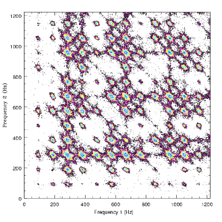
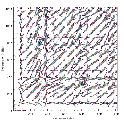
Figure 1: The bicoherences for case 1 (left) and case 2 (right), with no Poisson statistics corrections made. The contour levels for the squared bicoherence, $b^{2}$ are $10^{-1.0},10^{-1.5},10^{-1.75},10^{-2.0},10^{-2.25},$ and $10^{-2.65},$ in the colors red, green, dark blue, light blue, yellow, and purple, respectively. The frequencies correspond to a $10M_{\odot}$ black hole with spin parameter $a/M=0.5$. Note that the symmetry through the line $x$=$y$ is trivial.

Figure 2: The tracks showing how different harmonics of the QPO vary with respect to one another when the radius of the hot spot orbit varies around a central value $r\approx r_{0}\pm 0.2M$. The frequencies correspond to a $10M_{\odot}$ black hole with spin parameter $a/M=0.5$. Note that the symmetry through the line $x$=$y$ is trivial.

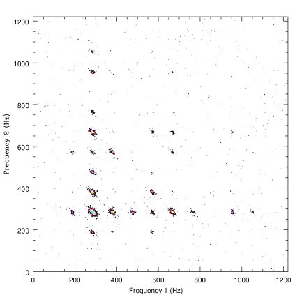
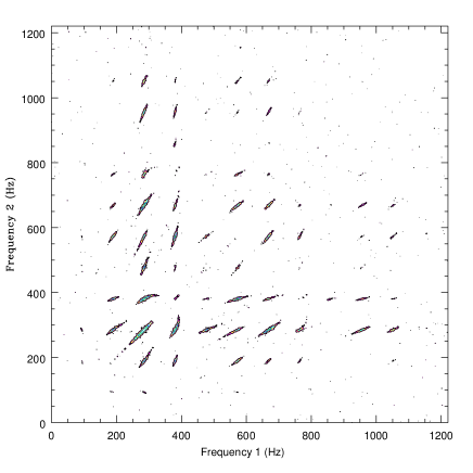
Figure 3: The bicoherences for case 1 (left) and case 2 (right), assuming 30 m² area for the detector and a 1000 second integration. The contour levels for the squared bicoherence, $b^{2}$ are $10^{-1.0},10^{-1.5},10^{-1.75},10^{-2.00},10^{-2.25},$ and $10^{-2.65},$ in the colors red, green, dark blue, light blue, yellow, purple, and black, respectively. The frequencies correspond to a $10M_{\odot}$ black hole with spin parameter $a/M=0.5$. Note that the symmetry through the line $x$=$y$ is trivial.

5 Simulations with Poisson Noise

To consider whether this observational test is really feasible, we have performed simulations with the rms amplitude of the oscillations reduced to realistic levels and with Poisson noise added. We consider two count rate regimes - one similar to that detected by RXTE for the typical X-ray transients at about 10 kpc, which is about 10,000 counts per second, and another which would be expected from the same source, but with a 30 m² detector. In each case, we allow 6% of the counts to come from the variable component and to have, intrinsically, count rates given by the simulated light curves of Schnittman (2004), and the remaining 94% of the counts to come from a constant component. We then simulate observed numbers of counts in 100 microsecond segments as Poisson deviates (Press et al. 1992) of the model count rates.

We then compute the bicoherence as above, but with 2440 segments of 4096 data points, for a total of 999.424 seconds of simulated data. For the RXTE count rates, we find that the bicoherence plots show only noise and only the strongest peak in the power spectrum is clearly significant in a 1000 second simulated observation, while marginal detections exist for the QPOs at two-thirds of and twice this frequency ($\nu_{\phi}-\nu_{r}$ and $2\nu_{\phi}$). This is as expected based on real data, which generally requires exposure times much longer than 1000 seconds to detect these QPOs. Longer simulated light curves have not been computed at this time due to computational constraints. However, since the signal-to-noise in the bicoherence should be substantially worse than the signal-to-noise in the power spectrum, bicoherence measurements should be possible only when a peak in the power spectrum is considerably stronger than the Poisson level.

For the count rates expected from a 30 m² detector, we find that even within 1000 seconds, several of the higher (i.e. $n>4$) harmonics are observable in the power spectrum and show the clear elongation in the bicoherence plot for case 2, indicating that proposed missions should be capable of making use of the bicoherence for studying HFQPOs. A few very weak peaks are seen in the bicoherence in case 1 even in 1000 seconds. The simulated bicoherences for a 30 $m^{2}$ detector are plotted in Figure 3. We note that these simulations are a bit over-simplified, in that we have not included the lower frequency QPOs and low frequency band-limited noise that are typically observed in conjunction with the HFQPOs, but that these variability components should not significantly affect the phase coupling of the high frequency QPOs. We also note that it might be possible to make use of the bicoherence even with RXTE if a more nearby X-ray transient goes into outburst, but that in such a case, the deadtime effects we have neglected here might become important.

6 Conclusions

We have shown here that the bicoherence can be useful in breaking the degeneracies between different QPO models which produce the same Fourier power spectrum. In particular, we have shown that in the context of a resonance model for the high frequency quasi-periodic oscillations seen from accreting black holes, the bispectrum is capable of distinguishing between broadening due to phase jitter caused by the rapid creation and destruction of hot spots and broadening due to an intrinsic distribution of physical frequencies in a broad range around a central value. In future work, we will examine the properties of the bicoherence for other models for these QPOs, such as oscillations in a pressure supported torus (Rezzolla et al. 2003). We note though that this diagnostic is likely to be useful only with new instrumentation (or the fortuitous outburst of a bright X-ray transient within about 3 kpc of the Sun). At the typical 10 kpc distances of X-ray transients, $RXTE$ is capable of detecting these QPOs generally only with rather long intergrations and careful selection of the photon energy bands to maximize the signal-to-noise, but proposed timing missions with considerably larger collections areas, like XTRA (e.g. Strüder et al. 2004) and the Relativistic Astrophysics Explorer (e.g. Kaaret 2002) should have considerably greater potential for making use of these statistics.

7 Acknowledgments

TM wishes to thank Marek Abramowicz, Wlodek Kluzniak, Shin Yoshida and Olindo Zanotti for stimulating discussions re-motivating his interest in X-ray variability; Phil Uttley and Simon Vaughan for discussions of statistical properties of the bispectrum; Mariano Mendez and Marc Klein Wolt for discussions of observational properties of HFQPOs; Ron Elsner for providing some useful background information on the bispectrum; and Luciano Rezzolla and Michiel van der Klis for comments on the manuscript as well as additional useful discussions. JDS would like to thank Edmund Bertschinger and Ron Remillard for many useful discussions, and would like to acknowledge support from NASA grant NAG5-13306.

References

- [1] Abramowicz, M.A., Czerny, B., Lasota, J.P. & Szuszkiewicz, E., 1988, ApJ, 332, 646
- [2] Abramowicz, M.A. & Kluzniak, W., 2001, A&A, 374L, 19
- [3] Bursa, M., Abramowicz, M.A., Karas, V. & Kluzniak, W., 2004, astro-ph/0406586
- [4] Chen, X. & Taam, R.E., 1995, ApJ, 441, 354
- [5] De Villiers, J.P., Krolik, J.H. & Hawley, J.F., 2003, ApJ, 599, 1238
- [6] Fackrell, J 1996, Ph.D. Thesis, University of Edinburgh
- [7] Greb, U. & Rusbridge, M.G., 1988, Plasma Physics and Controlled Fusion, 30, 537
- [8] Homan, J., Miller, J. M., Wijnands, R., van der Klis, M., Belloni, T.,Steeghs, D.,Lewin, W. H. G., 2004, ApJ, submitted (astro-ph/0406334)
- [9] Kaaret, P., 2002, COSPAR, 1240
- [10] Kato, Y., 2004, PASJ, in press
- [11] Li, L.-X. & Narayan, R., 2004, ApJL, 601, 414
- [12] Maccarone, T.J. & Coppi, P.S., 2002, MNRAS, 336, 817
- [13] Mendel, J. 1991, Proc IEEE, 79, 278
- [14] Miller, J.M., Wijnands, R., Homan, J., Belloni, T., Pooley, D., Corbel, S., Kouveliotou, C., van der Klis, M. & Lewin, W.H.G., 2001, ApJ, 563, 928
- [15] Nowak, M.A. & Vaughan, B.A., 1996, MNRAS, 280, 227
- [16] Nowak, M.A., Wagoner, R.V., Begelman, M.C. & Lehr, D.E., 1997, ApJL, 477, 91
- [17] Okazaki, A.T., Kato, S. & Fukue, J., 1987, PASJ, 39, 457
- [18] Press, W.H., Flannery, B.P., Teukolsky, S.A. & Vetterling, W.T., 1992, Numerical Recipes in FORTRAN, Cambridge University Press
- [19] Remillard, R.A., Morgan, E.H., McClintock, J.E., Bailyn, C.D. & Orosz, J.A., 1999, ApJ, 522, 397
- [20] Remillard, R.A., et al., 2002, ApJ, 580, 1030
- [21] Remillard, R.A., Muno, M.P., McClintock, J.E. & Orosz, J.A., 2003, HEAD, 35, 3003
- [22] Remillard, R.A., McClintock, J.E., Orosz, J.A. & Levine, A.M., 2004, ApJ, submitted (astro-ph/0407025)
- [23] Reynolds, C.S. & Nowak, M.A., 2003, PhR, 377, 389
- [24] Rezzolla, L., Yoshida, S’i., Maccarone, T.J., Zannotti, O., 2003, MNRAS, 344L, 37
- [25] Schnittman, J.D. & Bertschinger, E., 2004, ApJ, 606, 1098
- [26] Schnittman, J.D., 2004, ApJ, submitted (astro-ph/0407179)
- [27] Stella, L. & Vietri, M., 1999, PhRvL, 82, 17
- [28] Strohmayer, T.E., 2001, ApJL, 552, 49
- [29] Strüder, L., Barret, D., Fiorini,C., Kendziorra, E. & Lechner, P., 2004, SPIE, 5165, 19
- [30] Titarchuk, L., 2002, ApJL, 578, 71
- [31] Titarchuk, L., 2003, ApJ, 591, 354
- [32] Zanotti, O., Rezzolla, L. & Font, J.A., 2003, MNRAS, 341, 832