Stochastic Acceleration in Relativistic Parallel Shocks

Abstract

We present results of test-particle simulations on both the first and the second order Fermi acceleration (i.e., stochastic acceleration) at relativistic parallel shock waves. We consider two scenarios for particle injection: (i) particles injected at the shock front, then accelerated at the shock by the first order mechanism and subsequently by the stochastic process in the downstream region; and (ii) particles injected uniformly throughout the downstream region to the stochastic process mimicing injection from the thermal pool by cascading turbulence. We show that regardless of the injection scenario, depending on the magnetic field strength, plasma composition, and the employed turbulence model, the stochastic mechanism can have considerable effects on the particle spectrum on temporal and spatial scales too short to be resolved in extragalactic jets. Stochastic acceleration is shown to be able to produce spectra that are significantly flatter than the limiting case of $N(E)\propto E^{-1}$ of the first order mechanism. Our study also reveals a possibility of re-acceleration of the stochastically accelerated spectrum at the shock, as particles at high energies become more and more mobile as their mean free path increases with energy. Our findings suggest that the role of the second order mechanism in the turbulent downstream of a relativistic shock with respect to the first order mechanism at the shock front has been underestimated in the past, and that the second order mechanism may have significant effects on the form of the particle spectra and its evolution.

1 INTRODUCTION

For particle acceleration in astrophysical sources, such as jets and shock waves, two kinds of Fermi acceleration mechanisms have typically been considered: the first order Fermi acceleration at the shock fronts, and the second order Fermi acceleration (often referred to as stochastic acceleration) in the turbulent plasma. The first order mechanism is well known to produce a power-law particle spectrum $N(E)\propto E^{-s}$ with spectral index being a function $s=(r+2)/(r-1)$ of the compression ratio $r$ for non-relativistic shocks (e.g., Drury, 1983) and in relativistic shocks approaching the value $s\approx 2.2$ at the ultra-relativistic limit (e.g., Kirk et al., 2000; Achterberg et al., 2001; Lemoine & Pelletier, 2003; Virtanen & Vainio, 2003a), and it has been successfully applied in explaining the synchrotron properties of, e.g., some active galactic nuclei (AGN) (e.g., Türler et al., 2000). For flatter spectra ($s\lesssim 2$) the first order mechanism is not, however, as attractive. Although it can produce hard spectra with spectral index $s\to 1$ depending, for instance, on the injection model or the scattering center compression ratio (e.g., Ellison et al. 1990; Vainio, Virtanen & Schlickeiser 2003, hereafter referred to as VVS, 2003), it is not able to produce spectral indices flatter than $s=1$. Stochastic acceleration, on the other hand, has been known to exist and be present in the turbulent downstream of shocks, but because it works on much longer time scales than the first order mechanism (e.g., Campeanu & Schlickeiser, 1992; Vainio & Schlickeiser, 1998) it has been frequently neglected in studies of relativistic particle acceleration (however, note e.g., Ostrowski & Schlickeiser, 1993).

The argument of longer acceleration time scale renders the second order mechanism less important than the first order one, when the two mechanisms operate concurrently and, thus, the particle spectrum at the shock front is considered. When discussing non-thermal particle distributions radiating in astrophysical objects, however, it is important to acknowledge that the bulk of radiation is emitted by the particles that have already left the shock front towards the downstream. Thus, the second order mechanism has a much longer time available to accelerate the particles than the first order mechanism. Although one could justify the neglect of stochastic acceleration when calculating the particle spectrum right at the shock front, it is not possible to neglect its effect on the spectrum of radiating particles in astrophysical shock waves in general as these objects, especially those believed to host relativistic shock waves, are often spatially unresolved.

In this paper we have studied the possible effects of stochastic electron acceleration in parallel relativistic shock waves. We approach the subject via numerical test-particle simulations and present our model including both the first and the second order Fermi acceleration. We employ the model to study the effect of stochastic acceleration on (i) particles injected at the shock front and subsequently accelerated by the first order mechanism and (ii) particles drawn from the heated (but not shock accelerated) particle population of the downstream region of the shock. We focus on shock waves that, in addition to being parallel, have small-to-intermediate Alfvénic Mach numbers. Low Mach-number relativistic shocks could prevail in magnetically dominated jets that are lighter than their surroundings, e.g., because of having a pair-plasma composition.

The structure of this paper is as follows. In §2 we present our model, state the limiting assumptions we have made, and briefly discuss the limitations caused by the assumptions and simplifications; the description of the numerical code, as well as the implementations and mathematical details of the underlying physics are described in Appendix A. In §3 we present the results achieved using the simulation code. We begin by showing that when compared to some relevant previous studies – both analytical and numerical – our results are in very good accordance with those achieved previously by many authors. We then continue presenting the results for stochastic acceleration in various cases, and in §4 we discuss our results and their relationship to both the previous studies and possible future applications, and list the conclusions of our study. Also the limitations caused by the test-particle approach are shortly discussed.

2 MODEL

In this section we describe the properties of our model in general, including the employed assumptions and physics related to them. The numerical Monte-Carlo approach is described in detail in Appendix A, where also implementations of the model properties are discussed.

2.1 Coordinate systems

Before proceeding into the model, we define the coordinate systems employed in our study: the frame where the shock front is at rest is called the shock frame. We consider parallel shocks, i.e., shocks where the mean magnetic field and the plasma flow are directed along the shock normal. The frame where the bulk plasma flow is at rest is called the local plasma frame; this frame moves with the local flow speed, $V$, with respect to the shock frame. Finally, we consider the wave frame, which moves with the phase speed $V_{\phi}$ of the plasma waves with respect to the local plasma frame and, thus, at speed $(V+V_{\phi})/(1+VV_{\phi}/c^{2})$ with respect to the shock frame denoting, as usual, the speed of light by $c$. If the scattering centers are taken to be fluctuations frozen-in to the plasma then the speed of the waves with respect to the underlying plasma flow is $V_{\phi}=0$ and the plasma frame is also the rest frame of the scattering centers.

2.2 Shock Structure

We use the hyperbolic tangent profile of Schneider & Kirk (1989) to model the flow velocities at different distances from the shock. The width of the transition from the far upstream flow speed, $V_{1}$, to that of the far downstream, $V_{2}$, takes place over a distance of $0.01\lambda_{\rm e}(\Gamma_{1})$ (for which the shock can still be considered almost step-like; see, e.g., Virtanen & Vainio 2003a), where $\lambda_{\rm e}(\gamma)$ denotes the mean free path of the electrons as a function of Lorentz factor

$$\gamma=1/\sqrt{1-(v/c)^{2}},$$ (1)

$v$ is the electron speed, and $\Gamma_{1}$ is the Lorentz factor of the upstream bulk flow. (We use the standard notation of subscript 1[2] denoting the upstream [downstream] values.) The ratio of the flow speeds on both sides of the shock gives the gas compression ratio

$$r=\frac{V_{1}}{V_{2}}.$$ (2)

We fix the shock speed in the upstream rest frame and, thus, the (equal) upstream bulk speed $V_{1}$ in the shock frame. Using this we compute the corresponding gas compression ratio for a given shock proper speed

$$u_{1}=c\sqrt{\Gamma_{1}^{2}-1}$$ (3)

following a scheme described by VVS (2003) and shown in Figure 1. Finally, the flow speed in the far downstream $V_{2}$ is given by equation (2).

Figure 1: Gas compression ratio $r$ in a parallel shock propagating into a cold medium with proper speed $u_{1}$ (VVS, 2003).

2.3 Magnetic Field and Scattering

For modeling the magnetic field structure we adopt the quasilinear approach, where the field $B$ is considered to consist of two parts: the static, large scale background field $B_{0}$, and smaller scale fluctuations with amplitude $\delta B<B_{0}$. We model the turbulence as being composed of a wide-band spectrum of Alfvén waves propagating both parallel and anti-parallel to the flow. In the local plasma frame the waves propagate at Alfvén speed

$$v_{\rm A}=\frac{B_{0}c}{\sqrt{4\pi hn+B_{0}^{2}}}$$ (4)

where $h=(\rho+P)/n\equiv w/n$, $n$, $\rho$, and $P$ are the specific enthalpy, the number density, the total energy density, and the gas pressure – all measured in the local plasma frame. The wave intensity as a function of wavenumber, $I(k)$, is assumed to have a power-law form for wavenumbers above an inverse correlation length $k_{0}.$ We write the power-law as

$$I(k)=I_{0}(k_{0}/k)^{q},\;k>k_{0}$$ (5)

where $q$ is the spectral index of the waves. For wavenumbers smaller than $k_{0}$ the wave intensity per logarithmic bandwidth is assumed to be equal to the background field intensity, i.e., $I(k)=B_{0}^{2}k^{-1}$ for $k<k_{0}$. In this work we use two values for $q$: $2$ and $5/3$. The former produces rigidity independent scattering mean free paths, while the latter is consistent with the Kolmogorov phenomenology of turbulence.

Electrons scatter off the magnetic fluctuations resonantly. The scattering frequency of electrons with Lorentz factor $\gamma$ is determined by the intensity of waves at the resonant wavenumber (see Appendix A.)

$$k_{{\rm res}}=\frac{\Omega_{{\rm e}}}{v}=\frac{\Omega_{{\rm e},0}}{c\sqrt{\gamma^{2}-1}},$$ (6)

where

$$\Omega_{{\rm e}}=\frac{\Omega_{{\rm e,0}}}{\gamma}$$ (7)

is the relativistic electron gyrofrequency, and $\Omega_{\rm e,0}=\frac{eB}{m_{{\rm e}}c}$ is its non-relativistic counterpart.

Scatterings are elastic in the wave frame and the existence of waves propagating in both directions at a given position, thus, leads to stochastic acceleration (Schlickeiser, 1989). Since the spectrum of waves is harder below $k=k_{0}$, scattering at energies

$$\gamma>\gamma_{0}\equiv\frac{\Omega_{{\rm e,0}}}{k_{0}c}\gg 1$$ (8)

becomes less efficient. Thus, we expect the electron acceleration efficiency to decrease at $\gamma>\gamma_{0}$. Instead of trying to fix the value of $k_{0}$, we use a constant value $\gamma_{0}=10^{6}$, which corresponds to observations of maximum Lorentz factor of electrons in some AGN jets (Meisenheimer et al., 1996).

In addition to scattering, the particles are also assumed to lose energy via the synchrotron emission. The average rate of energy loss for an electron with Lorentz factor $\gamma$ in the frame co-moving with the plasma is given by

$$\frac{dE}{dt}=-\frac{4}{3}\sigma_{{\rm T}}c\gamma^{2}U_{B},$$ (9)

where $\sigma_{{\rm T}}$ is the Thompson cross-section and $U_{B}=B_{0}^{2}/(8\pi)$ is the magnetic field energy density. We calculate the latter in all simulations by assuming a hydrogen composition of the plasma.

2.4 Alfvén-Wave Transmission

Downstream Alfvén-wave intensities can be calculated from know upstream paramters (e.g., Vainio & Schlickeiser, 1998; VVS, 2003). Regardless of the cross helicity of the upstream wave field (only parallel or anti-parallel waves, or both), there are always both wave modes present in the downstream region. The transmission coefficients for the magnetic field intensities of equation (5) of forward $(+)$ and backward $(-)$ waves at constant wavenumber $\tilde{k}$, measured in the wave frame, can be written (see VVS, 2003, equations (22) and (23)), as

$$\tilde{T}_{\tilde{k}\pm}^{2}\equiv\frac{\tilde{I}_{2}^{\pm}(\tilde{k})}{\tilde{I}_{1}^{\pm}(\tilde{k})}\hskip 14.22636pt{\rm and}\hskip 14.22636pt\tilde{R}_{\tilde{k}\pm}^{2}\equiv\frac{\tilde{I}_{2}^{\mp}(\tilde{k})}{\tilde{I}_{1}^{\pm}(\tilde{k})}.$$ (10)

Using these we can solve the amplification factor of the wave intensity for both wave modes for constant wave frame wave number $\tilde{k}$ as

$$\tilde{W}_{\tilde{k}\pm}=\tilde{T}_{\tilde{k}\pm}^{2}+\tilde{R}_{\tilde{k}\mp}^{2}.$$ (11)

Amplification factor depends on the strength of the magnetic field as well as on the form of the turbulence spectrum. The intensity ratio of the backward waves to that of forward waves as a function of the quasi-Newtonian Alfvénic Mach number,

$$M=u_{1}/u_{{\rm A,1}},$$ (12)

is plotted in Figure 2 for three different Alfvén proper speed

$$u_{{\rm A,1}}=v_{{\rm A,1}}/\sqrt{1-\beta_{{\rm A,1}}^{2}},$$ (13)

where $\beta_{{\rm A,1}}=v_{{\rm A,1}}/c$. The waves are seen to propagate predominantly backward for relatively low-Mach-number shocks as shown by VVS (2003) in case of relativistic shocks, and by Vainio & Schlickeiser (1998) for non-relativistic shocks. This enables the scattering center compression ratio $r_{k}$ to grow larger than the gas compression ratio $r$ and, thus, to cause significantly harder particle spectra compared to the predictions of theories relying on fluctuations frozen-in to plasma flow. As the Mach number increases, the downstream wave intensities approach equipartition at the ultra-relativistic limit.

Figure 2: Ratio of the amplified wave intensities as function of Alfvénic Mach number. Cases corresponding to proper Alfvén speeds $u_{{\rm A,1}}$ of $10.0\,c$, $1.0\,c$, and $0.1\,c$ are plotted with solid, dotted, and dashed lines, respectively, in the case of Kolmogorov turbulence, to $q=5/3$.

Waves conserve their shock-frame frequencies during the shock crossing (Vainio & Schlickeiser, 1998), and for given upstream wave-frame wavenumbers $\tilde{k}_{1\pm}$ (here equipartition of the upstream waves is assumed) the downstream wave frame values are obtained from (VVS, 2003)

$$\tilde{k}_{2+}=\frac{\Gamma_{1\pm}V_{1\pm}}{\Gamma_{2+}V_{2+}}\tilde{k}_{1\pm};\quad\tilde{k}_{2-}=\frac{\Gamma_{1\pm}V_{1\pm}}{\Gamma_{2-}V_{2-}}\tilde{k}_{1\pm}$$ (14)

for both the forward ($\tilde{k}_{2+}$) and the ($\tilde{k}_{2-}$) waves. Here $V_{j\pm}$ and $\Gamma_{j\pm}$ refer to the wave speeds of forward (+) and backward ($-$) waves in the upstream ($j=1$) and downstream ($j=2$) region and to the respective Lorentz factors. The functional form of the spectrum does not change on shock crossing and the spectral index $q$ in equation 5 is the same both sides of the shock.

2.5 Testing the Model

We have tested the ability of our model to produce results expected from previous numerical studies and theory. To test the model in the case of first order acceleration we ran numerous test-particle simulations with different injection energies and shock widths (Virtanen & Vainio, 2003a, b). We found our results to be in very good agreement with the semi-analytical results for modified shocks of Schneider & Kirk (1989), as well as to the numerical results of, e.g., Ellison et al. (1990) for the corresponding parts of the studies. For the step-shock approximation, spectra with indices close to the predicted value of $\sim 2.2$ were obtained. An example of the test-runs is shown in Figure 3 with the shock proper speed $u_{1}=10\,c$ and compression ratio $r\approx 3$, assuming scattering centers frozen-in into the plasma and turbulence having a spectral index of $q=2$.

Figure 3: Spectrum of the particles accelerated at the shock front in the step-shock approximation. Resulting spectral index for power-law – extending over five orders of magnitude in energy – is $s\simeq 2.2$.

For testing the second order acceleration we chose an analytically well known case, namely that of uniform flow with waves streaming in parallel and anti-parallel directions with equal intensities. In this case the momentum diffusion coefficient of charged particles can be given as (Schlickeiser, 1989)

$$A_{2}(x,p)\simeq\frac{2\pi\Omega_{{\rm e}}^{2-q}k_{0}^{q}I_{0}}{q(q+2)B_{0}^{2}}\frac{p^{2}v_{{\rm A}}^{2}}{v^{3-q}},$$ (15)

which in the relativistic case ($v\approx c$ and $p\gg m_{{\rm e}}c$) is found to depend on the momentum $p$ as

$$A_{2}\propto p^{q}.$$ (16)

For a constant particle injection at low momenta, this leads to a simple relation of the spectral index of the volume-integrated particle energy spectrum, $s$, and the magnetic field fluctuations, $q$:

$$s=q-1.$$ (17)

As a test case, we ran simulations involving only stochastic acceleration, and found that for values $q\in[1,2]$ the model produces exactly those indices expected from the analytical calculation. The spectral indices obtained from the simulation are plotted together with the theoretical prediction in Figure 4.

Figure 4: Comparison of the simulation model and the theory. Spectral index of the energy spectrum of particles accelerated stochastically for different spectral indices of the magnetic field fluctuations. Data from the simulations are plotted with crosses (statistical error of each plot is $0.02$ or less), and the theoretical prediction of $s=q-1$ is plotted as a straight line.

3 RESULTS

In this section we apply our model to stochastic particle acceleration in the downstream region of a relativistic parallel shock, using a test-particle approach.

First we show how the stochastic process affects a non-thermal particle population, already accelerated at the shock via the first order mechanism. Then we consider particles injected throughout the downstream region. Finally we present an example of the combination of both injection schemes. Simulations were run separately for low, intermediate and high Alfvénic-Mach-number shocks ($M=3$, $M=10,$ and $M=1000$, respectively – see Fig. 2 for the corresponding wave intensity ratios), and for four cases of downstream turbulence; for turbulence spectral index $q=2$ and $q=5/3$ with downstream wave field calculated using wave transmission analysis described in §2.4, and with the downstream forward and backward waves being in equipartition. The proper speed of the shock is set to $u_{1}=10\,c$ in all simulations.

3.1 Electrons Injected and Accelerated at the Shock

We have studied the effect of stochastic acceleration on particles that have been already accelerated at the shock. This was done by injecting particles into the shock and the first order mechanism, and allowing them to continue accelerating via the stochastic process in the downstream region. Injection of the particles took place in the downstream immediately after the shock, and particles were given an initial energy of a few times the energy of the thermal upstream particles as seen from the downstream. This kind of injection simulates some already-energized downstream particles returning into the shock, but without the need of processing the time consuming bulk of non-accelerating thermal particles. The high-energy part of the particle energy distribution – which we are interested in in this study – is similar, regardless of the injection energy.

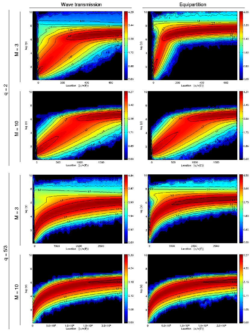
Figure 5: Evolution of the particle spectra in the turbulent downstream region due to stochastic acceleration. Particles are initially injected and accelerated at the shock front, located at $x=0$ near the left edge of the plots. Contours of $\log(E\frac{dN}{dE})$ show the steady-state particle energy distribution. On the left-hand panels the wave transmission calculation of VVS (2003) is applied, whereas on the right-hand panels the downstream waves modes are assumed to be in equipartition. In the two uppermost rows $q=2$, and in the two lowermost panels $q=5/3$. Results for Alfvénic Mach numbers $M=3$ (first and third row) and $10$ (second and fourth row) are shown for each case. The physical sizes of the downstream region are approximately $10^{12}$ cm (first row), and $10^{13}$ cm (second row) for the $q=2$ cases, and $10^{11}$ cm (third row), and $10^{12}$ cm (fourth row) for the $q=5/3$ cases.

We found that in the case of high Alfvénic Mach number ($M=1000$, corresponding to magnetic field $B_{0}\simeq 1.4$ mG in a hydrogen plasma) the contribution of the stochastic process to the energy distribution of the particles is, indeed, very insignificant compared to that of the first order acceleration at the shock; the energy spectrum maintains its shape and energy range unaltered at least for tens of thousands thermal electron mean free paths. This is the case regardless of the applied turbulence spectral index, and because the analytically calculated wave intensities are very close to equipartition for high-Mach-number shock (see Fig. 2), the difference between the analytically calculated downstream wave field and the explicitely assumed equipartition case was, as expected, minimal.

For stronger magnetic fields ($M=10$ and $M=3$, corresponding to $0.14$ G and $0.46$ G, respectively, in a hydrogen plasma, and to $4.6$ mG and $15$ mG in a pair plasma) the effect of stochastic acceleration is, on the contrary to the high-$M$ case, very pronounced. The stochastic process begins to re-accelerate particles immediately after the shock front, and the whole spectrum slowly shifts to higher energies as shown in Figure 5, where the results obtained using wave transmission analysis are presented in the left-hand column, while the right-hand panels show the results of the equipartition assumption. The acceleration rate depends on the wave spectrum in a way that for $q=2$, for which particles of all energies have the same mean free path, the stochastic process accelerates particles to higher energies at constant rate, whereas for the Kolmogorov turbulence the acceleration rate (like the mean free path of the particles) decreases as the energy increases, and the energization gradually slows down as the bulk of the particle energy distribution rises to higher energies. Also different composition of the downstream wave field leads to slightly different results: in the “transmitted” case (left-hand panels) the particle population immediately behind the shock front extends to slightly higher energies than in the equipartition case (right-hand panels), but for the latter the stochastic acceleration is clearly quicker. This can be seen best in the uppermost panels of Figure 5, where the calculated transmitted wave field differed from the equipartition assumption the most.

Figure 6: Energy distribution of the particles escaping the shock region and getting absorbed in the downstream. The Alfvénic Mach number of the shock is $M=10$, the proper speed is $u_{1}=10\,c$, and the turbulence corresponds to $q=5/3$. Note that the distribution is plotted as $\log(dN/dE)$.

The “turnover” of the scattering rate at energy $\gamma_{0}=10^{6}$ causes the rate of energization to go down for energies greater than $\gamma_{0}$. This is because the energy dependence of the mean free path of the particle changes when particles resonant wavenumber (eqn. (6)) decreases below $k_{0}$, which was use to set the lower limit for the $I(k)\propto k^{-q}$ power-law. For particles with $\gamma>\gamma_{0}$ the mean free path starts to increase much faster, leading not only to the decrease of the stochastic acceleration efficiency, but also to another notable effect: as its scattering mean free path increases at $\gamma>\gamma_{0}$, the particle will suddenly be able to move much more easily in the downstream region and even be able to return back to the shock. Particles already energized first in the shock by the first order mechanism and then in the downstream by the second order acceleration, and returning back into the shock again, get “re-injected” into the first order acceleration process. This effect, in general, is seen in all simulations with $M=3$ as a bending of the countours to the left at $\gamma>\gamma_{0}$ close to the shock (at $x=0$), but it is visible also in $M=10$ shocks in spectra of particles collected at the downstream free-escape boundary. An example of the latter case is shown in Figure 6.

3.2 Electrons Injected from the Downstream Bulk Plasma

Our second approach was to assume that a constant injection mechanism exists throughout the downstream region and investigate the stochastic acceleration process. (Physically, this mimics a case, where turbulent fluctuations cascade to higher wavenumbers and inject a fraction of the thermal electrons to the stochastic acceleration process.) We injected particles at constant energy – corresponding to the energy equal to the energy of upstream electrons as seen from the downstream region – uniformly and isotropically within the whole downstream region. The results for different cases are shown in Figure 7.

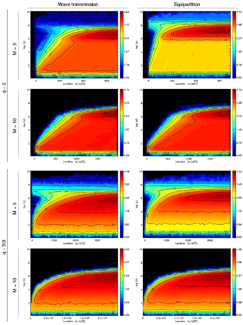
Figure 7: Same as Fig. 5 but for particles injected uniformly and isotropically across the downstream region.

The Figure shows similar behavior as in the case of particles injected at the shock: significant acceleration was seen only for shocks with strong magnetic field, while in the $M=1000$ case practically no acceleration is seen. For the cases with strong magnetic field the acceleration is seen to work similarly as in the previous shock-related injection case, energizing particles at constant rate for $q=2$ turbulence, and with decreasing rate for $q=5/3$. Again the acceleration rate slows down when energies corresponding to $\gamma_{0}$ are reached. After this energy particles start to pile up and form a bump in the distribution immediately behind the $\gamma_{0}$. Also here (at least for $M=3$) some particles with energy $\gamma>\gamma_{0}$ are able to return to the shock and get re-injected to the first order process (see, e.g., the right-hand panel of Fig 8).

In the energy range between the injection energy and $\gamma_{0}$, particles begin to form a power-law distribution with spectral index depending on the magnetic field fluctuations, as expected from equation (17). For $q=2$, the particle spectral index $s\simeq 1$, and for $q=5/3$, $s\simeq 0.6$. The formation of the power laws as function of distance from the shock is shown in the left-hand panel of Figure 8 for $q=2$, and in the right-hand panel for $q=5/3$. In the latter case also the formation of high-energy bump at the shock by the returning accelerated particles is seen.

Figure 8: Energy spectrum of the particles at different distances from the shock. The particles are injected in the downstream region and the distributions are from the simulation with $q=2$ and $M=10$ (wave field transmitted) for the left-hand panel and from $q=5/3$ and $M=3$ (wave field in equipartition) for the right-hand panel (corresponding to the left-hand panel of the second row and the top right panel of Fig. 7). Slices are from locations $x=0$ (solid line), $x=100$ (dashed), $x=400$ (dotted), $x=1000$ (dash-dotted), and $x=2000$ (dash-dot-dot-dotted) for the left-hand panel, and from $x=0$ (solid line), $x=300$ (dashed), $x=600$ (dotted), $x=1500$ (dash-dotted), and $x=3000$ (dash-dot-dot-dotted) for the right-hand panel.

3.3 Example of Combination

We have investigated what kind of particle energy spectra the two discussed injection schemes – one operating at the shock, and another operating uniformly throughout the downstream region – are able to create. Next we will present an example of a combination of these. In the simulation these two cases were kept separate for the sake of simplicity, but there should be no reason to assume the separation be present also in nature. Also the relative amounts of shock-injected and downstream-injected particles is not fixed here, but instead considered more or less free a parameter.

Assuming different ratios of injected particle populations, the resulting spectrum would be very different. An example of combination of the two injection schemes in the case of shock with $u_{1}=10\,c$ and $M=10$, and with turbulence corresponding to $q=5/3$, is shown in Figure 9.

Figure 9: Example of a combination (solid line) energy spectra of particles injected to the acceleration process at the shock (dashed) and throughout the downstream region (dotted). (Model parameters are $q=5/3$ and $M=10$.) The particles are collected at the downstream free escape boundary, $\sim 4\times 10^{12}$ cm away from the shock, and the number of the particles injected at the shock is larger than the number of uniformly injected particles by a factor of $100$.

4 DISCUSSION AND CONCLUSIONS

We have studied stochastic particle acceleration in the downstream region of a relativistic parallel shock. Applying the wave transmission calculations of VVS (2003) and assuming the cross helicity to vanish in the upstream, we have modeled the turbulence of the downstream region as a superposition of Alfvén waves propagating parallel and anti-parallel to the plasma flow. Using a kinetic Monte-Carlo simulation we have modeled the second order Fermi acceleration of electrons in the shock environment, and considered cases of acceleration of downstream-injected particles, as well as that of particles injected at the shock. We have shown that the stochastic acceleration can, indeed, have remarkable effects in both cases. This result is even more pronounced if the two downstream Alfvén wave fields are assumed to be in equipartition.

The behavior of the particle energy distribution in the stochastic process depends heavily on the strength of the background magnetic field; in the cases of weak magnetic field and quasi-Newtonian Alfvénic Mach number much larger than the critical Mach number ($M\gg M_{\rm c}=\sqrt{r}$) the effects of stochastic acceleration are faded out by the much stronger first order acceleration. Also the magnetic field turbulence spectrum affects the acceleration efficiency: for Kolmogorov turbulence with $q=5/3$ the spatial scales are up to an order of magnitude shorter than in the case of $q=2$ turbulence. Although the spatial scales in simulations presented here are enormous compared to those associated with shock acceleration (the first order process in the immediate vicinity of the shock front), in case of blazars and other AGNi the scales are still orders of magnitude too small to be resolved even in the VLBI pictures – regardless of the turbulence and used magnetic field strength. Also the acceleration time scales are very short: the time required to shift the whole spectrum from the initial energy range to $\gamma_{\rm bulk}\gtrsim 10^{6}$ ranged from $10$ to $50$ minutes in the $M=10$ case, and for $M=3$ the times were $\lesssim 1$ minute, as measured in the shock frame.

In addition to the magnetic field strength and turbulence, also the composition of the downstream wave field was seen to affect the resulting particle population. When comparing otherwise similar cases that differ only for the downstream cross helicity (i.e., whether the wave field is resulting from the wave transmission calculations of VVS (2003) or an equipartition of parallel and anti-parallel waves is assumed), the calculated wave-transmission cases with more anti-parallel waves (VVS, 2003, and Fig.2) showed stronger first order acceleration, but weaker stochastic acceleration. This is because of the larger scattering center compression ratio in the wave-transmission case leading to more efficient first order acceleration (VVS, 2003) and, on the other hand, faster momentum diffusion rate in the equipartition case leading to more efficient stochastic acceleration.

In the cases where the stochastic acceleration was quick enough for particles to reach the $\gamma_{0}$ energy while being still sufficiently close to the shock in order to be able to make their way back to the upstream region due to their prolonged mean free path, the first order mechanism was able to re-accelerate the returning high-energy particles to even higher energies. This led to forming of a new (quasi-)power-law at energies $\gamma\gtrsim 10^{7}$ in some cases.

One notable feature of the present model is that in the case of a uniform injection process in the downstream region, power-law spectra with high and low energy cut-offs are formed. Depending on the turbulence, particle energy spectra have power-law spectral indices of $0.5$–$1$ with lower and higher energy cut-offs at $\gamma_{1}\approx 10^{1}\simeq\gamma_{\rm injection}$ and $\gamma_{2}\sim 10^{6}=\gamma_{0}$, respectively. These particles would produce synchrotron spectra with photon spectral indices $-0.5<\alpha<0$ in the GHz–THz regime for various initial parameters. These properties are quite similar to those of flat-spectrum sources, for which typical spectra with $\alpha\gtrsim-0.5$ in the GHz region and flare spectra with $\alpha\approx-0.2$ in the optically thin region of the spectrum are seen (e.g., Valtaoja et al., 1988, and references therein).

Combining the resulting energy distributions of both the particles injected at the shock and the particles injected uniformly in the downstream region can lead to very different results depending on the relative amounts of particles injected in both cases. Because different distributions produce various observable spectra, one might, in principle, be able to set constraints on different injection mechanisms, as well as the physical size of the turbulent downstream region of the shock, comparing the evolution of observed radiated spectra and the predictions basing on several composite distributions. Especially the maximum Lorentz factor of electrons could be used to set limits for $\gamma_{0}$, as well as the lowest-energy parts of the non-thermal power-law spectra could give hints of the injection process.

Our simulations are based on test-particle approximation, i.e., the effects of the particles on the turbulent wave spectrum and on the shock structure are neglected. Including wave-particle interactions in a self-consistent manner may modify the cross-helicities and wave intensities in the downstream region and lead to notable effects on the accelerated particle spectrum (e.g., Vainio, 2001). One should note, however, that the wave particle interactions are competing with wave-wave interactions in the turbulent downstream region, which may modify the the turbulence parameters in a different manner. Including these effects to our model are, however, beyond of the scope of the present simulations.

To conclude, the main results of this paper are: (i) Stochastic acceleration can be a very efficient mechanism in the downstream region of parallel relativistic shocks, provided that the magnetic field strength is large enough in order to make the Alfvénic Mach number approach the critical Mach number ($M_{\rm c}=\sqrt{r}$) of the shock, i.e., to increase the downstream Alfvén speed enough to allow for sufficient difference in speeds of parallel and anti-parallel Alfvén waves required for rapid stochastic acceleration. (ii) The forming of a power-law with very hard particle energy spectra between the injection energy and $\gamma_{0}$ in the case of a continuous injection mechanism in the downstream region. The produced particle populations could produce synchrotron spectra very similar to those of flat spectrum sources. (iii) The interplay between the first and second order Fermi acceleration at relativistic shocks can produce a variety of spectral forms not limited to single power laws.

Appendix A. The Monte Carlo Code

In this appendix we review the structure and implementation of our simulation code. The code employs a kinetic test-particle approach; it follows individual particles in a pre-defined and simplified shock environment, based on the assumptions and simplifications presented in § 2. In short, the simulation works as follows: we trace test particles under the guiding center approximation in a homogeneous background magnetic field with superposed magnetic fluctuations. The fluctuations are assumed to be either static disturbances frozen-in into the plasma flow, or Alfvén waves propagating along the large-scale magnetic field parallel and antiparallel to the flow (in this paper we apply only the Alfvén wave case). In each time-step the particle is moved and scattered; scatterings are modeled as pitch-angle diffusion with an isotropic diffusion coefficient $D_{\mu\mu}\propto 1-\mu^{2}$, where $\mu=\cos\theta$ is the pitch-angle cosine of the particle. Also for each simulation time-step the energy losses due to the synchrotron emission (see eq. (9)) are calculated.

When the particle passes a free-escape boundary in the far downstream region it is removed from the simulation. The injection of the particles into the simulation is modeled using several methods. The first method involves a uniform and isotropic injection of particles within one mean free path of a thermal electron downstream of the shock front, simulating the already-energized supra-thermal particles crossing and re-crossing the shock. This injection method allows us to concentrate on the non-thermal particles without having to spend most of the computing time simulating the thermal body of the total particle distribution. Other injection employed methods include an injection of a cold distribution upstream, or an injection of particles at thermal energies uniformly and isotropically in the downstream region (the latter case is applied in §3.2).

The time unit of the simulation is chosen to be the inverse of the scattering frequency of an electron having energy $E_{\Gamma_{1}}\equiv\Gamma_{1}m_{\rm e}c^{2}$, where $\Gamma_{1}$ is the Lorentz factor of the shock. The unit of velocity is chosen as $c$. With these choices the unit of length equals the mean free path of electron with Lorentz factor that of the shock: $\lambda_{\rm e}(\Gamma_{1})=1/\nu_{\rm e}(\Gamma_{1})$. The time-step is chosen so that it is a small fraction of the inverse scattering time, $\Delta t=a\nu_{\rm e}(\gamma)$, where $a\lesssim 0.01$.

For a typical simulation $\sim 10^{5}$ particles are injected. The number of high-energy particles is further increased by applying a splitting technique; if the energy of a particle exceeds some pre-defined value, the particle is replaced by two ”daughter particles” which are otherwise identical to their ”mother”, but have their statistical weight halved. The number of these splitting boundaries is chosen so that for each simulation the balance between the statistics and the simulation time is optimal.

A.1. The Shock and the Flow Profile

We consider a shock wave propagating at speed $V_{1}$ into a cold ambient medium, which is taken to be initially at rest in the observer’s frame. In the shock frame the shock is, by definition, at rest and the upstream plasma flows in with speed $V_{1}$. At the shock front the plasma slows down, undergoes compression, and flows out at downstream flow speed $V_{2}<V_{1}$. The shocked downstream values of the plasma parameters are determined by the compression ratio of the shock defined in equation (2).

For the flow speed depending on the location $x$, we use the hyperbolic tangent form of Schneider & Kirk (1989),

$$V(x)=V_{1}-\frac{V_{1}-V_{2}}{2}\left[1+\tanh\left(\frac{x}{W\lambda_{\rm e}(\Gamma_{1})}\right)\right],$$ (18)

and fix the shock thickness to $W=0.01$, corresponding to a nearly step-like shock. For thicker shocks the first order acceleration efficiency drops fast (e.g. Schneider & Kirk, 1989; Virtanen & Vainio, 2003b), and also the simple wave-transmission calculations of VVS (2003) would not be valid.

A.2. Magnetic Field

The strength of the parallel magnetic field, $B_{0}$, in the simulation is defined with respect to the ”critical strength” for which the Alfvén speed in the downstream region becomes equal to the local flow speed; for fields stronger than this the parallel shock becomes non-evolutionary. The critical field, $B_{\rm c}$, is calculated from equation

$$B_{\rm c}c/\sqrt{4\pi h_{2}n_{2}+B_{c}^{2}}=V_{2},$$ (19)

for which we get the downstream particle density $n_{2}$ and the specific enthalpy $h_{2}$ using the magnetohydrodynamical jump conditions (e.g., Kirk & Duffy, 1999) and the upstream values $n_{1}=1\ {\rm cm^{-3}}$ and $h_{1}=(\rho_{1}+P_{1})/n_{1}=mc^{2}$ with $m=m_{\rm e}+m_{\rm p}$ in a hydrogen plasma and $m=2m_{\rm e}$ in a pair plasma (throughout this work the upstream plasma is assumed to be cold so that its pressure may be neglected compared to its rest energy). Applying the equations for conservation of both energy

$$h_{1}\Gamma_{1}V_{1}=h_{2}\Gamma_{2}V_{2}$$ (20)

and mass

$$\Gamma_{1}V_{1}n_{1}=\Gamma_{2}V_{2}n_{2},$$ (21)

and a bit of straightforward algebra, the critical field can be written as

$$B_{\rm c}=\sqrt{4\pi V_{1}V_{2}mn_{1}}\,\Gamma_{1}.$$ (22)

For example, for a shock with compression ratio $r=3$ propagating into a cold ambient medium of $n_{1}=1\,{\rm cm^{-3}}$ at proper speed $u_{1}=10\,c$ the critical field is $B_{\rm c}\approx 0.8\,{\rm G}$ for a hydrogen plasma and $0.03$ G for a pair plasma.

A.3. Particle Transport and Scattering

During each Monte Carlo time-step scatterings off the magnetic fluctuations are simulated by making small random displacements of the tip of the particle’s momentum vector, and the particle is transported according to its parallel (to the flow) speed in the fixed shock frame. In the case of stochastic acceleration, the particle is scattered twice for each Monte Carlo time-step. Instead of only one scattering off scattering centers frozen-in into the plasma, the scattering process is now divided into two parts: the particle is first scattered in the forward-wave frame, and then immediately again in the backward-wave frame. The scattering frequencies of both scatterings are adjusted so that the total statistical effect of the duplex scattering is consistent with the value of the momentary scattering mean free path. This is done by balancing the both scattering frequencies by weight values $\omega_{\pm}\in[0,1]$, which are calculated from the ratio of the amplified waves (eq. 11 and Fig. 2), so that they satisfy the relation $\omega_{+}+\omega_{-}=1$. Neglecting, for simplicity of the simulations, the dependence of the scattering frequency on the particle’s propagation direction, and assuming that the scattering is elastic in the rest frame of the scattering centers, we can use the quasilinear theory: the scattering frequency of an electron as a function of its Lorentz factor (in the rest frame of the scattering centers, denoted here by prime) $\gamma^{\prime}$ is

$$\nu(\gamma^{\prime})\approx\frac{\pi}{2}\frac{\Omega_{0}}{\gamma^{\prime}}\frac{k^{\prime}I^{\prime}(k^{\prime})}{B^{2}}\propto\frac{\left(\gamma^{\prime 2}-1\right)^{(q-1)/2}}{\gamma^{\prime}}.$$ (23)

This equation is applicable to particles scattering off waves with wavenumber larger than $k_{0}$; for particles with Lorentz factor $\gamma^{\prime}>\gamma^{\prime}_{0}$ the scattering frequency decreases as $\nu\propto\gamma^{-1}$, as at these wavenumbers $k^{\prime}I(k^{\prime})=B_{0}^{2}$ is assumed. Scattering frequency as a function of particle’s Lorentz factor is plotted in Figure 10 for magnetic field fluctuations with $q=2$ (leading to energy-independent mean free path) and $q=5/3$.

Figure 10: Scattering frequency as a function of Lorentz factor. The turn-over energy (eq. (8), see text for details) $\gamma_{0}=10^{6}$ is marked with a vertical dotted line. The values of $\nu(\mu)$ corresponding to $q=5/3$ and $q=2$ are plotted with solid and dashed curves, respectively.

In each scattering, the velocity vector of the particle is first Lorentz-transformed into the frame of the scatterers, then the new pitch-angle cosine (in the scatterer frame) is computed from the formula (e.g., Ellison et al., 1990)

$$\mu^{\prime}\leftarrow\mu^{\prime}\cos\vartheta+\sqrt{1-\mu^{\prime 2}}\sin\vartheta\cos\phi,$$ (24)

where the angle between the velocities before ($\mathbf{v_{0}}$) and after ($\mathbf{v}$) the scattering, $\vartheta\in[0,\pi)$, and the angle measured around the scattering axis, $\phi\in[0,2\pi)$ (angles and the geometry is sketched in Fig. 11), are picked via a random generator from exponential and uniform distributions, respectively (see Vainio et al., 2000, for details). The new velocity vector is then Lorentz transformed back to the shock frame, and finally the the particle is moved according to its new parallel velocity.

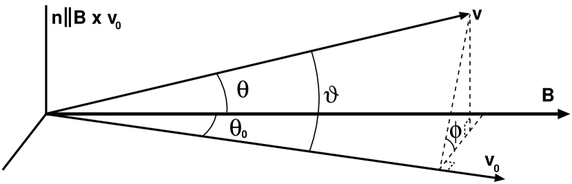
Figure 11: The geometry of the scattering event. Particle is initially moving at velocity $\mathbf{v}_{0}$; the angle between the velocity and magnetic field $\mathbf{B}$ is $\theta_{0}$. (Thus, $\theta_{0}=\arccos\mu_{0}^{\prime}$.) Scattering changes the direction of the particle by an angle $\vartheta$ so that the new velocity $\mathbf{v}$ has an angle $\theta$ between it and the magnetic field. $\phi$ is the azimuth angle of the new velocity measured from the plane defined by $\mathbf{B}$ and $\mathbf{v}_{0}$.

References

- Achterberg et al. (2001) Achterberg, A., Gallant, Y. A., Kirk, J. G., & Guthmann, A. W. 2001, MNRAS, 328, 393
- Bednarz & Ostrowski (1998) Bednarz, J., & Ostrowski, M. 1998, Phys. Rev. Lett., 80, 18, 3911
- Campeanu & Schlickeiser (1992) Campeanu, A. & Schlickeiser, R. 1992, A&A, 263, 413
- Drury (1983) Drury, L. O’C. 1983, Rep. Prog. Phys., 46, 973
- Ellison et al. (1990) Ellison, D. C., Jones, F. C., & Reynolds, S. P. 1990, ApJ, 360, 702
- Kirk & Duffy (1999) Kirk, J. G., & Duffy, P. 1999, J.Phys.G, 25, R163
- Kirk et al. (2000) Kirk, J. G, Guthmann, A. W., Gallant, Y. A., & Achterberg, A. 2000, ApJ, 542, 235
- Lemoine & Pelletier (2003) Lemoine, M., & Pelletier, G. 2003, ApJ, 589, L73
- Meisenheimer et al. (1996) Meisenheimer, K., Röser, H.-J., & Schlötelburg, M. 1996, A&A, 307, 61
- Ostrowski & Schlickeiser (1993) Ostrowski, M., Schlickeiser, R. 1993, A&A, 268, 812
- Schlickeiser (1989) Schlickeiser, R. 1989, ApJ, 336, 243
- Schneider & Kirk (1989) Schneider, P., & Kirk, J.G. 1989, A&A, 217, 344
- Türler et al. (2000) Türler, M., Courvoisier, T. J.-L., & Paltani, S. 2000, A&A, 361, 850
- Vainio (2001) Vainio, R. 2001, Proc. Internat. Cosmic Ray Conf., 6, 2054
- Vainio et al. (2000) Vainio, R., Kocharov, L., Laitinen, T., 2000, ApJ, 528, 1015
- Vainio & Schlickeiser (1998) Vainio, R., & Schlickeiser, R. 1998, A&A, 331, 793
- VVS (2003) Vainio, R., Virtanen, J. J. P., & Schlickeiser, R. 2003 (VVS), A&A, 409, 821
- Valtaoja et al. (1988) Valtaoja, E., et al. 1988, A&A, 203, 1
- Virtanen & Vainio (2003a) Virtanen J., & Vainio R. 2003 (a), in ASP Conf. Proc. 299, High Energy Blazar Astronomy, ed. Takalo, L. O., & Valtaoja, E., 143
- Virtanen & Vainio (2003b) Virtanen J. J. P., & Vainio R. 2003 (b), in The 28:th International Cosmic Ray Conference, OG 1.4, 2023