Frequency ratio method for seismic modeling of $\gamma$ Doradus stars

A method for obtaining asteroseismological information of a $\gamma$ Doradus oscillating star showing at least three pulsation frequencies is presented. This method is based on a first-order asymptotic g-mode expression, in agreement with the internal structure of $\gamma$ Doradus stars. The information obtained is twofold: 1) a possible identification of the radial order $n$ and degree $\ell$ of observed frequencies (assuming that these have the same $\ell$), and 2) an estimate of the integral of the buoyancy frequency (Brunt-Väisälä) weighted over the stellar radius along the radiative zone. The accuracy of the method as well as its theoretical consistency are also discussed for a typical $\gamma$ Doradus stellar model. Finally, the frequency ratios method has been tested with observed frequencies of the $\gamma$ Doradus star HD 12901. The number of representative models verifying the complete set of constraints (the location in the HR diagram, the Brunt-Väisälä frequency integral, the observed metallicity and frequencies and a reliable identification of $n$ and $\ell$) is drastically reduced to six.

1 Introduction

The asymptotic approximation for the solution of linear, isentropic $g$-mode oscillations of high radial order was firstly attempted by Smeyers (1968), Tassoul & Tassoul (1968) and Zahn (1970). These initial approaches were developed for the special case of a star with a convective core and a radiative envelope. From these first developments until recently, all asymptotic solutions have been carried out by using the Cowling (1941) approximation, where the perturbation of the gravitational potential is neglected.

Tassoul (1980) investigated the asymptotic representation of high-frequency $p$-modes and low-frequency $g$-modes associated with low-degree spherical harmonics. There, the procedure of Iweins & Smeyers (1968) and Vandakurov (1967) was adopted to avoid the difficulties of the so-called mobile singularities. This procedure solves different equations in different regions of the star and gives asymptotic expressions for the $p$ and $g$-modes for different stellar structures. Later, Smeyers & Tassoul (1987) used pulsating second-order differential equations, expressed in a single dependent variable, to make the construction of successive asymptotic approximations more transparent.

Tassoul (1990) developed, for the first time, an asymptotic expression for high-frequency non-radial $p$ modes without neglecting the Eulerian perturbation of the gravitational potential. This study was carried out for low-frequency $g$-modes by Smeyers et al. (1995) by using a different asymptotic approach. They applied a procedure described by Kevorkian & Cole (1981) to a fully radiative star, which was extended to a convective core plus a radiative envelope by Willems, Van Hoolst & Smeyers (1997). Since the work of Tassoul (1980), subsequent studies have improved the second order and the eigenfunction descriptions, but the first order asymptotic expressions for the frequency in different physical situations was correctly obtained by Tassoul (1980).

The first attempt to obtain information on a real star by using these $g$-mode asymptotic developments was carried out by Provost & Berthomieu (1986) adapting the second order asymptotic theory of Tassoul (1980) to the special case of the Sun. They argued that the study of the $g$ modes of a star would provide information about the physical conditions of the stellar core. At the same time, Kawaler (1987) and Kawaler & Bradley (1994) started to investigate the internal structure of the PG 1159 hot white dwarf stars through the same asymptotic $g$-mode theory. By using the fully radiative star expression, they obtained stellar properties comparing mode differences of consecutive orders.

Recently, $\gamma$ Doradus stars have been defined by Kaye et al. (1999) as a class of stars pulsating in high-$n$, low-$\ell$ $g$ modes with very low photometric amplitude, lying on or just to the right of the cold border at the lower part of the Cepheid instability strip. During recent years, tens of candidate $\gamma$ Doradus stars have been observed and cataloged (Mathias et al., 2004; Martín, Bossi & Zerbi, 2003, and references therein). Also, several theoretical studies have been carried out to understand their instability mechanism, since the $\kappa$-mechanism does not explain the observed modes (see Guzik et al., 2000; Grigahcène et al., 2004; Dupret et al., 2004).

Modelling these and other pulsating stars is mainly dependent on the fundamental stellar parameters such as metallicity, effective temperature, luminosity and surface gravity as deduced from observations. In the case of the well-known five minute solar oscillations, helioseismology has provided important improvements to our knowledge of the internal structure and evolution of the Sun thanks to the asymptotic theory applied to solar $p$ modes (Christensen-Dalsgaard, Thompson & Gough, 1989), useful for constraining the mass and the evolutionary stage of solar-like pulsating stars by using the $(\Delta\sigma_{0},D_{0})$ diagrams. $\Delta\sigma_{0}$ represents the average separation between modes of the same degree and adjacent radial order and $D_{0}$ is related to the small separation between $\sigma_{n,\ell}$ and $\sigma_{n-1,\ell+2}$. This increases the set of parameters ${\cal P}$ provided by classical observables with the seismic information

$${\cal P}={\cal P}(Z,g,L,{\mathrm{T}_{\mathrm{eff}}};\Delta\sigma_{0},D_{0}).$$

where $Z$ represent the relative metal abundance, $g$ the gravity, $L$ the luminosity and ${\mathrm{T}_{\mathrm{eff}}}$ the effective temperature of the star.

An analogous method for low frequency asymptotic $g$-mode pulsators, such as $\gamma$ Doradus stars, will be given here. Additional constraints can be obtained by using information inferred from ratios of the observed frequencies. Similarly to acoustic modes in the asymptotic regime, our method increases the set of parameters ${\cal P}$ provided by classical observables by

$${\cal P}={\cal P}(Z,g,L,{\mathrm{T}_{\mathrm{eff}}};\frac{f_{o,i}}{f_{o,j}},{\cal I}).$$

where $f_{o,i}$ and $f_{o,j}$ represent the observed frequencies and ${\cal I}$ is the integral of the Brunt-Väisälä frequency defined below. Particularly, this procedure will provide an estimate of the radial and spherical orders $(n,\ell)$ of at least three observed frequencies of a $\gamma$ Doradus star. In addition, the internal stellar structure will also be constrained through the knowledge of the integral along the stellar radius of the Brunt-Väisälä frequency.

The paper is organized as follows: In Sec. 2, the first order analytical asymptotic equation to be used is presented, as well as the physical reasons for the choice of this expression. In Sec. 3, the procedure and a test of its theoretical consistency is discussed. An application of the method to observations of the $\gamma$ Doradus star HD 12901 is given in Sec. 4.

2 Analytical equation for asymptotic $g$ modes

$\gamma$ Doradus stars are found to pulsate in the low frequency g-mode asymptotic regime. There are several analytical forms for obtaining the numerical value of the pulsational period as a function of the radial order $n$, the spherical order $\ell$, different constants and equilibrium quantities, all of them having slight differences and are applied to different internal stellar structures.

Figure 1: Propagation diagram for the theoretical model presented in Table 1. Angular frequencies are given in nondimentional units. The horizontal line represent a standard $\gamma$ Doradus frequency, around $20\,\mu Hz$ ($\omega^{2}$= 0.0018).

These stars present a convective core, a radiative envelope and a small outer convective zone close to the photosphere. The distribution of convective and radiative zones inside the star produces different propagation cavities, which is the key for solving the problem of interpreting the behavior of their $g$-modes in the asymptotic regime. The so-called turning points represent the limits of such cavities. They are defined, depending on the authors, by the zeros of the Brunt–V is l  frequency (Tassoul, 1980) or by the points of intersection of the propagating mode with the Brunt–V is l  and Lamb frequencies, whichever comes first (Shibahashi, 1979) (see Fig. 1). Both quantities represent the characteristic buoyancy (Brunt–V is l ) and acoustic (Lamb) frequencies (Unno et al., 1989).

For the $\gamma$ Doradus internal distribution of convective and radiative zones, the better adapted analytical solution is

$$\sigma^{a}_{n,\ell}\approx\frac{[\ell(\ell+1)]^{1/2}}{(n+1/2)\pi}{\cal I}$$ (1)

given by Tassoul (1980) and obtained under the assumption of adiabaticity and non-rotation. $\cal I$ is the integral of the Brunt-Väisälä frequency, given by

$${\cal I}=\int_{r_{a}}^{r_{b}}\frac{N}{r}\mathrm{d}r\leavevmode\nobreak\ ,$$ (2)

where $r_{a}$ and $r_{b}$ represent the inner and outer turning points respectively.

Considering low $g$-mode frequencies in the asymptotic regime (typical of $\gamma$ Doradus stars), the inner turning point ($r_{a}$) is clearly defined by the zero of $N^{2}$ (Fig. 1). However, for the outer layers, small changes in the frequency produce different turning points ($r_{b}$) depending on whether the frequency intersects first $N^{2}$ or $L^{2}_{2}$ (see Fig. 1) compared to the zero of $N^{2}$. The problem of considering one of these possibilities remains unsolved. This theoretical question beyond the scope of the present work, however an estimate of the error committed when considering Eq. 1 can be calculated. To do so, theoretical oscillation frequencies $\sigma_{n,\ell}$ computed from a given model (see Table 1) are compared with those obtained from Eq. 1. Such errors, defined as

$$\epsilon_{r,\sigma}=\Big{|}\frac{\sigma_{n,\ell}-\sigma^{a}_{n,\ell}}{\sigma_{n,\ell}}\Big{|},$$ (3)

are shown in Fig. 2 for $\ell\!\!=\!1$ and $\ell=2$ modes. As expected, $\epsilon_{r,\sigma}$ increases with the mode frequency and hence decreases with $n$, since they depart from the asymptotic regime. In the range of frequencies in which $\gamma$ Doradus stars pulsate, these errors remain around 1–2%.

Equivalently, the relative error committed when calculating ${\cal I}$ values from Eq. 1 can be investigated through

$$\epsilon_{r,{\cal I}}=\Big{|}\frac{{\cal I}_{\mathrm{th}}-{\cal I}^{a}_{i}}{{\cal I}_{\mathrm{th}}}\Big{|},$$ (4)

where ${\cal I}^{a}_{i}$ is calculated for each mode provided the frequency and the radial and spherical orders of the modes, and ${\cal I}_{\mathrm{th}}$ represents the integral ${\cal I}$ calculated for the theoretical model. Errors obtained in this case are of the same order as $\epsilon_{r,\sigma}$, and the average value of $1\%$ observed in Fig. 2 will be used in Sec. 4. They remain lower than typical errors given by the resolution of observed frequencies and hence, of their ratios. This represents an important advantage for the method since no significant additional uncertainties need to be considered besides those coming from observations.

Therefore, considering all previous arguments, the analytic form (Eq. 1) given by Tassoul (1980) will be adopted in this work.

Figure 2: Relative errors of asymptotic frequencies compared to theoretical predictions ($\epsilon_{r,\sigma}$) by using Eq. 1 for a complete theoretical oscillation spectrum. See text for details.

3 Frequency Ratio method

3.1 Method bases

In the case of asymptotic acoustic modes, physical information can be inferred from frequency differences of adjacent radial order modes. This can be done since the model dependence appears in the equation as an adding term. As can be seen from the analytic form for asymptotic $g$ modes (Eq. 1), it is not possible to retrieve physical information from frequency differences. However, the role played by such frequency differences can be replaced by frequency ratios.

Let us consider two modes $\sigma_{\alpha_{1}}$ and $\sigma_{\alpha_{2}}$, with $\alpha_{1}\equiv({n_{1}},{\ell_{1}})$ and $\alpha_{2}\equiv({n_{2}},{\ell_{2}})$ respectively. For sake the of simplicity, the same mode degree $\ell_{1}=\ell_{2}=\ell$ of a non-rotating pulsating star, showing adiabatic $g$ modes in asymptotic regime, is considered. Their eigenfrequencies can be approximated by Eq. 1 which is model-dependent through the integral given by Eq. 2. As shown in Fig. 1, for typical $\gamma$ Doradus frequency ranges, the possible slight differences of the outer turning point location can be considered negligible as far as the calculation of ${\cal I}$ is concerned. It can thus be approximated as constant (${\cal I}_{\alpha_{2}}={\cal I}_{\alpha_{1}}={\cal I}$), and therefore, the ratio of $\sigma_{\alpha_{1}}$ and $\sigma_{\alpha_{2}}$ can be approximated by

$$\frac{\sigma_{\alpha_{1}}}{\sigma_{\alpha_{2}}}\approx\frac{n_{2}+1/2}{n_{1}+1/2}\;\;.$$ (5)

An estimate of the radial order ratios of these frequencies can thus be obtained. A value of the integral can also be deduced from observations ${\cal I}_{obs}$, provided that an estimate of the mode degree $\ell$ is assumed. Constraints on models will come from the consistency of: 1) the radial order identification corresponding to the observed ratios; 2) their corresponding order $\ell$ and 3) the observed Brunt–V is l  integral.

On the other hand, the assumption of equal $\ell$ for all the observed modes is not imperative for this procedure. Additional information on $\ell$ provided by spectroscopy or multicolor photometry can be exploited through the following expression (see Tassoul, 1980)

$$\frac{\sigma_{{n_{1}},{\ell_{1}}}}{\sigma_{{n_{2}},{\ell_{2}}}}\approx\frac{n_{2}+1/2}{n_{1}+1/2}\frac{\sqrt{\ell_{1}(\ell_{1}+1)}}{\sqrt{\ell_{2}(\ell_{2}+1)}}$$ (6)

which is the extended form of Eq. 5.

The efficiency and utility of this method depend on the number of observed frequencies N_f. The larger N_f, the lower the number of integers verifying Eq. 5. The method becomes useful for N${}_{f}\geq 3$.

3.2 Theoretical test

To test the self-consistency of this technique, consider a theoretical numerical simulation of a given star. Assuming three theoretical frequencies computed for a $1.5{\mathrm{M}_{\odot}}$ typical $\gamma$ Doradus model on the Main Sequence, the ratio method is applied to obtain an estimate of the radial order $n$ and the spherical order $\ell$ of these frequencies as well as their corresponding ${\cal I}$. If this procedure is self-coherent, at least one of all possible solutions will correspond to the selected theoretical frequencies and the corresponding ${\cal I}$ value.

Table 1: $\ell$, $n$ and frequency $\sigma$ in $\mu Hz$ for a complete spectrum of the theoretical model displayed at the top of the table.

$\log\,{\mathrm{T}_{\mathrm{eff}}}$	$\log\,g$	$\log\frac{L}{L_{\odot}}$	$X_{c}$	$\frac{M}{M_{\odot}}$	${\cal I}_{\mathrm{th}}$
3.845	4.045	0.873	0.29	1.5	839
$\ell$	$n$	$\sigma$ $(\mu Hz)$	$\ell$	$n$	$\sigma$ $(\mu Hz)$
1	30	12.3052	1	22	16.6262
1	29	12.7176	1	21	17.4038
1	28	13.1589	1	20	18.2397
1	27	13.6375	1	19	19.1344
1	26	14.1553	1	18	20.1369
1	25	14.7063	1	17	21.2964
1	24	15.2893	1	16	22.6059
1	23	15.9219	1	15	24.0274
2	53	12.1277	2	40	16.0399
2	52	12.3621	2	39	16.4502
2	51	12.5999	2	38	16.8789
2	50	12.8444	2	37	17.3283
2	49	13.1012	2	36	17.8010
2	48	13.3737	2	35	18.2982
2	47	13.6612	2	34	18.8212
2	46	13.9616	2	33	19.3752
2	45	14.2724	2	32	19.9675
2	44	14.5931	2	31	20.6010
2	43	14.9264	2	30	21.2734
2	42	15.2772	2	29	21.9839
2	41	15.6484	2	28	22.7434

The theoretical eigenfrequencies (computed by the code FILOU, see Sec. 4.2) of a typical $\gamma$ Doradus model, as well as its ${\cal I}_{th}$ value in $\mu Hz$ are given in Table 1.

A first test of the ratio method is carried out for three close $\ell=1$ modes, for instance $(n,\sigma)=(25,14.706)$, $(23,15.922)$ and $(20,18.240)$. The corresponding frequency ratios are

$$\frac{\sigma_{1}}{\sigma_{2}}=0.9236,\leavevmode\nobreak\ \leavevmode\nobreak\ \frac{\sigma_{2}}{\sigma_{3}}=0.8729,\leavevmode\nobreak\ \leavevmode\nobreak\ \frac{\sigma_{1}}{\sigma_{3}}=0.8063$$ (7)

which constitute our assumed observed frequency ratios. As in this theoretical test the radial order of selected frequencies is known, it is possible to study the accuracy of Eq. 5 by comparing the corresponding $n$ ratios:

$$\frac{n_{2}+1/2}{n_{1}+1/2}=\beta_{1}=0.9216,\leavevmode\nobreak\ \leavevmode\nobreak\ \beta_{2}=0.8723,\leavevmode\nobreak\ \leavevmode\nobreak\ \beta_{3}=0.8039$$ (8)

yielding an error of $2\times 10^{-3}$, $6\times 10^{-4}$ and $24\times 10^{-4}$ respectively. In Fig. 3, the accuracy of Eq. 5, defined as

$$\epsilon_{\beta}=\frac{\sigma_{i}}{\sigma_{j}}-\frac{n_{j}+1/2}{n_{i}+1/2}$$ (9)

is shown for all the frequencies of Table 1. The maximum departure of the $n$ ratio from the real frequency ratios is $5\cdot 10^{-3}$, allowing us to consider this value as the error when applying this method.

Figure 3: Error $\epsilon_{\beta}$ between the frequency ratios and the corresponding asymptotic predictions, for the complete spectrum of the theoretical model.

3.2.1 Radial order identification

If the values of the radial orders are assumed unknown and their errors are supposed to be given by the maximum of $\epsilon_{\beta}$ (Eq. 9), i.e. $5\cdot 10^{-3}$, ratios of integer numbers are searched for within the following ranges

$$\frac{\sigma_{1}}{\sigma_{2}}=[0.929,0.919]$$

$$\frac{\sigma_{2}}{\sigma_{3}}=[0.878,0.868]$$ (10)

$$\frac{\sigma_{1}}{\sigma_{3}}=[0.811,0.801]$$

Integer numbers contemplated here (from 1 to 60) cover the range of typical $g$-mode radial orders shown by $\gamma$ Doradus stars. Within this range, there exist several possible integer numbers yielding the same value for each ratio of Eq. 10. However, the key point consists of searching for ($n_{1},n_{2},n_{3}$) sets verifying

$$\frac{n_{2}+0.5}{n_{1}+0.5}\sim\frac{\sigma_{1}}{\sigma_{2}},\leavevmode\nobreak\ \leavevmode\nobreak\ \frac{n_{3}+0.5}{n_{2}+0.5}\sim\frac{\sigma_{2}}{\sigma_{3}},\leavevmode\nobreak\ \leavevmode\nobreak\ \frac{n_{3}+0.5}{n_{1}+0.5}\sim\frac{\sigma_{1}}{\sigma_{3}}$$ (11)

and limiting thus the final number of valid sets.

Table 2: Radial number $n$ for each selected frequency, $\ell$ and Brunt-Väisälä integral (in $\mu$Hz) estimated by the frequency ratio method for the assumed observed frequencies $(20,18.2397)$, $(23,15.9219)$ and $(25,14.7063)$ with $\ell=1$. The real values of the radial and spherical orders are displayed in boldface.

$n_{1}$	$n_{2}$	$n_{3}$	$\ell$	${\cal I}_{\mathrm{th}}$	$\epsilon_{\beta}$
20	23	25	1	831	0.0017
33	38	41	1	1360	-0.0007
33	38	41	2	784	-0.0007
41	47	51	2	971	0.0003
21	24	26	1	702	-0.0035
42	48	52	2	801	-0.0023
34	39	42	1	1127	-0.0039
34	39	42	2	651	-0.0039
40	46	50	2	764	0.0030

Once all possible sets have been obtained, an estimated spherical order $\ell$ to which $n_{1}$, $n_{2}$ and $n_{3}$ are associated can also be identified. To do so, selected sets are compared with theoretical oscillation spectra computed from representative models of $\gamma$ Doradus stars. Finally, for each solution ($\sigma,n,\ell$) found, an estimate of ${\cal I}_{\mathrm{th}}$ (${\cal I}$ is approximately constant within each set) can also be deduced through Eq. 1.

In this exercise seven possible sets have been obtained. The real $n$ and $\ell$ (our simulated observations) have been retrieved (boldface in Table 2) together with other eight possible identifications. In addition, an accurate prediction of the Brunt-Väisälä frequency is also obtained. To investigate other distributions of observed frequencies (always within the asymptotic regime), the following cases are studied: 1) modes with very different radial order, for instance $(n_{1}=16,n_{2}=23,n_{3}=28)$ and $\ell=1$; 2) close consecutive radial orders, for instance $(n_{1}=45,n_{2}=47,n_{3}=50)$ and $\ell=2$; and 3) very different radial orders $(n_{1}=30,n_{2}=45,n_{3}=53)$ and $\ell=2$. Following the same procedure, sets of 6, 5 and 8 possible solutions are obtained. For all of them, the real values of $n$ and $\ell$ (boldface in Table 3), and an estimate of ${\cal I}$ very close to the values from the model are obtained.

These results are very important since they show the self-consistency of the method which, in turn, reduces drastically the number of representative models of a given $\gamma$ Doradus star. Moreover, they illustrate the good accuracy of Eq. 1 for this kind of study.

Table 3: Radial number $n$ for each selected frequency, $\ell$ and Brunt-Väisälä integral estimated by the frequency ratio method for the assumed observed frequencies $(16,22.6059)$, $(23,15.9219)$ and $(28,13.1589)$ with $\ell=1$ (set 1), $(45,14.2724)$, $(47,13.6612)$ and $(50,12.8444)$ with $\ell=2$ (set 2) and $(30,21.2734)$, $(45,14.2724)$ and $(53,12.1277)$ with $\ell=2$ (set 3), See text for details. The real radial and spherical orders are displayed in boldface.

set	$n_{1}$	$n_{2}$	$n_{3}$	$\ell$	${\cal I}_{\mathrm{th}}$	$\epsilon_{\beta}$
1	26	37	45	2	768	-0.0001
	33	47	57	2	971	-0.0004
	16	23	28	1	830	0.0024
	23	33	40	1	1182	0.0013
	23	33	40	2	682	0.0013
	30	43	52	2	886	0.0007
set	$n_{1}$	$n_{2}$	$n_{3}$	$\ell$	${\cal I}_{\mathrm{th}}$	$\epsilon_{\beta}$
2	46	48	51	2	850	-0.0020
	45	47	50	2	832	-0.0007
	43	45	48	2	798	0.0021
	44	46	49	2	815	0.0006
	47	49	52	2	869	-0.0033
set	$n_{1}$	$n_{2}$	$n_{3}$	$\ell$	${\cal I}_{\mathrm{th}}$	$\epsilon_{\beta}$
3	22	33	39	1	1063	0.0005
	22	33	39	2	614	0.0005
	26	39	46	1	1252	0.0001
	26	39	46	2	723	0.0001
	30	45	53	2	833	-0.0004
	34	51	60	2	941	-0.0002
	33	49	58	2	910	-0.0016
	18	27	32	1	876	0.0008

4 An application: The $\gamma$ Doradus star HD 12901

Once the frequency ratio method has been shown to be self-consistent, a test with real data must be carried out for the $\gamma$ Doradus star HD 12901. This star pulsates with three frequencies (Table 4) in the asymptotic regime (see Sec. 3 for more details).

Table 4: Photometric observed frequencies in both cycles per day and ${\mu\mbox{Hz}}$ for the $\gamma$ Doradus star HD 12901, taken from Aerts et al. (2004).

	$\nu$	$\nu$
	($c/d$)	(${\mu\mbox{Hz}}$)
$f_{\rm I}$	1.216	14.069
$f_{\rm II}$	1.396	16.157
$f_{\rm III}$	2.186	25.305

4.1 Fundamental parameters

The fundamental parameters of HD 12901 have been determined by applying TempLogG (Rogers, 1995) to the Strömgren–Crawford photometry listed in the Hauck-Mermilliod catalogue (Hauck & Mermilliod, 1998). In this catalogue, no $\beta$ index value is given for HD 12901, which was instead obtained from Handler (1999). The code classifies this object as a main sequence star in the spectral region F0-G2. The resulting physical parameters are summarized in Table 5.

Table 5: Physical parameters of the stars HD 12901taken from the literature. The values of the rotational velocities are also listed.

HD	${\mathrm{T}_{\mathrm{eff}}}$	${\log\,g}$	${\rm[Fe/H]}$	${v\!\sin\!i}$	Ref.
	(K)	(dex)	(dex)	(km s-1)
12901	6996	4.04	$-0.37$		$a$
	7079	4.47	$-0.40$		$b$
				53	$c$
				66	$d$

$a$: TempLogG (Rogers, 1995)
$b$: Dupret (2002)
$c$: Aerts et al. (2004)
$d$: Mathias et al. (2004)

Dupret (2002) gives also physical parameters for HD 12901 based on the Geneva photometry of Aerts et al. (2004) and the calibrations given by Kunzli et al. (1997) for the Geneva photometry of B to G stars. In his study, theoretical stellar models for this star do not take into account their surface gravity determinations, as they are too high, corresponding to models below the ZAMS.

Values for the ${v\!\sin\!i}$ were taken from Royer et al. (2002), computed from spectra collected at the Haute-Provence Observatory (OHP) and by Aerts et al. (2004), derived from a cross-correlation function analysis of spectroscopic measurements with the CORALIE spectrograph. Mathias et al. (2004) have published the results of a two-year high-resolution spectroscopic campaign, monitoring 59 $\gamma$ Doradus candidates. In this campaign, more than 60% of the stars presented line profile variations which can be interpreted as due to pulsation. From this work, in which projected rotational velocities were derived for all 59 candidates, an additional value of ${v\!\sin\!i}$ is obtained for HD 12901.

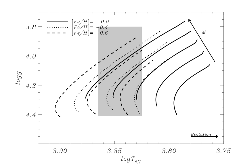
Figure 4: Evolutionary tracks of models representative of HD 12901 in a $g$–${\mathrm{T}_{\mathrm{eff}}}$ (in a logarithmic scale). The shaded area represents the observational error box as deduced from Table 5. From bottom to top, masses of models vary from 1.2 to $1.6{\mathrm{M}_{\odot}}$. Continuous lines represent evolutionary tracks of models computed with [Fe/H]=0.0 (the solar value). Dotted lines represent those computed with [Fe/H]=-0.4 and dashed lines are those computed with [Fe/H]=-0.6.

The physical parameters used in the present work to delimit the error boxes for the star in the HR diagram are those given by TempLogG, derived from the Strömgren–Crawford photometry and given in blold font in Table 5. Errors for these parameters will be assumed to be approximately $0.2$ dex in ${\log\,g}$ and $200$ K in ${\mathrm{T}_{\mathrm{eff}}}$.

4.2 Modelling

The evolutionary code CESAM (Morel, 1997) has been used to compute stellar equilibrium models. The physics have been chosen as adequate for intermediate mass stars. Particularly, the opacity tables are taken from the OPAL package (Iglesias & Rogers, 1996), complemented at low temperatures ($T\leq 10^{3}\,K$) by the tables provided by Alexander & Ferguson (1994). The convective transport is described by the classical ML theory, in which the free parameters $\alpha_{ML}=l_{m}/\mathrm{H}p=1.8$ and a mixed core overshooting parameter $d_{ov}=l_{ov}/\mathrm{H}p=0.2$ are considered (as prescribed by Schaller et al., 1992, for intermediate mass stars). The $\mathrm{H}p$ corresponds to the local pressure scale-height. $l_{m}$ and $d_{ov}$ represent the mixing length and the inertial penetration distance of convective bulbs respectively. For the atmosphere reconstruction, Eddington’s $T(\tau)$ law (grey approximation) is used. The transformation from heavy element abundances with respect to hydrogen [M/H] into concentration in mass $Z$ assumes an enrichment ratio of $\Delta Y/\Delta Z=2$ and $Y_{\mathrm{pr}}=0.235$ and $Z_{\mathrm{pr}}=0$ as helium and heavy element primordial concentrations.

To cover observational errors in the determination of ${\mathrm{T}_{\mathrm{eff}}}$, ${\log\,g}$ and [Fe/H], equilibrium models are computed within a mass range of 1.2–$1.6{\mathrm{M}_{\odot}}$ and metallicities from -0.6 up to the solar value (Fig. 4). Theoretical oscillation spectra are computed with the oscillation code FILOU (see Tran Minh & L on, 1995; Suárez, 2002). Eigenfrequencies are computed for mode degree values of up to $\ell=2$, thus covering the range of observed $g$ modes for $\gamma$ Doradus stars (up to $g_{60}$).

4.3 Locating HD 12901 in a ${\cal I}$ – $\log{\mathrm{T}_{\mathrm{eff}}}$ diagram

4.3.1 Observed frequency ratios

Following the steps described in Sec. 3, the ratios of observed frequencies are:

$$\frac{f_{\rm I}}{f_{\rm II}}=0.871,\leavevmode\nobreak\ \leavevmode\nobreak\ \frac{f_{\rm II}}{f_{\rm III}}=0.639,\leavevmode\nobreak\ \leavevmode\nobreak\ \frac{f_{\rm I}}{f_{\rm III}}=0.556.$$ (12)

On the other hand, all possible integer number ratios up to $n=60$ are calculated. An error of $5\cdot 10^{-3}$ on ratios values is assumed in order to match the theoretical uncertainties found in Fig. 3. With these assumptions and considering only dipoles ($\ell=1$) and quadrupoles ($\ell=2$), as has usually been found in this type of star, all possible sets ($\sim 60$) were reduced to six, given in Table 6. For each set, the spherical order $\ell$ is estimated by comparing their radial orders with theoretical spectra for representative models (see Sec. 4.2 and Table. 1). Furthermore, it is possible to obtain the observed Brunt–V is l  integral (${\cal I}_{obs}$) through Eq. 1, constituting one of the main constraints of this method.

Table 6: List of selected integer numbers sets associated to the observed frequency ratios of HD 12901. For each set, the corresponding observed ${\cal I}_{obs}$ is given in ${\mu\mbox{Hz}}$. An estimate of the spherical order $\ell$ is given in column 4.

	$n_{1}$	$n_{2}$	$n_{3}$	$\ell$	${\cal I}_{\mathrm{obs}}$
$t_{1}$	17	27	31	1	987.0
$t_{2}$	21	33	38	1	1202.4
$t_{3}$	21	33	38	2	694.2
$t_{4}$	26	41	47	2	860.0
$t_{5}$	30	47	54	2	984.3
$t_{6}$	33	52	60	2	1087.9

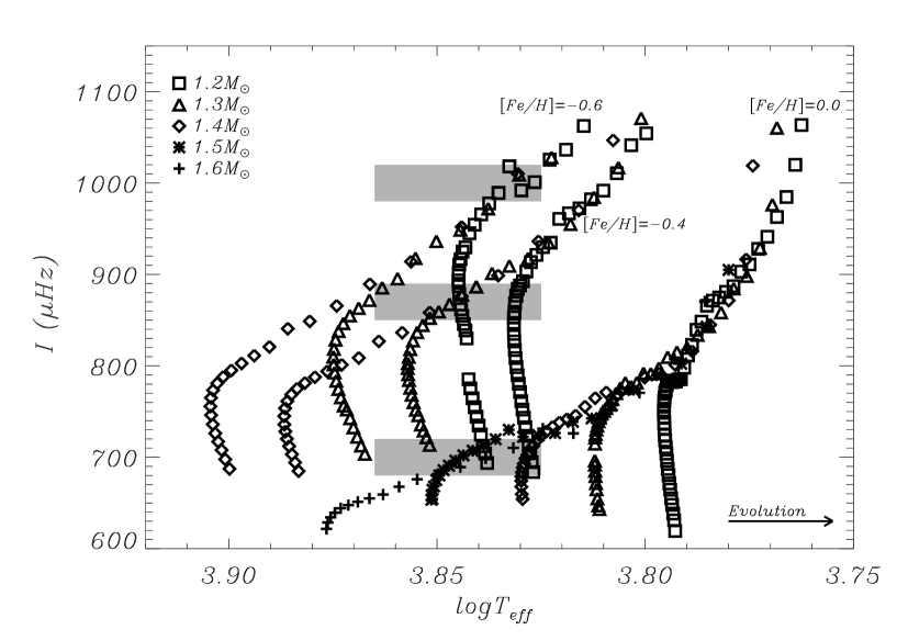
Figure 5: $\cal I$ as a function of the effective temperature for representative models of HD 12901with masses in the range of $M=1.2$–1.6${\mathrm{M}_{\odot}}$, for three different metallicities $[Fe/H]=$0.0, -0.4 and -0.6. Shaded areas represent uncertainty (${\cal I}_{\mathrm{obs}}$,$\log{\mathrm{T}_{\mathrm{eff}}}$) boxes of selected sets $t_{1}$, $t_{3}$ and $t_{4}$ as given in Table 6.

4.3.2 The ${\cal I}$–$\log{\mathrm{T}_{\mathrm{eff}}}$ diagram

For each valid set of integer numbers ($t_{i}$ in Table 6) there is only one associated ${\cal I}_{obs}$ value, as deduced from Eq. 1. Selected ${\cal I}_{\mathrm{obs}}$ can thus be located on a theoretical ${\cal I}$–$\log{\mathrm{T}_{\mathrm{eff}}}$ diagram. This is done in Fig. 5 for the selected $t_{i}$. Only $t_{1}$, $t_{3}$ and $t_{4}$ are displayed since $t_{2}$ and $t_{6}$ give a Brunt–V is l  integral value impossible to reproduce with the theoretical models (see Fig. 5), and $t_{5}$ has a ${\cal I}_{obs}$ impossible to differentiate from $t_{1}$ in the ${\cal I}$–$\log{\mathrm{T}_{\mathrm{eff}}}$ diagram. The theoretical ${\cal I}$ is computed for a set of representative models of HD 12901 (Fig. 4) in the range of 1.2–$1.6{\mathrm{M}_{\odot}}$ for three different metallicities ([Fe/H]= 0.0, $-0.4$ and $-0.6$).

Models are computed within an error box that takes into consideration the typical accuracy for the calculation of physical parameters. As discussed in Sec. 2, a numerical uncertainty in ${\cal I}$ of 1% is chosen.

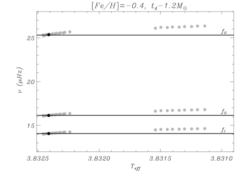
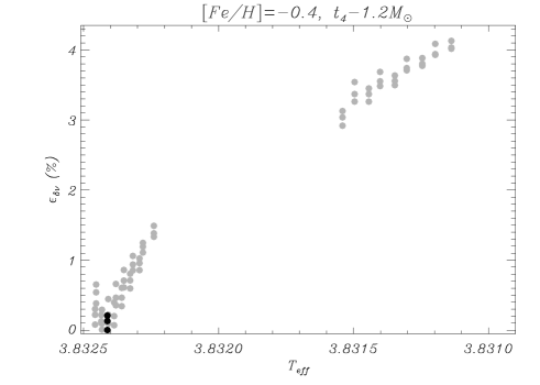
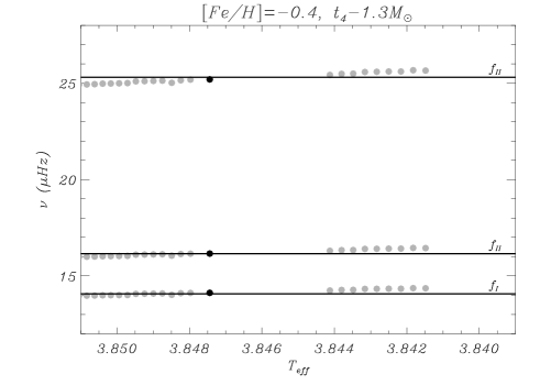
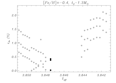
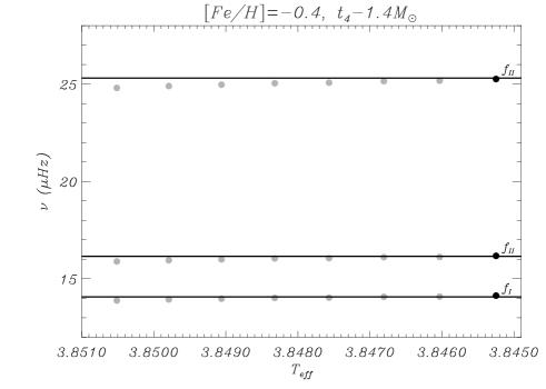
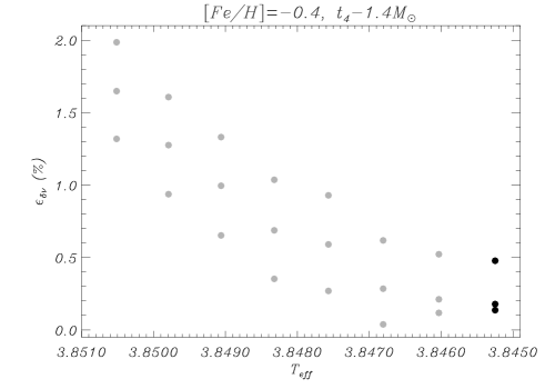
Figure 6: Evolution of theoretical frequencies (left panels) ($g_{26}$,$g_{41}$,$g_{47}$;$\ell=2$) corresponding to the set $t_{4}$ (see Table 6) for selected $1.2$, $1.3$ and $1.4{\mathrm{M}_{\odot}}$ models with a metallicity of [Fe/H]=-0.4 and ${\cal I}_{th}={\cal I}_{obs}(t_{4})$. Filled circles represent such frequencies for each model within the photometric error box of Fig. 4. The observed frequencies $f_{\mathrm{I}}$, $f_{\mathrm{II}}$ and $f_{\mathrm{III}}$ are represented by continuous lines. Right panels show the error $\epsilon_{\delta\nu}$ of theoretical frequencies with respect to the observed ones for each panel on the left. Frequencies of best models are represented by black circles.

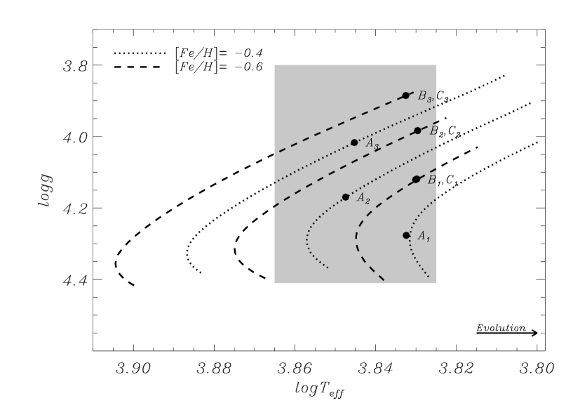
Figure 7: Surface gravity as a function of the effective temperature of seleceted best models following the procedure given in Fig. 6. These selected models are represented by filled circles which are labeled in Table 7. Evolutionary tracks of concerned models are also displayed: as in Fig.4, dotted lines represents tracks for models with [Fe/H]=-0.4 and dashed lines those for models with [Fe/H]=-0.6. The shaded area represents the observational error box deduced from Table 5.

Table 7: Charateristics of the selected best models obtained by comparing theoretical frequencies of deduced sets from representative models with ${\cal I}_{th}\approx{\cal I}_{obs}$. Effective temperatures and luminosities are given on a logarithmic scale. Ages are given in Myr. For each selected model, the corresponding mode degree $\ell$ is also given.

	$\ell$	[Fe/H]	M$/{\mathrm{M}_{\odot}}$	${\mathrm{T}_{\mathrm{eff}}}$	L$/{\mathrm{L}_{\odot}}$	$\log\,g$	$X_{c}$	Age	${\bar{\rho}}/{\bar{\rho}}_{\odot}$
$A_{1}$	2	-0.4	1.2	3.83	0.52	4.28	0.50	1990	9.19
$A_{2}$	2	-0.4	1.3	3.85	0.72	4.17	0.40	2100	6.10
$A_{3}$	2	-0.4	1.4	3.84	0.90	4.02	0.26	2090	3.47
$B_{1}$, $C_{1}$	1,2	-0.6	1.2	3.83	0.67	4.12	0.27	3120	5.36
$B_{2}$, $C_{2}$	1,2	-0.6	1.3	3.83	0.84	3.98	0.17	2720	3.20
$B_{3}$, $C_{3}$	1,2	-0.6	1.4	3.83	0.98	3.88	0.10	2290	2.20

4.4 Toward the modal identification

At this stage, the choice of good models is drastically reduced to those within the ${\cal I}_{\mathrm{obs}}$–$\log{\mathrm{T}_{\mathrm{eff}}}$ boxes obtained for each $t_{i}$ set given in Table 6. Nevertheless it is possible to provide further constraints on both equilibrium models and modal identification from additional observational information.

Considering the observed metallicity for HD 12901 (see Table 5) and the corresponding error in its determination, only models with [Fe/H]=$-0.4$ and $-0.6$ are kept. This reduces the set of possible valid identifications to $t_{1}$, $t_{4}$ and $t_{5}$ with their corresponding spherical order, $\ell$ and ${\cal I}_{\mathrm{obs}}$ values, shown in Table 6. This constrains the mass of models to the range of 1.2–1.4${\mathrm{M}_{\odot}}$.

4.4.1 Theoretical frequencies

Another constraint for selecting the theoretical models fitting the observations consists of comparing, for each set, the theoretical frequencies corresponding to each $n_{i}$ with the observed frequencies. To do so, theoretical oscillation spectra have been computed in the range of $g$ modes given by selected $t_{1}$, $t_{4}$ and $t_{5}$ sets for models within the error (shaded) boxes of Fig. 5.

In Fig. 6, the set of models verifing the integral value of $t_{4}$ is depicted. All these models have thus a metallicity of $-0.4$. From top to bottom different masses are shown ($1.2$, $1.3$ and $1.4M_{\odot}$). In left panels the frequencies for the modes $g_{26}$, $g_{41}$ and $g_{47}$ (see chain $t_{4}$) obtained with each model are represented. The horizontal lines are the observed frequencies of HD 12901. From these panels it becomes apparent that there is a model verifing fairly well the complete chain obtained by our method as well as the observed physical characteristics. The right panels show the relative error defined as follows:

$$\epsilon_{\delta\nu}=\Big{|}\frac{\nu_{i}-\nu_{obs}}{\nu_{obs}}\Big{|}$$ (13)

The choice of the best model within a track can be carried out by searching for the model minimizing this relative error. This model is represented in Fig. 6 by filled circles. Repeating this procedure for the rest of the selected models in Fig. 5 it is possible to restrict the complete sets of models to just nine. Seismic models with the same mass and metallicity but verifing modal identifications with different $\ell$ are computed from the same equilibrium model. This reduces the total number of theoretical models fitting HD 12901 to 6 (those verifing the complete constraints concerning $\log{\mathrm{T}_{\mathrm{eff}}}$, $\log g$, metallicity, $(n,l,\sigma)$ and $\cal I_{obs}$ for each observed frequency). In Table 7 the charateristics of the selected best models are displayed.

This final set of models is depicted in the HR diagram in Fig. 9. As can be seen in Table 7, this set is very heterogeneous, with very different hydrogen central concentration, age, $\log g$ and/or mean density. This is particularly useful when additional constraints on models exist. In this context, information on the spherical degree of modes (from multicolour photometry (Moya et al., 2004) or spectroscopy) would be specially helpful in discriminating between models. In particular, in Aerts et al. (2004), the three frequencies of HD 12901 are suggested to be $\ell=1$. This would restrict the representative models of the star to $B_{1}$, $B_{2}$ and $B_{3}$.

Further constraints from the pulsational behaviour of $\gamma$ Doradus stars are likely to complete the method presented here. Particularly, constraints on unstable modes considering a convection–pulsation interaction can be obtained (work in preparation) from recent theoretical developments of Grigahcène et al. (2004) and Dupret et al. (2004).

5 Conclusions

By using the first order asymptotic representation for the low-frequency g-mode eigenvalues of stellar pulsations, a method for estimating the radial and spherical orders as well as the Brunt–V is l  integral is presented. The method is developed under the assumptions of adiabaticity and no rotation, and is based on information gathered from ratios of observed frequencies, similary to the large and small frequency difference for high-order $p$ modes. It can be shown that the method becomes useful when applied to at least 3 frequencies. For each of these observed frequencies, some information about the $\ell$ of each mode or the assumption that all of them have the same $\ell$ is needed.

The frequency method is specially adapted to $\gamma$ Doradus stars for two main reasons: 1) they oscillate with $g$ modes in the asymptotic regime and 2) their internal structure (a radiative envelope between two convective zones, the inner core and other close to the photosphere) make it possible to use an asymptotic expression with only one scaling model-dependent parameter, the Brunt–V is l  integral.

The self-consistency of this method is verified by means of a theoretical exercise in which the accuracy of predictions given by the expresion obtained by Tassoul (1980) for asymptotic $g$ modes is checked. These predictions are compared with theoretical frequencies computed for a model representative of a typical $\gamma$ Doradus star.

An application to the real star HD 12901 is also given. This star has been recently found to be a $\gamma$ Doradus star and three oscillation frequencies have been identified (Aerts et al., 2004). Nine possible mode identifications ($n$,$\ell$) as well as the corresponding Brunt–V is l  integral estimates are obtained. From standard constraints on models coming from fundamental parameters (mainly ${\log\,g}$, ${\mathrm{T}_{\mathrm{eff}}}$ and metallicity), nine sets of representative models are selected. From these models, theoretical frequencies computed for the nine mode identifications obtained are compared with observations. This lowers the total number of representative models of HD 12901 to six. Furthermore, recent multicolor photometry results for this star given by Aerts et al. (2004) suggest the spherical order to be $\ell=1$. This drastically reduces the number of valid models fitting the observations to only three.

This method constitutes an important step toward the modal identification of $\gamma$ Doradus stars, especially in cases when there is no additional information, like that provided by multicolour photometry or high resolution espectroscopy. It is, therefore, a method well suited for the particular case of the white-light, very high precision photometry expected to be delivered by the asteroseismology camera of the COROT mission (Baglin & Auvergne, 1997). Nevertheless, improvements coming from the pulsational behaviour of $\gamma$ Doradus stars  such as unstable mode predictions considering a convection–pulsation interaction, and additional spectroscopy or multicolor photometry information will complete the method here presented. Therefore, this method, together with the additional information mentioned above, represents a complete scheme for studying and interpreting the observational behaviour of $\gamma$ Doradus stars.