Extended Source Effects in Substructure Lensing

Abstract

We investigate the extended source size effects on gravitational lensing in which a lens consists of a smooth potential and small mass clumps (“substructure lensing”). We first consider a lens model that consists of a clump modeled as a singular isothermal sphere (SIS) and a primary lens modeled as an external background shear and convergence. For this simple model, we derive analytic formulae for (de)magnification of circularly symmetric top-hat sources with three types of parity for their lensed images, namely, positive, negative, and doubly negative parities. Provided that the source size is sufficiently larger than the Einstein radius of the SIS, we find that in the positive (doubly negative) parity case, an extended source is always magnified (demagnified) in comparison with the unperturbed macrolens system, whereas in the negative parity case, the (de)magnification effect, which depends on the sign of convergence minus unity is weaker than those in other parities. It is shown that a measurement of the distortion pattern in a multiply lensed image enables us to break the degeneracy between the lensing effects of clump mass and those of clump distance if lensing parameters of the relevant macrolens model are determined from the position and flux of multiple images. We also show that an actual density profile of a clump can be directly measured by analyzing the “fine structure” in a multiply lensed image within the Einstein radius of the clump.

1 Introduction

The standard cold dark matter (CDM) scenario predicts the presence of several hundred small-mass clumps or “subhalos” ($\lesssim 10^{8}M_{\odot}$) in a galaxy-sized halo ($\sim 10^{12}M_{\odot}$), while the observed number of dwarf galaxies around the Milky Way is only a dozen (Klypin et al. 1999; Moore et al. 1999). This suggests the presence of several hundred subhalos holding few or no stars around such a galaxy. Gravitationally lensed QSOs with quadruple images have recently been used for putting a limit on the surface density and the mass of such invisible substructures (Mao & Schneider 1998; Metcalf & Madau 2001; Chiba 2002; Metcalf & Zhao 2002; Dalal & Kochanek 2002; Bradac et al. 2002). Statistical analyses on these quadruple QSO-galaxy lensing systems show that the (de)magnification of lensed images and its dependence on their parities can be explained by the presence of substructures along the line of sight to the images, in contrast to the lens models relying on “smooth perturbation” in the gravitational potential of a macrolens (Metcalf & Zhao 2002; Keeton et al. 2002; Evans & Witt 2003).

However, there are two ambiguities in these QSO-galaxy lensing systems. First, the subhalo masses are poorly measured. We can put meaningful constraints on these masses by observing substructure lensing of extended sources with various sizes (Moustakas & Metcalf 2003; Dobler & Keeton 2005). If the angular source size is sufficiently larger than the Einstein radius of the subhalo, then the images lensed by a smooth galaxy halo will not be perturbed by a subhalo at all. Thus, by using a source with a large angular size, we can put a stringent constraint on the lower limit of the subhalo mass. Various examples of an extended source are available in QSO-galaxy lensing systems. For instance, a QSO core component has a typical size of $\lesssim 1\times(\nu/5\textrm{GHz})^{-1}$ pc in the radio band (Kameno et al. 2000; Kadler et al., 2003), which is to be compared with the Einstein radius of $\sim 1\times(M/(3\times 10^{5}M_{\odot}))^{1/2}$ pc for a point-mass clump with mass $M$. In addition, a surrounding hot dust torus around a QSO nucleus is supposed to be as large as $0.1-1$ pc, and the blackbody emission from this hot dust is observable in the infrared band (e.g., Agol, Jones, & Blaes 2000; Chiba et al. 2005). Cold dust components at temperatures of $20-50$K around a QSO nucleus can be as large as several kpc (e.g., Puget et al. 1996).

Second, the locations of subhalos along the line of sight are poorly constrained. In fact, extragalactic substructures other than those associated with primary lensing halos can also contribute significantly to QSO-galaxy lens systems. Using $N$-body simulations, Wambsganss et al. (2004) showed that the fraction of cases for which more than one lens plane contributes significantly to the multiply imaged system is very large for a source at high redshift $z\gtrsim 3$. Metcalf (2005) showed that all the cusp caustic lens anomalies can also be explained by extragalactic $\Lambda$CDM halos with a mass range of $10^{8}-10^{9}M_{\odot}$. In order to determine the distances to these substructures, we need to have more information in addition to the position and flux of multiple images. Future high-resolution mapping of extended images in a QSO-galaxy lensing system may provide us useful information about the masses, distances, and density profiles of such substructures (Inoue & Chiba 2003, 2005). Such an observation can be achieved by next-generation space VLBI such as the VLBI Space Observatory Program 2 (VSOP2; Hirabayashi et al. 2001) and submillimeter interferometers such as the Atacama Large Submillimeter Array (ALMA).

To address these issues, we need to understand substructure lensing effects for an extended source. However, to date little attention has been paid to the effects of a source size that is comparable to or larger than the Einstein radius of a perturber although lensing of such an extended source by a point mass (i.e., without a background, primary lens) has been studied extensively (e.g., Witt & Mao 1994). In comparison with lensing systems in which the primary lens is a cluster of galaxies, a galaxy-sized halo can be represented by a relatively small number of parameters since it has many symmetries. This allows us to treat the lensing effect of small-mass substructures as a local perturbation to the macrolensing effect in QSO-galaxy lensing systems. For point sources, the dependence on image parities of their (de)magnification has been investigated (Finch et al. 2002; Keeton 2003). It is of great importance to know to what extent the finite source size affects such systematic (de)magnification in substructure lensing.

In this paper, we investigate the extended source effects in substructure lensing. In section 2 and 3, we show that for an SIS lens (with or without background shear and convergence), the flux of a circular source can be significantly altered even if the source size is much larger than that of the Einstein ring. In section 2, we consider a single SIS model without background for a circularly symmetric top-hat or Gaussian surface brightness profile of a source. In section 3, we explore SIS lens systems with an external background shear $\gamma$ and convergence $\kappa$ relevant to substructure lensing. We derive analytic (de)magnification formulae based on astrometric shifts for a circular symmetric top-hat source for three types of parity of an image, namely, positive, negative and doubly negative parities. We show that in the large source size limit, the (de)magnification effect depends systematically on the parity of an the image, and it is prominent even for sources somewhat larger than the Einstein ring. We also discuss the mean (de)magnification perturbation for a point source. In section 4, we study a simple method of breaking the degeneracy between the lensing effects of subhalo mass and distance using astrometric shifts of a macrolensed image. In section 5, we explore a method to directly measure the mass density profile of each lens perturber. In section 6, we summarize our results.

2 SIS lens without background

In this section, we show that for an SIS, the magnification effect is still prominent even if the source size is larger than the Einstein radius. This implies that if the source size dependence of magnification is measured, then one can determine the Einstein radius of an SIS lens if the source center is fixed. Note that an SIS is widely used in the literature for representing the density profile of CDM subhalos with $10^{7}-10^{9}M_{\odot}$ relevant to substructure lensing (Metcalf & Madau 2001; Dalal & Kochanek 2002), although it is somewhat more concentrated than the so-called Navarro-Frenk-White (NFW) profile (Navarro, et al. 1996) near the central cusp. For simplicity, we ignore the effect of a background shear and convergence as well as the ellipticity of the lens, in this section.

Let $\boldsymbol{\theta}_{x}=(\theta_{x1},\theta_{x2})$ and $\boldsymbol{\theta}_{y}=(\theta_{y1},\theta_{y2})$ be two-component vectors of angles in the sky representing the image position and the source position, respectively. The lens equation for an SIS is then

$$\boldsymbol{\theta}_{y}=\boldsymbol{\theta}_{x}-\theta_{E}\frac{\boldsymbol{\theta}_{x}}{|\boldsymbol{\theta}_{x}|},$$ (1)

where the Einstein radius $\theta_{E}$ is written in terms of velocity dispersion $\sigma$ and light velocity $c$ as

$$\theta_{E}=4\pi\biggr{(}\frac{\sigma}{c}\biggl{)}^{2}\frac{D_{LS}}{D_{S}},$$ (2)

where $D_{LS}$ and $D_{S}$ are angular diameter distances between the lens and the source, and between the observer and the source, respectively. In what follows, we set $\theta_{E}=1$ without loss of generality. In terms of complex variables $z=\theta_{x1}+i\theta_{x2}$ and $\zeta=\theta_{y1}+i\theta_{y2}$, the normalized lens equation is expressed as

$$\zeta=z-\frac{z}{|z|},$$ (3)

which has a set of solutions

$$z_{+}=(1+|\zeta|)\frac{\zeta}{|\zeta|},~{}\textrm{for}~{}~{}\forall~{}\zeta,~{}~{}z_{-}=(|\zeta|-1)\frac{\zeta}{|\zeta|},~{}\textrm{for}~{}~{}|\zeta|<1.$$ (4)

corresponding to an image position with positive parity (denoted by the subscript plus sign) and that with negative parity (denoted by the subscript minus sign).

2.1 Top-hat source

In this subsection, we explore a circularly symmetric top-hat source with a radius $L$ in units of the Einstein radius with a constant surface brightness, located at a distance $\zeta_{0}$ from the center of an SIS lens.

In terms of a complete elliptic integral of the first kind $K(k)$ and that of the second kind $E(k)$, the magnification factors of a circular top-hat source corresponding to either a positive parity image $z_{+}$ or a negative parity image $z_{-}$ can be written as

$$\mu_{\pm}(L,\zeta_{0})=\Biggl{|}1\pm\frac{2}{\pi L^{2}}\biggl{(}(L+\zeta_{0})E(k)+(L-\zeta_{0})K(k)\biggr{)}\Biggr{|},~{}~{}k=\Biggl{(}\frac{4L\zeta_{0}}{(L+\zeta_{0})^{2}}\Biggr{)}^{1/2}.$$ (5)

To understand the effect of the finite source radius $L$, first, we study the case in which a circular top-hat source is centered at the lens center ($\zeta_{0}=0$). From equation (5), one can find that the magnification factor $\mu=\mu_{-}$ diverges as $\mu\sim 4/L$ in the small size limit $L\rightarrow 0$, similar to that of a point mass lens with a unit Einstein radius, $\mu\sim 2/L$ (Witt & Mao 1994). However, in the large-size limit $L\rightarrow\infty$, the magnification factor for an SIS lens converges more slowly to unity, as $\mu\sim\mu_{+}\sim 1+2/L+1/L^{2}$, than that of a point mass lens, $\mu\sim 1+2/L^{2}$ (Witt & Mao 1994). Therefore, for an SIS, the magnification effect cannot be negligible even if the source size is greater than the Einstein radius. For instance, the source flux can be altered by 20 percent even if the source size is 10 times larger than the Einstein radius. This is because the deviation of the photon path coming from regions outside the Einstein radius is larger for an SIS lens than that for a point mass lens with the same Einstein radius. This behavior is reasonable, since the deflection angle for an SIS lens is constant with increasing $|\boldsymbol{\theta}_{x}|$, whereas it decays as $1/\boldsymbol{\theta}_{x}$ for a point mass lens.

Next, we study the case in which a circular top-hat source is placed at an off-center position $(0,\zeta_{0}\neq 0)$ in the lens plane. For $L>1and\zeta_{0}>1$, the magnification factor can be approximately given by (see Appendix A)

$$\mu(L,\zeta_{0})\approx\mu_{+}(L,\zeta_{0})+\delta\mu(s,L,\zeta_{0}),~{}~{}~{}L>1,\zeta_{0}>1.$$ (6)

where

$$\delta\mu(s,L,\zeta_{0})=\frac{\textrm{Erf}(s(L-\zeta_{0}))-\textrm{Erf}(-s(L-\zeta_{0}))+2}{4L^{2}},$$ (7)

where $s>0$ controls smoothness of $\delta\mu$ around $L=\zeta_{0}$. As shown in Figure 1, the magnification factor $\mu$ keeps its value $\mu\sim 1+1/\zeta_{0}$ until the boundary of the source touches the edge of an Einstein ring. Then it starts to increase until the source completely includes the Einstein ring adding an extra contribution $\delta\mu=1/L^{2}$ corresponding to the “second” image, which is shown in the top right and bottom left panels in Figure 2. As the source radius $L$ increases, $\mu$ gradually decreases as $\mu\sim\mu_{+}+1/L^{2}$. Because $\mu_{+}\sim 1+2/L$ for $L\gg 1$, the magnification factor can again be significantly altered even if the source size is larger than that of the Einstein ring provided that the Einstein ring is totally “occulted” by the source.

Figure 1: Magnification factor $\mu$ (solid curves) for a top-hat circular source lensed by an SIS without background as a function of a source radius $L$ with distance from lens center $\zeta_{0}=1$ (top curves), $\zeta_{0}=2$ (middle curves) and $\zeta_{0}=3$ (bottom curves) in comparison with analytically calculated values based on eq. (6) with smoothing parameter $s=3$ (dashed curves).

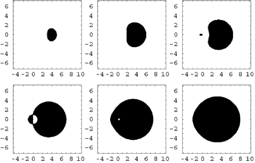
Figure 2: Lensed images of a top-hat circular source centered at $\zeta=(3,0)$ with a radius $L=1$ (top left), $L=2$ (top middle), $L=2.5$ (top right), $L=3$ (bottom left), $L=3.5$ (bottom middle), and $L=4$ (bottom right) in the source plane. An SIS lens is centered at $(0,0)$ in the lens plane. The Einstein radius is set to unity.

2.2 Gaussian source

In this subsection, we explore a circularly symmetric Gaussian source located at distance $\zeta_{0}$ from the center of an SIS lens. The surface brightness of a Gaussian circular source with standard deviation $L$ is

$$f(L,\zeta)=\frac{1}{2\pi L^{2}}\exp\biggl{[}-\frac{|\zeta|^{2}}{2L^{2}}\biggr{]}.$$ (8)

The magnification factor for a Gaussian circular source is then

$$\mu^{G}=\biggl{|}\int_{\textrm{all}}f(L,\zeta(z))dz\biggr{|}.$$ (9)

Figure 3: Magnification factor $\mu$ (solid curves) for a Gaussian circular source lensed by an SIS without background as a function of a standard deviation $L$ with distance from the lens center $\zeta_{0}=1$ (top curves), $\zeta_{0}=2$ (middle curves), and $\zeta_{0}=3$ (bottom curves) in comparison with those for an image with positive parity only (see eq. (10); dashed curves) and those for top-hat sources with a scaling $L\rightarrow\sqrt{8/\pi}L$ (here $L$ denotes a radius of a circular source) for the same $\zeta_{0}$ values (dotted curves).

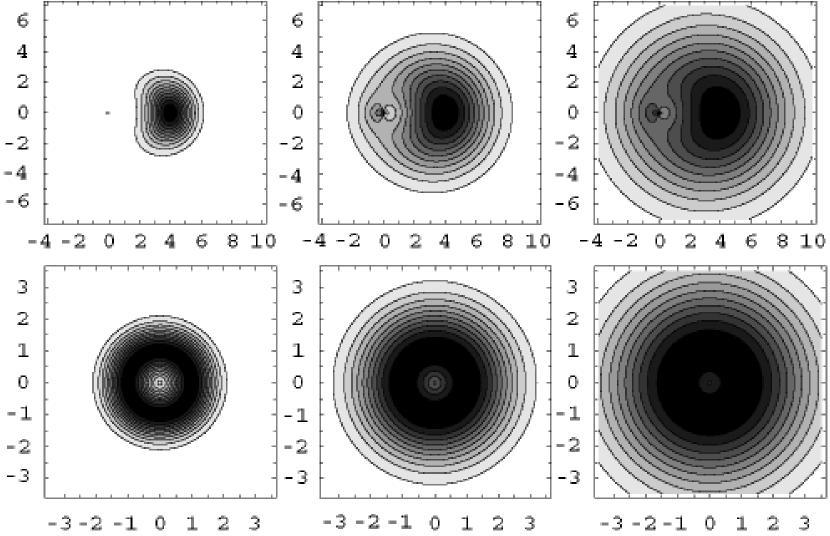
Figure 4: Top: Lensed images of a Gaussian circular source centered at $\zeta=(3,0)$ with a standard deviation $L=1$ (left), $L=2$ (middle), and $L=3$ (right). Bottom: Lensed images with the same parameters except for the position of the source at $\zeta=(0,0)$. An SIS lens is centered at $(0,0)$. Each interval between neighboring contours is 1/10 of the maximum value in the surface brightness. The Einstein radius is set to unity.

For an image with positive parity, equation (9) can be reduced to

$$\mu_{+}^{G}=-\frac{1}{2\pi L^{4}}\int_{0}^{\infty}dR\int_{0}^{2\pi}d\phi~{}\textrm{Re}~{}z_{+}\frac{\partial\textrm{Im}~{}z_{+}}{\partial\phi}R\exp\biggl{[}-\frac{R^{2}}{2L^{2}}\biggr{]}.$$ (10)

Expanding equation (10) in $\zeta_{0}$, we obtain the magnification factor $\mu$ in the large source size limit, $L\rightarrow\infty$, as

$$\mu^{G}\approx 1+(\pi/2)^{1/2}L^{-1}+L^{-2}/2.$$ (11)

As one can see in Figure 3, the contribution from an image with negative parity is negligible in the large source size limit. As in the top-hat model, the order of the leading term in $\mu-1$ is ${\cal{O}}(L^{-1})$. Therefore, the magnification effect for a Gaussian source cannot be negligible even if the source size is greater than the Einstein ring.

To estimate $\mu$ in the small source size limit $L\ll 1$, we introduce a cutoff radius $R_{\textrm{cut}}\sim L$ such that the contribution of integrand in equation (10) for $R>R_{\textrm{cut}}$ is negligible. If we further assume that $R_{\textrm{cut}}\ll 1<\zeta_{0}$, then equation (10) yields

$$\mu^{G}\sim\frac{R_{\textrm{cut}}^{4}}{2L^{4}}\biggl{(}1+\frac{1}{\zeta_{0}}\biggr{)}.$$ (12)

In the limit $\zeta_{0}\rightarrow\infty$, no magnification is expected, i.e., $\mu=1$. Therefore, we obtain the same formula for the small source size limit, $\mu^{G}\sim 1+\zeta_{0}^{-1}$ for $L\ll 1$ and $\zeta_{0}>1$, as in the top-hat model.

As one can see in Figure 3, for $L\gg\zeta_{0}+1$ the behavior of the magnification factor for a Gaussian source $\mu^{G}$ as a function of $L$ is similar to that of $\mu$ for a top-hat source, if an appropriate scaling for the source radius is carried out. Therefore, for an SIS, we conclude that the surface brightness profile does not play an important role in magnification in the large source size limit, provided that the source has a circular symmetry.

However, in the Gaussian model, distorted images have two distinct features depending on the position of the SIS : (1) a pair of bright and dark spots (dipole structure) at the position of the SIS where the spatial gradient in the surface brightness $\nabla f$ does not vanish (Figure 4, top), and (2) a dark spot (monopole structure) at the position of the SIS at the peak in the surface brightness where $\nabla f=0$ (Figure 4, bottom). As we see in section 4 and 5, these structures are not specific to SIS models. By looking into these small-scale “fine structures”, one can measure the density profile and the mass of the lens perturber.

3 SIS lens $+$ background shear and convergence

In this section, we show that in the large source size limit, the order of the (de)magnification perturbation of a circular top-hat source with radius $L$ (in units of an Einstein radius) owing to an SIS subhalo is typically ${\cal{O}}(L^{-1})$ with respect to that for an unperturbed lens. We model lensing by a subhalo locally as a background constant shear and convergence (Finch et al. 2002; Keeton 2003). If the mass scale of a substructure is sufficiently smaller than that of the macrolens, this model provides a good approximation in representing the local property of lensing along the line of sight to a substructure. For simplicity, we study a circular top-hat source centered at the SIS lens center.

3.1 Systematic distortion

First, we study the systematic distortion of a circular source. Let us consider an SIS lens with a one-dimensional velocity dispersion $\sigma$ and an external convergence $\kappa$ and shear $\gamma>0$. In the coordinates aligned to the shear, the lens equation is

$$\boldsymbol{\theta}_{y}=({\bf 1}-{\bf\Gamma})\boldsymbol{\theta}_{x}-\theta_{E}\frac{\boldsymbol{\theta}_{x}}{|\boldsymbol{\theta}_{x}|},$$ (13)

where

$${\bf\Gamma}=\left[\begin{array}[]{cc}\kappa+\gamma&0\\ 0&\kappa-\gamma\\ \end{array}\right]$$ (14)

and

$$\theta_{E}=4\pi\frac{\sigma^{2}}{c^{2}}\frac{D_{LS}}{D_{S}},$$ (15)

where $D_{S}$ is the angular diameter distance to the SIS lens, $D_{LS}$ is the distance between the SIS and the source, and $c$ is the light velocity. In terms of normalized coordinates, ${\bf x}=\boldsymbol{\theta}_{x}/\theta_{E}$ and ${\bf y}=\boldsymbol{\theta}_{y}/\theta_{E}$, the lens equation can be reduced to

$${\bf y}=({\bf 1}-{\bf\Gamma}){\bf x}-\frac{{\bf x}}{|{\bf x}|}.$$ (16)

To characterize the effect of background shear and convergence, we examine how a set of orthogonal vectors $(y_{1},0),(0,y_{2})$ in the source plane is mapped to another set of orthogonal vectors $(x_{1},0),(0,x_{2})$ in the lens plane that is aligned to the shear (i.e., astrometric shifts). From the lens equation (16), we have

$$x_{1} = \biggl{(}y_{1}+\frac{x_{1}}{|x_{1}|}\biggr{)}(1-\kappa-\gamma)^{-1}$$

$$x_{2} = \biggl{(}y_{2}+\frac{x_{2}}{|x_{2}|}\biggr{)}(1-\kappa+\gamma)^{-1}.$$ (17)

On the one hand, because of equation (17), the presence of an SIS perturber leads to a shift of a horizontal vector of the unperturbed image $(x_{1}>1,0)$ to $(x_{1}+1/(1-\kappa-\gamma),0)$, and a shift of a vertical vector of the unperturbed image $(0,x_{2}>1)$ to $(0,x_{2}+1/(1-\kappa+\gamma))$. On the other hand, as we have seen in section 2, for $\kappa=\gamma=0$, a circular top-hat source is isotropically magnified to a circular top-hat image with radius $1+L$. From these properties, we can expect that the boundary of the perturbed macrolensed image takes the form of an elliptic with a semi-major axis $a+1/(1-\kappa-\gamma)$ and a semi-minor axis $b+1/(1-\kappa-\gamma)$. The validity of this approximation is discussed in section 3.2.

Based on this approximation, distortion patterns are classified into three regimes by the sign of the eigenvalues of ${\bf 1}-{\bf\Gamma}$, $\xi_{1}\equiv 1-(\kappa+\gamma)$ and $\xi_{2}\equiv 1-(\kappa-\gamma)$:$(1)$ $\xi_{1}>0,\xi_{2}>0$ positive parity; (2) $\xi_{1}<0,\xi_{2}>0$ negative parity; and (3) $\xi_{1}<0,\xi_{2}<0$ doubly negative parity. As shown in Figure 5, in the positive parity case, both the semi-major axis and the semi-minor axis of an image extend by $\Delta a=\xi_{1}^{-1}$ and $\Delta b=\xi_{2}^{-1}$ in comparison with the unperturbed lensed image (background shear and convergence only) while in the doubly negative parity case, both axes shrink, i.e., $\Delta a<0$ and $\Delta b<0$. In the negative parity case, the semi-major axis shrinks by $|\Delta a<0|=|\xi_{1}^{-1}|$ whereas the semi-minor axis extends by $\Delta b=\xi_{2}^{-1}$ (Figure 6). Note, however, that a deviation from an elliptic is no longer negligible in the negative parity case, which is discussed in section 3.2.

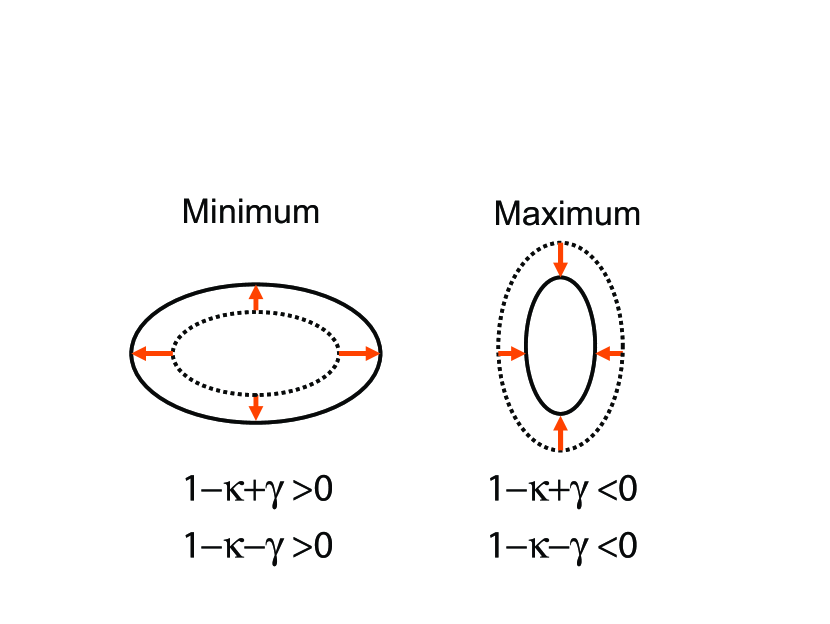
Figure 5: Systematic distortion by an SIS perturber at the center of a top-hat circular source with radius $L\gg 1$ in an external shear $\gamma$ and convergence $\kappa$. The dotted and solid closed curves show the boundaries of an unperturbed and a perturbed macrolensed image, respectively.

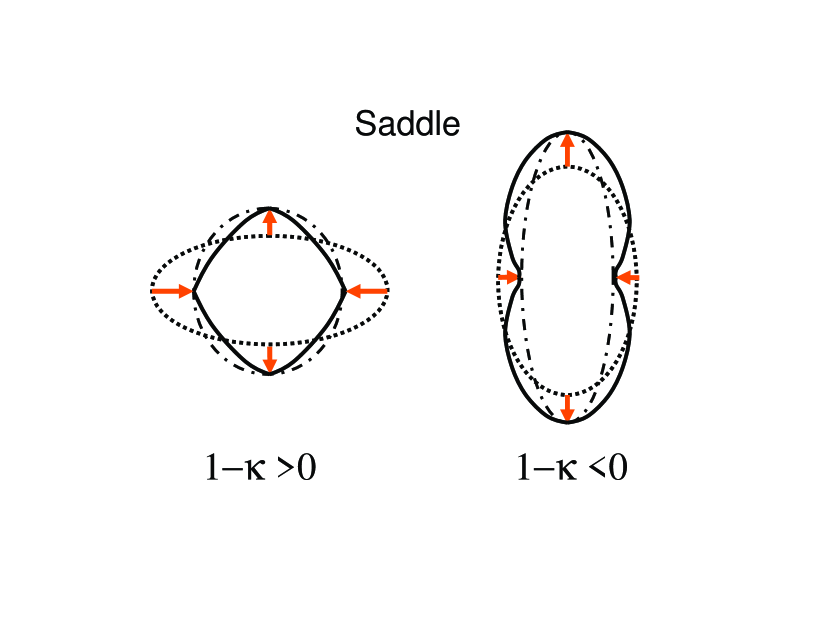
Figure 6: Systematic distortion by an SIS perturber at the center of a top-hat circular source in an external shear $\gamma$ and convergence $\kappa$. The dotted and solid closed curves show the boundaries of an unperturbed and a perturbed macrolensed image, respectively. The dash dotted closed curves are boundaries of an ellipse with a semi-major axis $a=(L-1)\xi_{1}^{-1}$ and a semi-minor axis $b=(L+1)\xi_{2}^{-1}$. The total area inside the boundary gets smaller (larger) than the unperturbed macrolensed image for $1-\kappa>0$ (for $1-\kappa<0$) provided that $L\gg 1$.

3.2 Systematic (de)magnification

In this subsection, we examine systematic (de)magnification for a lens that consists of an SIS plus a constant shear and a convergence that depends on the sign of the eigenvalues of ${\bf 1}-{\bf\Gamma}$. For simplicity, first, we consider a circularly symmetric top-hat source with radius $L\gg 1$ centered at the position of an SIS. Next, we compare our analytically calculated (de)magnification values with numerically calculated ones in cases where the source is placed at an off-center position.

First, we study the magnification effects in the positive parity case and the doubly negative parity case. As shown in Appendices B and C, in these cases, the shape of a distorted image perturbed by an SIS is well approximated by an ellipse, provided that $L\gg 1$ and $|1-\kappa|-\gamma\gg 0$. Therefore, a (de)magnification ratio defined as the ratio of the magnification for a perturbed lens (perturber + macrolens) to the magnification for an unperturbed caustics lens (macrolens only) $\chi(L)=\mu/\mu_{\textbf{bg}}$ can be simply written as

$$\chi(L)\approx 1+\frac{2\textrm{sgn}(\xi_{1})}{L}+\frac{1}{L^{2}}.$$ (18)

Thus, the order of the leading term in the (de)magnification perturbation defined as $\chi-1$ is $\sim{\cal{O}}(L^{-1})$. A perturbed image is always magnified (demagnified) in comparison with the unperturbed image in the positive (doubly negative) parity case. As shown in Figure 7 (left), the analytic formula (18) for a circular source centered at an SIS is accurate to within a few percent for $L\gg 1$. Even if a circular source is not centered at the SIS perturber, formula (18) still gives good accuracy for $L\gg 1$ as shown in Figure 8.

Next we consider the negative parity case. If the shape of an image perturbed by an SIS is well approximated by an ellipse, the (de)magnification ratio should be $\chi(L)=1-1/L^{2}$. However, in the negative parity case, distortion from an elliptic shape is no longer negligible at ${\cal{O}}(L^{-1})$. To quantify departure from an ellipse, we introduce two parameters $\epsilon(\theta)$ and $\eta(\theta)$ in the lens equation in polar coordinates that satisfy

$$L\cos(\theta+\eta) = a(1+\epsilon)(1-\kappa-\gamma)\cos\theta-a\cos\theta/R[a,b,\theta]$$

$$L\sin(\theta+\eta) = b(1+\epsilon)(1-\kappa+\gamma)\sin\theta-b\sin\theta/R[a,b,\theta],$$ (19)

where

$$a=(L+\textrm{sgn}(\xi_{1}))\xi_{1}^{-1},b=(L+\textrm{sgn}(\xi_{2}))\xi_{2}^{-1},$$ (20)

and

$$R[a,b,\theta]=(a^{2}\cos^{2}\theta+b^{2}\sin^{2}\theta)^{1/2}.$$ (21)

In terms of $\epsilon$, the ratio of the perturbed magnification factor to the unperturbed magnification factor can be approximately written as (see Appendix B)

$$\chi\approx\frac{4}{\pi}\int_{0}^{\pi/2}d\theta\bigl{(}(1+\epsilon)\cos\theta+\epsilon^{\prime}\sin\theta\bigr{)}(1+\epsilon)\cos\theta,$$ (22)

where $\epsilon^{\prime}=d\epsilon/d\theta$. As shown in Appendix B, the order of $\epsilon$ is ${\cal{O}}(L^{-1})$. Thus the order of the (de)magnification perturbation $\chi(L)-1$ is again ${\cal{O}}(L^{-1})$ in the large source size limit $L\gg 1$. Note that the analytic formula (22) can be used for any type of parity.

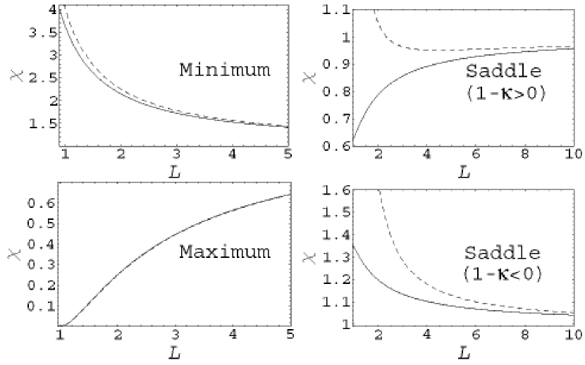
Figure 7: Comparison between numerically calculated magnification ratios $\chi$ (solid curves) and analytically calculated ones (dashed curves). For the maximum (positive parity) and minimum (doubly negative parity), eq. (18) is used, and for saddles (negative parity), eqs. (B1) and (22) are used. Parameters are $(\kappa,\gamma)=$(0.3,0.3) (top left), (2.5,0.2) (bottom left), (0.6,0.6) (top right), and (1.8,2.0) (bottom right). The center of an image is placed at ${\bf y}=$(0,0) in the source plane. The Einstein radius of an SIS lens is set to unity.

As shown in Figure 7, for $L\gtrsim 10$, the analytic formulae (18) and (22) for a source centered at an SIS give an accuracy to within a few percent with respect to the numerically calculated values. Because we expanded $\chi$ in $L^{-1}$, the expected error at the order ${\cal{O}}(L^{-1})$ is $\Delta\chi\sim{\cal{O}}(L^{-2})/(1+{\cal{O}}(L^{-1}))\sim(L(L+1))^{-1}$. For instance, we expect an error $\Delta\chi\sim 0.2$ for $L=2$ but $\Delta\chi\sim 0.01$ for $L=10$. If the distance between the boundaries of the source and caustics is very small, the magnification ratio $\chi$ is sensitive to the position of the lens. However, in the large source size limit $L\gg 1$, $\chi$ asymptotically converges to values given by formulae (18) and (22). In this case, as shown in Figure 8, (de)magnification is less sensitive to the position of the source provided that the caustics are totally occulted by the source. Our analytic formulae are very useful in representing the effects of background parameters $\kappa$ and $\gamma$ on systematic (de)magnification in such a case.

As we have seen, for typical values of convergence $\kappa$ and shear $\gamma$, the (de)magnification perturbation $1-\chi(L)$ can be as large as $1-\chi(L)\sim 0.4$ at $L\sim 5$ in the positive or doubly negative parity case. In other words, even if the source size is larger than the Einstein ring or caustics of an SIS perturber, the (de)magnification effects owing to the perturber are still prominent. In the negative parity case, the (de)magnification perturbation is smaller than for other parities $1-\chi(L)\sim 0.1$ at $L\sim 5$ for typical values of $\kappa$ and $\gamma$ but it still cannot be negligible at the order ${\cal{O}}(L^{-1})$.

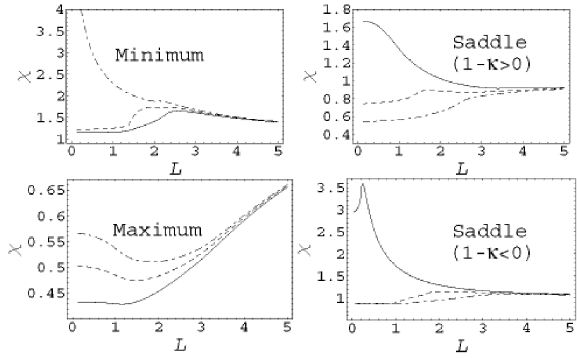
Figure 8: Magnification ratios $\chi$ as a function of radius $L$ of a circular top-hat source for $(\kappa,\gamma)=$(0.3,0.3) (top left), (2.5,0.2) (bottom left), (0.7,0.7) (top right), and (1.8,2.0) (bottom right) for different image positions centered at ${\bf y}=$(2,0) (solid curves), (1,1) (dashed curves), (0,2) (dash dotted curves) in the source plane. The Einstein radius of an SIS lens is set to unity. An increase at $L\lesssim 2$ in the minimum and saddle cases is owing to a crossing with a caustic.

3.3 Mean (de)magnification for a point source

Our results for the systematic (de)magnification effects for a circular top-hat source centered at the lens center can be applied to the study of the mean (de)magnification for a point source within a radius $L$ from the lens center.

For a point source at ${\bf y}={\bf y}_{s}$ in the source plane in which a lens perturber is put at the center, the magnification factor corresponding to an image ${\bf x}={\bf x}({\bf y}_{s})$ is written as

$$\mu=\biggl{|}\frac{\partial{\bf x}}{\partial{\bf y}}\biggr{|}_{{\bf y}={\bf y}_{s}}.$$ (23)

Then the magnification factor averaged over a disk with radius $L$ centered at the center in the source plane is

$$\langle\mu\rangle_{L}\equiv\frac{1}{4\pi L^{2}}\int_{|{\bf y}|\leq L}d{\bf x}.$$ (24)

This is equivalent to the magnification factor for a top-hat circular source with radius $L$ centered at the lens center.

The obtained mean magnification factor $\langle\mu\rangle_{L}$ is related to the lensing cross section $\sigma(\delta)$ which is defined as the cross section for a magnification perturbation stronger than $\delta$ (Keeton 2003). Conversely, we can define the mean magnification perturbation for a cross section $\sigma=4\pi L^{2}$ centered at the perturber as $\langle\delta\rangle_{L}\equiv 1-\langle\mu\rangle_{L}/\mu_{\textbf{bg}}$. The mean magnification is useful for lensing systems in which the macro-lensing parameters are precisely determined. Comparing an observed value of the perturbation $\delta$ with a computed mean perturbation and its variance, one can constrain the size of the cross section in units of the area of an Einstein disk of a perturber, provided that the source size is negligible in comparison with the Einstein ring.

Thus, our results are useful not only for estimating the magnification for extended sources larger than the Einstein ring but also for estimating the mean magnification perturbation for a point source in substructure lensing (see also Metcalf & Madau 2001; Chiba 2002; Dalal & Kochanek 2002).

4 Measurement of velocity dispersion and distance

In this section, we study how one can break the degeneracy between the lensing effects of the velocity dispersion (or total mass) of a lens perturber and those of its distance along the line of sight by measuring distortion in the extended images.

Suppose that a halo at redshift $z=z_{h}$ deflects light from a source at redshift $z_{s}$ by an angle $\hat{\boldsymbol{\alpha}}_{h}$ and a clump at redshift $z=z_{c}\leq z_{h}$ deflects the light by an angle $\hat{\boldsymbol{\alpha}}_{c}$ (see Figure 9). The normalized lens equations for an unperturbed system and a perturbed system are

$${\bf y}={\bf x}_{0}-\boldsymbol{\alpha}_{h}({\bf x}_{0}),$$ (25)

and

$${\bf y}={\bf x}_{0}-\boldsymbol{\alpha}_{c}({\bf x}-{\bf x}_{c})-\boldsymbol{\alpha}_{h}({\bf x}^{\prime}),$$ (26)

respectively (Schneider et al. 1992). Here, ${\bf y}$ is the position of a source, ${\bf x}$ is the position of an image in the microlens plane, ${\bf x}_{c}$ is the position of a clump, and ${\bf x}^{\prime}$ is the position of an intersection between the light ray and the macrolens plane. The normalized angle is defined as $\boldsymbol{\alpha}_{x}\equiv D(z_{x},z_{s})/D_{s}\theta_{E}$, where $D(z_{x},z_{s})$ is the angular diameter distance between an object at redshift $z_{x}$ and a source at redshift $z_{s}$, $D_{s}$ is the distance to the source, and $\theta_{E}$ is the Einstein radius of the macrolens.

From the lens equation for the microlens system, we have

$${\bf x}^{\prime}={\bf x}-\beta\boldsymbol{\alpha}_{c}({\bf x}-{\bf x}_{c}),$$ (27)

where the factor

$$\beta=\frac{D_{ch}D_{s}}{D_{cs}D_{h}}$$ (28)

encodes a distance ratio written in terms of the distance between the clump and halo $D_{ch}$, the distance between the clump and source $D_{cs}$, and the distance to the halo $D_{h}$.

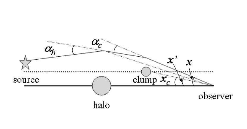
Figure 9: Light from a source deflected by a halo at $z_{h}$ and a clump at $z_{c}<z_{h}$.

In what follows, we assume that the Einstein radius of the clump is much smaller than that of the halo, i.e., $|{\bf x}^{\prime}-{\bf x}_{0}|\ll 1$. Then the deflection angle is approximately given by (Keeton 2003)

$$\boldsymbol{\alpha}_{h}({\bf x}^{\prime})\sim\boldsymbol{\alpha}_{h}({\bf x}_{0})+{\bf\Gamma}({\bf x}-\beta\boldsymbol{\alpha}_{c}({\bf x}-{\bf x}_{c})-{\bf x}_{0}),~{}~{}~{}{\bf\Gamma}=\frac{\partial\boldsymbol{\alpha}_{h}}{\partial{\bf x}}\biggr{|}_{{\bf x}_{0}},$$ (29)

where ${\bf\Gamma}$ represents the convergence and shear for the unperturbed macrolens. From equations (27), (28) and (29), we obtain an effective lens equation for a perturbed system,

$$\tilde{{\bf y}}=({\bf 1}-{\bf\Gamma}_{\textrm{eff}})\tilde{{\bf x}}-\boldsymbol{\alpha}_{c}(\tilde{{\bf x}}),$$ (30)

where

$$\tilde{{\bf x}}\equiv{\bf x}-{\bf x}_{c},\tilde{{\bf y}}\equiv-({\bf 1}-{\bf\Gamma})({\bf 1}-\beta{\bf\Gamma})^{-1}({\bf x}_{c}-{\bf x}_{0}),$$ (31)

and

$${\bf\Gamma}_{\textrm{eff}}={\bf 1}-({\bf 1}-{\bf\Gamma})({\bf 1}-\beta{\bf\Gamma})^{-1}.$$ (32)

Here $\tilde{{\bf y}}$ is the effective source position that satisfies $\tilde{{\bf y}}=(1-\beta{\bf\Gamma})^{-1}{\bf y}$ if the convergence $\kappa$ and the shear $\gamma$ are constant. As a function of the convergence $\kappa$ and shear $\gamma$ in the unperturbed macrolens and the distance ratio $\beta$, the effective convergence and shear can be expressed as

$$\kappa_{\textrm{eff}}=\frac{(1-\beta)(\kappa-\beta(\kappa^{2}-\gamma^{2}))}{(1-\beta\kappa)^{2}-\beta^{2}\gamma^{2}},\gamma_{\textrm{eff}}=\frac{(1-\beta)\gamma}{(1-\beta\kappa)^{2}-\beta^{2}\gamma^{2}}.$$ (33)

In what follows, we assume that ${\bf\Gamma}$ is a constant matrix that does not depend on the image position ${\bf x}$ , i.e., $\boldsymbol{\alpha}_{h}={\bf\Gamma}$, and we also assume that an SIS perturber is placed at the center of the image plane ${\bf x}_{c}=(0,0)$ , i.e. $\boldsymbol{\alpha}_{c}({\bf x})=\theta_{Ep}~{}{\bf x}/|{\bf x}|$, where $\theta_{Ep}$ is the Einstein radius of the SIS perturber.

Now consider an astrometric shift of an image $\Delta{\bf x}={\bf x}-{\bf x}_{0}$ that is defined as the difference between a perturbed macrolensed image position ${\bf x}$ and an unperturbed macrolensed image position ${\bf x}_{0}$ that satisfies ${\bf y}=({\bf 1}-{\bf\Gamma}){\bf x}_{0}$. From equation (31), one can see that an effective image position $\tilde{{\bf x}}_{0}$ that satisfies $\tilde{{\bf y}}=({\bf 1}-{\bf\Gamma}_{\textrm{eff}})\tilde{{\bf x}}_{0}$ is equal to the unperturbed macrolensed image position ${\bf x}_{0}$. Then the astrometric shift of an image with respect to the unperturbed image can be written as $\Delta{\bf x}={\bf x}-\tilde{{\bf x}}_{0}$. Taking coordinates ${\bf x}=(x_{1},x_{2})$ aligned to the shear, astrometric shifts of images on the horizontal axis $x_{1}$ are $\Delta{\bf x}_{\parallel}=\theta_{Ep}/(1-\kappa_{\textrm{eff}}-\gamma_{\textrm{eff}})$ and those of images on the vertical axis $x_{2}$ are $\Delta{\bf x}_{\perp}=\theta_{Ep}/(1-\kappa_{\textrm{eff}}+\gamma_{\textrm{eff}})$. Plugging the relations in equation (33) into these shifts, one can see that the distance ratio $\beta$, and the Einstein radius $\theta_{Ep}$ of the perturber can be determined from observed values of astrometric shifts $\Delta{\bf x}_{\parallel}$ and $\Delta{\bf x}{\perp}$ provided that parameters $\kappa$ and $\gamma$ are determined from the best-fit macrolens model. Furthermore, if the macrolens parameters such as $D_{s}$, $D_{h}$, and $D_{hs}$ are known, then one can measure the distance between the SIS perturber and the macrolens from the distance ratio $\beta$ and the velocity dispersion of the SIS.

The accuracy in the measured distance ratio $\beta$ for a given resolution can be estimated from an astrometric shift $\Delta{\bf x}={\bf x}-{\bf x}_{0}$ of a perturbed image with respect to the unperturbed image. As we have seen, in the coordinates aligned to the background shear, the $\beta$ dependence of the horizontal shift for unperturbed images on the horizontal axis ${\bf x}_{1}$ is $\Delta x_{1}=\theta_{Ep}(1-\beta(\kappa+\gamma))/(1-\kappa-\gamma)$. As $\beta$ increases from $0$ to $1$, $\Delta x_{1}$ decreases by $\Delta(\Delta x_{1})=\theta_{Ep}(\kappa+\gamma)/(1-\kappa-\gamma)$. Therefore, for macrolenses with $(\kappa+\gamma)/(1-\kappa-\gamma)={\cal{O}}(1)$, the necessary angular resolution is $\Delta\theta\sim\theta_{Ep}$ in order to determine $\beta$ with a relative accuracy $\Delta\beta/\beta<1$. In other words, $\beta$ can be measured from a horizontal shift $\Delta x_{1}$ with good accuracy if the angular resolution is comparable to the Einstein radius of the SIS perturber. Similarly, the $\beta$ dependence of the vertical shift for unperturbed images on the vertical axis $x_{2}$ is $\Delta x_{2}=\theta_{Ep}(1-\beta(\kappa-\gamma))/(1-\kappa+\gamma)$. Therefore, for macrolenses with $\kappa\sim\gamma$, the $\beta$ dependence of vertical shifts $\Delta x_{2}$ can be observed with an angular resolution $\Delta\theta\sim(\kappa-\gamma)\theta_{Ep}$. In other words, one needs to resolve an image that is significantly smaller than the Einstein radius of an SIS perturber if $\kappa\sim\gamma$. However, as we have seen in section 2, the Einstein radius $\theta_{Ep}$ can be directly measured by the size of the dipole structure where the surface brightness gradient at the position of the SIS perturber is non vanishing (see also section 5). Therefore, we conclude that $\beta$ can be measured from the observed horizontal astrometric shift $\Delta{\bf x}_{\parallel}$ with respect to an unperturbed image if observation with an angular resolution $\Delta\theta\sim\theta_{Ep}$ is achieved.

In practice, however, we should pay attention to various factors that complicate the lens system. First, the observed distortion can be caused by distortion of the source itself. However, this is not a serious problem for multiply imaged lensing systems. By comparing a lensed image with other images, we can easily distinguish whether the distortion pattern is associated with the source properties or not. Second, the SIS perturber might not be spherically symmetric. Third, our assumption of an SIS density profile for perturbers may not be correct. Fourth, perturbers may not be single. Finally, the center of the perturber may not lie on the center of the source. The second and the third problems can be solved by measuring the distortion inside the Einstein radius of the perturber, which is discussed in section 5. To solve the fourth and the last problems, we need a source with spatially varying surface brightness. Substructures in a QSO jet are good examples. If the position of the perturber is known, we can draw a set of coordinates for which the perturber resides at the center. Then we can assign position vectors to each substructure in the extended source, which will restrict the lens parameters that can characterize the microlens such as $\beta$ and $\theta_{Ep}$. In other words, a sufficient number of substructures of an image can restrict the substructure lensing parameters.

5 Measurement of mass density profile

From a reconstruction of a mapping between a macrolensed source image and a microlensed image, we can extract information of the mass density profile of the perturbers. To do so, we need to resolve distorted images within the Einstein radius of a perturber. Let us first consider a simple lens model that consists of a source $S$ with a circular symmetry whose surface brightness obeys a Gaussian distribution with a standard deviation $\sigma$,

$$f_{g}(y,\sigma)=\frac{1}{\sqrt{2\pi}\sigma}\exp{\biggl{[}-\frac{y^{2}}{2\sigma^{2}}\biggr{]}},$$ (34)

and a lens (i.e. a perturber) $P$ with a circular symmetry. For simplicity, we consider a polynomially suppressed mass density profile for the lens $P$.

First, we consider a system in which a lens is put in the direction of the line of sight to the center of the source. Then we have the lens equation

$${\bf y}={\bf x}-\frac{{\bf x}}{|{\bf x}|^{\alpha}},$$ (35)

where $\alpha$ corresponds to the power of the polynomially suppressed mass density profile of $P$. For instance, $\alpha=2$ corresponds to a point mass, and $\alpha=1$ corresponds to an SIS. From equation (34) and (35), for $\alpha>0$, we obtain the surface brightness profile $f(x)$ in the neighborhood of a lens $x=|x|\ll 1$ as,

$$\ln f(x)\approx-\frac{x^{2}}{2\sigma^{2}|x|^{2\alpha}}-\ln{\sqrt{2\pi}\sigma}.$$ (36)

In Figure 10, one can clearly see the difference in the surface brightness of lensed images that depends on the mass density profile of the lens. For a lens with $1<\alpha$, the surface brightness vanishes toward the center of a lens as $\ln f(x)\sim-x^{2-2\alpha}$. This is because the outer dimmed region of the source is mapped into the neighborhood of the center of the lens. Consequently, one would observe a “black hole” at the position of a point mass lens if $\alpha=2$. In contrast, the surface brightness is finite in the neighborhood of the center of an SIS lens. In this case, a region ${R:|y|<1}$ is mapped into a region ${R^{\prime}:|x|<1}$ on the opposite side (with opposite sign) within the Einstein radius but any regions outside the Einstein radius are not mapped into a region inside the Einstein radius. Hence, one would see a “dark hole” instead of a “black hole” for an SIS lens. If the mass density profile of a lens is shallower than that of an SIS lens, i.e. $\alpha<1$, then one would see a bright spot surrounded by a dark hole, because the mass concentration is so weak that the bending angle for a light ray that departed from the brightest region of the source is very small.

In real observations, the detectability of these features strongly depends on the resolution of the map and the linear scale $\sigma$ in which the surface brightness varies. As $\sigma$ gets larger, variability in the surface brightness of the lensed image within an Einstein radius gets smaller as $\propto\sigma^{-1}$ (see Figures 10 and 11). To determine $\sigma$ or equivalently, the Einstein radius of a perturber and $\alpha$, one needs to measure a mapping between the source plane and the lens plane. Suppose that we observe a “dark hole” at a peak in the surface brightness of the source. If there are peaks or dips at $y_{i}>1$ in the source, then mapped images of these structures should be observed inside dark holes at $x_{i}<1$. From more than two sample points of these structures, one can determine the model parameters $\sigma$ and $\alpha$. Even if circular symmetry in the projected mass distribution of the perturber is broken, a sufficient number of sample points can determine the lens parameters such as ellipticity and external shear that describe distortion from a circular symmetry. For instance, in a QSO-galaxy lens system, observation of astrometric shifts of subjects in a QSO jet with respect to a macrolensed image may determine the model parameters for perturber lenses.

Next we consider lens systems in which the lens is not placed at the peak of the source. As shown in Figure 11, we would observe a pair of dark and bright spots at the position of the lens where the radial derivative in the surface brightness does not vanish. For $1\leq\alpha<2$, the surface brightness vanishes at the position of the lens because the outer dimmed region is mapped inside the Einstein radius. For $\alpha=1$, the surface brightness is finite at the position of the lens but the radial derivative of the surface brightness at the position of the lens diverges even if the surface brightness of the source is smooth. As in the former case, from more than two sample points, one can determine the model parameters $\sigma$ and $\alpha$.

Our assumption of a Gaussian form of the surface brightness of a source may be too idealized. In order to estimate the effects of deviation from the Gaussian distribution, we consider small-scale fluctuations in the background source. For simplicity, we added Gaussian fluctuations with a standard deviation that is 1/15 of the background Gaussian peak value and with a vanishing mean to the smooth background Gaussian source. We calculated lensed images for two examples with the same smoothed source parameters as in the previous cases, namely, $\sigma=2$ and $y=-1$ (large surface brightness gradient), and $\sigma=10$ and $y=-5$ (small surface brightness gradient). The minimum wavelength of the Fourier mode of an additional fluctuation is assumed to be $\lambda_{\textbf{min}}=1/4$. As shown in Figure 12, a discontinuous change in the surface brightness for a point mass is still apparent for both cases, whereas for an SIS, such a discontinuous change is less apparent for the case with a small-scale brightness gradient (right). This is because for an SIS, an observable astrometric shift is limited to images within the Einstein ring of the perturber. Therefore, in order to measure the density profile of an SIS, we need a source whose (smoothed) surface brightness gradient is sufficiently large.

Figure 10: Left: Surface brightness of lensed images for $\alpha=2$ (thin solid curve), 1.5 (dashed curve), 1 (dotted curve), and 0.8 (dash dotted curve) for a circularly symmetric Gaussian source with $\sigma=1$ (thick solid curve). The horizontal axis denotes a coordinate $x$ in the image plane. The Einstein radius of a perturber is set to unity. A lens is put at the peak of the Gaussian distribution. Right: Same parameters as in the left panel, expect for the standard deviation $\sigma=4$.

Figure 11: Same parameters as in Figure 10 expect for the standard deviation $\sigma$ and the position of the lens. Left: $\sigma=2$ and a source is put at $y=-1$ in the source plane. Right: $\sigma=10$ and a source is put at $y=-5$ in the source plane.

Figure 12: Effects of small-scale fluctuations in the surface brightness of the source. The parameters are the same as in Fig. 11, except for additional Gaussian fluctuations with a standard deviation equal to 1/15 of the Gaussian peak of the smooth background and a mean equal to 0. The minimum wavelength of the fluctuation is assumed to be $\lambda_{\textbf{min}}=1/4$. Thick solid curves denote the surface brightness $f$ of the source, and thin solid curves and dotted curves correspond to the surface brightness of an image for $\alpha=2$ (point mass) and $\alpha=1$ (SIS), respectively.

6 Summary

In this paper, we have explored the extended source size effects in substructure lensing. First, we have shown that for a simple SIS lens model with a circular top-hat or Gaussian surface brightness profile, the magnification effect is prominent even if the source size is larger than the size of an Einstein ring. Second, we have analyzed SIS lens systems with background shear $\gamma$ and convergence $\kappa$ relevant to substructure lensing. We have derived analytic (de)magnification asymptotic formulae in the large source size limit for three types of parity of an image, namely, positive, negative, and doubly negative parities. In the positive (doubly negative) parity case, the source is always magnified (demagnified) in comparison with the unperturbed macrolens. In the negative parity case, magnification depends on the sign of $1-\kappa$. For $1-\kappa>0$, the source tends to be slightly magnified, whereas it tends to be slightly demagnified for $1-\kappa<0$. Again, we find that in the large source size limit, the order of the (de)magnification perturbation $1-\chi(L)$ with respect to the unperturbed one is typically ${\cal{O}}(L^{-1})$, where $L$ is the source radius in units of an Einstein radius. We have also shown that these results are relevant to the mean (de)magnification for a point source at a distance $L$ from the lens perturber center. Third, we have shown that one can break the degeneracy between the lensing effects of mass and distance of a substructure based on the distortion pattern in the perturbed image provided that the lensing parameters of macrolensing are determined from the position and flux of multiple images. Finally, we have shown that the density profile of a substructure is directly measured by reconstructing the mapping between a perturbed lens system (macrolensing + microlensing) and an unperturbed one (macrolensing only), which can be achieved by resolving an image within the Einstein radius of a substructure.

Although it seems that our results may not be relevant to current observations of substructure lenses, they will surely become important tools in future observations with improved sensitivity and angular resolution. For instance, if the sensitivity in the measured flux is dramatically improved, then we may be able to find an asymptotic regime in which the magnification perturbation is inversely proportional to the size of the source with a common center of light. Future observations of QSO jets in the radio band or of cold dusts in starburst galaxies in submillimeter band may reveal such systems if observed with different frequencies. If the proper source size is known, then we can determine the angular size of the Einstein radius of a lens perturber. Similarly, if the angular resolution were dramatically improved, then we would be able to get a fruitful amount of information from a substructure within a source. For instance, a QSO jet usually consists of two jet components plus a center nucleus. Each jet sometimes has some small subjects or small-scale structures. Then we could determine the spatial variation within the source in the global linear maps between macro lensed images by comparing their substructures. Mapping cold dusts around a QSO in a QSO-galaxy lens at the submillimeter band with an angular resolution of $\sim 10$ mas may directly determine the distance to a $\sim 10^{8}-10^{9}M_{\odot}$ subhalo near the center of the lens galaxy (Inoue & Chiba 2005). Breaking the mass-distance degeneracy and a precise measurement of mass density profile of a perturber might both be achieved by such an observation.

In reality, lensing systems are usually much more complex and modeled with a large number of parameters (often too many!). For instance, a macrolens can be perturbed by a number of subhalos with different projected masses, ellipticities, and distances from the source. The corresponding best-fit parameters can be determined by minimizing a certain measure between an observed image and a reconstructed image based on a certain lensing model.

Many important issues that we have omitted are (1) irregularity in the source shape, (2) irregularity in the mass density profile of each perturber, (3) time varying source effects, (4) the effect of multiple perturbers, and (5) lensing parameter error estimates. In real observations, we always have to tackle all these problems. We will soon address these issues in our future work.

Appendix A Analytical treatment of overlapping region

We consider a circularly symmetric top-hat source disk $D$ with a radius $L$ located at a distance $\zeta_{0}$ from the center of an SIS lens. The magnification factors for an image with positive parity and negative parity can be written in terms of the radius $L$ and $\zeta_{0}$ as in equation (5).

For $\zeta_{0}-L>1$, there is no overlapping region between a source disk $D$ and a unit Einstein ring $E$, so the total magnification is $\mu\equiv\mu_{+}+\mu_{-}=\mu_{+}$. For $\zeta_{0}-L<-1$, an Einstein ring $E$ is totally included in a source disk $D$, and so we have $\mu=\mu_{+}+\pi\mu_{-}(L=1,\zeta_{0}=0)/\pi L^{2}=\mu_{+}+1/L^{2}$. For $\zeta_{0}<1$, if a source disk $D$ is totally included in an Einstein ring $E$, i.e., $L<|1-\zeta_{0}|$, then $\mu=\mu_{+}+\mu_{-}$. These results are summarized in table 1.

Table 1: Three Different Cases for Magnification of a Circular Top-hat Source

Case	no overlapping	$D\subset E$	$E\subset D$
$\mu$	$\mu_{+}$	$\mu_{+}+\mu_{-}$	$\mu_{+}+1/L^{2}$

For other cases in which there are some overlaps between a source disk $D$ and an Einstein ring $E$, namely, $|\zeta_{0}-1|<L<\zeta_{0}+1$, it is difficult to obtain a simple explicit formula. However, for the cases $L>1$ and $\zeta_{0}\gg 1$ overlapping some part of an Einstein ring $E$, a simple approximated formula can be obtained as follows. In coordinates $(L,\mu(L))$, we may connect two points A, $(\zeta_{0}-1,\mu_{+}(\zeta_{0}-1))$, and B, $(\zeta_{0}+1,\mu_{+}(\zeta_{0}+1))$, simply by a segment, because the area of the overlapping region $E\cup D$ is a monotonically increasing function of $L$. However, the derivatives at A and B are not continuous. Instead, we can connect A and B by a smooth function whose derivatives vanish at A and B, because the derivatives $d\mu/dL$ at $L=\zeta_{0}-1$ and at $L=\zeta_{0}+1$ are very small for $\zeta_{0}\gg 1$. A simple choice of such a function is

$$\delta\mu(s,L,\zeta_{0})=\frac{\textrm{Erf}(s(L-\zeta_{0}))-\textrm{Erf}(-s(L-\zeta_{0}))+2}{4L^{2}},$$ (A1)

where $s>0$ controls smoothness of $\delta\mu$ around $L=\zeta_{0}$. Then we can approximate the magnification factor $\mu$ as

$$\mu(L,\zeta_{0})\approx\mu_{+}(L,\zeta_{0})+\delta\mu(s,L,\zeta_{0}),~{}~{}~{}L>1,\zeta_{0}>1.$$ (A2)

We find that $s\sim 3$ leads to an accuracy within a few percent for $\zeta_{0}>1$ (see Figure 1). Note that our approximated formula (A2) fails for $\zeta_{0}<1$ and $L<1+\zeta_{0}$ because the contribution from $\mu_{-}$ cannot be negligible in that case. If $\zeta_{0}\ll 1$, then $\mu$ can be approximated as

$$\mu(L,\zeta_{0})\approx\mu_{+}(L,0)+\mu_{-}(L,0)H(1-L),$$ (A3)

where $H$ is a Heaviside step function.

Appendix B Deformation parameters in the negative parity case

Assuming $\eta\ll 1$, equation (19) can be solved as

$$\epsilon(\theta) = (b(1-\kappa+\gamma))^{-1}\Biggl{\{}L-b\bigl{(}(1-\kappa+\gamma)-R^{-1}\bigr{)}-\Biggl{(}\cos^{2}\theta\bigl{(}b(1-\kappa+\gamma)LR$$ (B1)

$$+ a(2b\gamma-(1-\kappa-\gamma)LR)\bigr{)}\Biggr{)}/R\bigl{(}a(-1+\kappa+\gamma)\cos^{2}\theta+b(-1+\kappa-\gamma)\sin^{2}\theta\bigr{)}\Biggr{\}},$$

and

$$\eta(\theta)=\frac{\cos\theta\sin\theta\bigl{(}b\xi_{2}+a(2b\gamma/(LR)-\xi_{1})\bigr{)}}{a\xi_{1}\cos^{2}\theta+b\xi_{2}\sin^{2}\theta}.$$ (B2)

In the negative parity case, the approximated solution of $\epsilon\sim{\cal{O}}(L^{-1})$ for $L\gg 1$ is

$$\epsilon(\theta)\approx L^{-1}\biggl{[}-1+2\cos^{2}\theta+\frac{\sin^{2}\theta}{(1-\kappa+\gamma)F(\kappa,\gamma,\theta)}+\frac{\cos^{2}\theta}{(1-\kappa-\gamma)F(\kappa,\gamma,\theta)}\biggr{]},$$ (B3)

where

$$F(\kappa,\gamma,\theta)=\sqrt{\frac{\cos^{2}\theta}{(1-\kappa-\gamma)^{2}}+\frac{\sin^{2}\theta}{(1-\kappa+\gamma)^{2}}}.$$ (B4)

Now, we evaluate a mean value of $\epsilon$ averaged over $\theta$ in the negative parity case. For $1-\kappa>0$, we have $|1-\kappa+\gamma|^{-1}<|1-\kappa-\gamma|^{-1}$. Therefore, the contribution of the integrand $\cos^{2}\theta/(1-\kappa-\gamma)F$ is dominant over $\sin^{2}\theta/(1-\kappa+\gamma)F$. Note that the amplitudes of both integrands are 1. Because $\langle-1+2\cos^{2}\theta\rangle_{\theta}=0$, we have $\langle e\rangle_{\theta}<0$. Thus, the area of the perturbed image tends to become smaller than that of an elliptic disk $D$ with a semi-major axis $a$ and a semi-minor axis $b$ at ${\cal{O}}(L^{-1})$. For $1-\kappa<0$, we have $|1-\kappa+\gamma|^{-1}>|1-\kappa-\gamma|^{-1}$. Therefore, the contribution of the integrand $\sin^{2}\theta/(1-\kappa+\gamma)F$ is dominant over $\cos^{2}\theta/(1-\kappa-\gamma)F$, leading to $\langle e\rangle_{\theta}>0$. In this case, the area of the perturbed image tends to become larger than that of $E$ (see Figure 6). In summary, we expect a magnification ratio $\chi>1$ for $1-\kappa<0$ but demagnification, $\chi<1$ for $1-\kappa>0$.

As for $\eta$, equation (B2) yields

$$\eta(\theta)\approx L^{-1}\sin 2\theta\biggl{(}1+\frac{\gamma}{((1-\kappa)^{2}-\gamma^{2})F(\kappa,\gamma,\theta)}\biggr{)}.$$ (B5)

Because $\gamma/((1-\kappa)^{2}-\gamma^{2})F\lesssim 1$, we have $\eta\lesssim L^{-1}$. Thus, an assumption of $\eta\ll 1$ is correct for $L\gg 1$.

Appendix C Deformation parameters in the positive and doubly negative parity cases

To evaluate the accuracy of equation (18), we calculate the deformation parameters $\epsilon$ and $\eta$. In the positive parity case, the semi-major axis and semi-minor axis of an ellipse $\tilde{D}$ that represents an approximated shape of the perturbed lensed image are $a=(L+1)\xi_{1}^{-1}$ and $b=(L+1)\xi_{2}^{-1}$. Plugging these values into equation (B3), we obtain

$$\epsilon(\theta)\sim L^{-1}\Biggl{(}\frac{1-\kappa+\gamma\cos 2\theta}{((1-\kappa)^{2}-\gamma^{2})F(\kappa,\gamma,\theta)}-1\Biggr{)}.$$ (C1)

The order of $\epsilon$ is evaluated in terms of the median $(1-\kappa)/((1-\kappa)^{2}-\gamma^{2})>0$ of $F$ as

$$\epsilon(\theta)\sim L^{-1}\Biggl{(}\frac{\gamma\cos 2\theta}{1-\kappa}\Biggr{)}.$$ (C2)

Therefore, for $1-\kappa-\gamma\gg 0$, the effect of deformation from an ellipse $\tilde{D}$ is negligible at ${\cal{O}}(L^{-1})$.

In the doubly negative parity case, we have $a=(L-1)\xi_{1}^{-1}$ and $b=(L-1)\xi_{2}^{-1}$. In a similar manner, one can show that

$$\epsilon(\theta)\sim L^{-1}\Biggl{(}\frac{\gamma\cos 2\theta}{-1+\kappa}\Biggr{)}.$$ (C3)

Therefore, for $-1+\kappa-\gamma\gg 0$, the effect of deformation from an ellipse $\tilde{D}$ is again negligible at ${\cal{O}}(L^{-1})$.

References

- (1)
- (2) Agol, E., Jones, B., & Blaes, O. 2000, ApJ, 545, 657
- (3) Bradac, M., Schneider, P., Steinmetz, M., Lombardi, M., & King, L. J., 2002, A&A, 388, 373
- (4) Chiba, M. 2002, ApJ, 565, 17
- (5) Chiba, M., Minezaki, T., Kashikawa, N., Kataza, H., & Inoue, K. T. 2005, ApJ, 627, 53
- (6) Dalal, N.& Kochanek, C. S. 2002, ApJ, 572, 25
- (7) Dobler, G. & Keeton, C. R. 2005, astro-ph/0502436
- (8) Evans, N. W. & Witt, H. J. 2003, MNRAS, 345 1351
- (9) Finch, T., Carlivati, L. P., Winn, J. N. & Schechter, P. L. 2002, ApJ, 577, 51
- (10) Hirabayashi, H. et al. 2001, in ASP Conf. Ser. 251, New Century of X-ray Astronomy, eds. H. Inoue, & H. Kunieda, (San Francisco: ASP), 540
- (11) Inoue, K. T. & Chiba, M. 2003, ApJ, 591, L83
- (12) Inoue, K. T. & Chiba, M. 2005, ApJ, 633, 23
- (13) Kadler, M., Ros, E., Zensus, J.A., Lobanov, A.P. & Falcke H. 2003, in SIF Conf. Proc. 81, SRT: The Impact of Large Antennas on Radioastronomy and Space Science, eds. N. D’ Amico et al. (Bologna: Italian Phys. Soc.), 219
- (14) Kameno, S., Inoue, M. & Fujisawa K. 2000, PASJ, 52, 1045
- (15) Keeton, C. R., 2003, ApJ, 584, 664
- (16) Keeton, C. R., Gaudi, B.S., & Petters, A. O., 2003, ApJ, 598, 138
- (17) Klypin, A., Kravtsov, A. V., Valenzuela, O., & Prada, F. 1999, ApJ, 522, 82
- (18) Mao, S. & Schneider, P. 1998, MNRAS, 295, 587
- (19) Metcalf, R. B. & Madau, P. 2001, ApJ, 563, 9
- (20) Metcalf, R. B. & Zhao, H. 2002, ApJ, 567, L5
- (21) Metcalf, R. B. 2005, ApJ, 622, 72
- (22) Moore, B., Ghigna, S., Governato, F., Lake, G., Quinn, T., & Stadel, J. 1999, ApJ, 524, L19
- (23) Moustakas, L. A & Metcalf, R. B. 2003, MNRAS, 339, 607
- (24) Navarro, J. S., Frenk, C. S. & White, S. D. M. 1996, ApJ, 462, 563
- (25) Puget, J.-L., Abergel, A., Bernard, J.-P., Boulanger, F., Burton, W. B. , Desert, F.-X., Hartmann, D. 1996, A&A, 308, L5
- (26) Schneider, P., Ehlers, J. & Falco, E. 1992, “Gravitational Lenses”, (Berlin: Springer)
- (27) Wambsganss, J., Bode, P., & Ostriker, J.P. 2004, ApJ, 606, L93
- (28) Witt, H. J. & Mao, S. 1994, ApJ, 430, 505