Neutrino Mixing and Nucleosynthesis in Core-Collapse Supernovae

Abstract

A simple description of core-collapse supernovae is given. Properties of the neutrino-driven wind, neutrino fluxes and luminosities, reaction rates, and the equilibrium electron fraction in supernova environments are discussed. Neutrino mixing and neutrino interactions that are relevant to core-collapse supernovae are briefly reviewed. The values of electron fraction under several evolution scenarios that may impact r-process nucleosynthesis are calculated.

1 Introduction

Massive stars, losing energy to radiation and photons, evolve until an iron core is formed (for a recent review see Ref. [1]). This core, which has a very low entropy per baryon, is supported by the electron degeneracy pressure. As a consequence such a core is dynamically unstable and collapses until the matter is mostly neutronized and supernuclear densities are reached. Only when the density significantly exceeds the nuclear density, the pressure becomes sufficiently repulsive to stop the collapse. In the current paradigm the innermost shell of matter reaches to these densities first, rebounds and sends a pressure wave through the rest of the core. Such waves, produced by the subsequent shells and traveling faster than the infalling matter, collect near the sonic point. As that point reaches nuclear density a shock wave breaks out. The subsequent evolution of this bounce shock is not yet well-understood and is subject to much study [2, 3]. Current models fail to explode.

Even though it has not yet been demonstrated that explosion is an outcome of the core-collapse, it is well-established that the newly-formed hot proto-neutron star cools by neutrino emission. (It was those neutrinos that were observed in Supernova 1987A). Almost all ($99\%$) of the gravitational binding energy of the neutron star

$$\frac{3}{5}\frac{G\,M_{NS}^{2}}{R_{NS}}\approx 3\times 10^{53}{\rm ergs}\>\frac{(M_{NS}/1.4M_{\odot})^{2}}{R_{NS}/10{\rm km}}$$ (1)

is radiated away in neutrinos of all flavors. Altogether a star with mass $\sim 8M_{\odot}$ will emit $\sim 10^{59}$ neutrinos. Thus, after the explosion ejects the material from the outer layers, a “neutrino-driven” wind may blow the medium above the neutron star, heating it to an entropy per baryon of several hundreds in units of Boltzmann’s constant. For such high entropies nuclear statistical equilibrium is not established for nuclei heavier than alpha particles.

The rapid neutron-capture process (r-process) is responsible for the formation of a number of nuclei heavier than iron. (For a recent review see Ref. [4]). The astrophysical site of the r-process nucleosynthesis is not yet identified. For r-process nucleosynthesis to successfully take place a large number of the neutrons are required to interact in a relatively short time, indicating that r-process sites are associated with explosive phenomena. Indeed the seminal Burbidge, Burbidge, Fowler, and Hoyle paper suggested the neutron-rich ejecta outside the core in a type II supernova as a possible site of the r-process [5]. More recent work pointed to the neutrino-driven wind in the supernovae as a possible site [6, 7, 8]. Meteoric data and observations of metal-poor stars indicate that r-process nuclei may be coming from diverse sources [9]. Binary neutron star systems were also proposed as a site of the r-process (see e.g. Ref [10]). In outflow models r-process nucleosynthesis results from the freeze-out from nuclear statistical equilibrium. The outcome of the freeze-out process is determined by the neutron-to-seed ratio. This ratio in the post-core-bounce supernova environment is controlled by the intense neutrino flux radiating from the neutron star.

Neutrino interactions play a crucial role in core-collapse supernovae. (For a brief summary see Ref. [11]). Neutrino heating is one of the possible mechanisms for reheating the stalled shock [12]. The neutrino fluxes control the proton-to-neutron ratio in the high-entropy hot bubble. As we describe in the next section there is a hierarchy of energies for different neutrino flavors. Hence swapping active neutrinos via neutrino oscillations changes the $n/p$ ratio and may alter r-process nucleosynthesis conditions [13]. Neutrino oscillations in a core-collapse supernova differ from the matter-enhanced neutrino oscillations in the Sun as in the former there are additional effects coming from both neutrino-neutrino scattering [14, 15] and antineutrino flavor transformations [16].

We present a simple description of the core-collapse supernovae in the next Section. In this section after summarizing properties of the neutrino-driven wind, we discuss neutrino fluxes, luminosities, reaction rates, and the equilibrium electron fraction. A brief description of neutrino mixing and neutrino interactions relevant to core-collapse supernovae is given in Section 3. In Section 4 we calculate values of the electron fraction under several evolution scenarios that may impact r-process nucleosynthesis.

2 A Simple Description of Core Collapse Supernovae

2.1 Neutrino-Driven Wind

A careful treatment of the neutrino-driven wind in post-core bounce supernova environment was given in Ref. [17]. Here we present a heuristic description following Ref. [18]. One can assume that at sufficiently large radius above the heating regime there is hydrostatic equilibrium [19]:

$$\frac{dP}{dr}=-\frac{GM_{\rm NS}\rho}{r^{2}},$$ (2)

where $P$ is the hydrostatic pressure, $G$ is Newton‘s constant, $M_{\rm NS}$ is the mass of the hot proto-neutron star, and $\rho$ is the matter density. Using the thermodynamic relation for the entropy at constant chemical potential, $\mu$,

$$S_{\rm total}=\left(\frac{\delta P}{\delta T}\right)_{\mu},$$ (3)

and integrating Eq. (2) we can write entropy per baryon, $S$, as

$$TS=\frac{GM_{\rm NS}m_{B}}{r},$$ (4)

where $m_{B}$ is the average mass of one baryon, which we take to be the nucleon mass. In the region above the neutron star the material is radiation dominated and the entropy per baryon can be written in the relativistic limit as

$$\frac{S}{k}=\frac{2\pi^{2}}{45}\frac{g_{s}}{\rho_{B}}\left(\frac{kT}{\hbar c}\right)^{3},$$ (5)

where the statistical weight factor is given by

$$g_{s}=\sum_{\rm bosons}g_{b}+\frac{7}{8}\sum_{\rm fermions}g_{f}.$$ (6)

Assuming a constant entropy per baryon, Eqs. (4) and (6) give the baryon density, $\rho_{3}$, in units of $10^{3}$ g cm^-3 as

$$\rho_{3}\sim 38\left(\frac{g_{s}}{11/2}\right)\frac{1}{S_{100}^{4}r^{3}_{7}},$$ (7)

where $S_{100}$ is the entropy per baryon in units of 100 times Boltzmann‘s constant, $r_{7}$ is the distance from the center in units of $10^{7}$ cm, and we assumed that $M_{\rm NS}=1.4M_{\odot}$. Defining $T_{9}$ to be temperature in units of $10^{9}$ K, Eq. (4) takes the form

$$T_{9}S_{100}\sim\frac{2.25}{r_{7}}.$$ (8)

In Figure 1, we present matter density and temperature profiles based on heuristic description given in this section. Several values of $S_{100}$ can be used to describe stages in the evolution of supernovae. Smaller entropies per baryon, $S_{100}\lesssim 0.5$, provide a better description of shock re-heating epoch, while larger values, $S_{100}\gtrsim 1$, describe late times in supernova evolution, namely, the neutrino-driven wind epoch. Higher entropy corresponds to less ordered configurations with smaller baryon densities. In Figure 1 the statistical weight factor, $g_{s}$, is taken to be $11/2$ in the calculation of matter density since temperature and entropy per baryon are $T_{9}\gtrsim 4$ and $S_{100}\lesssim 1.5$, respectively. Under these conditions both photons are electron-positron pairs are present in the plasma. When temperature drops, $T_{9}\lesssim 4$, only photons present in the medium and statistical weight factor has to be taken $g_{s}\approx 2$.

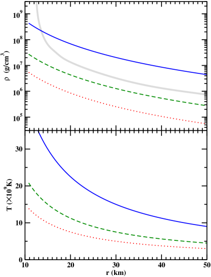
Figure 1: Solid ($S_{100}$ = 0.5), dashed ($S_{100}$ = 1), and dotted ($S_{100}$=1.5) lines corresponds to matter density profiles (upper panel), and temperature profiles (lower panel) based on heuristic description. The thick band in the upper panel is matter density profile from numerical supernova models for $t_{PB}\approx 4$ s (taken from ref [13]).

2.2 Neutrino Fluxes and Luminosities

We adopt the prescription in Ref. [14] for the neutrino fluxes. If we take the density of particles to be $\rho$, the number of particles that go through an expanding surface of radius $r$ per unit time is

$$\frac{dN}{dt}=\rho\frac{dV}{dt}=4\pi r^{2}\rho\frac{dr}{dt},$$ (9)

where $N$ is the total number of particles and $V=4\pi r^{3}$. Assuming a Fermi-Dirac distribution function for the neutrino number densities, ignoring neutrino mass in comparison to its energy, and taking the particle velocity to be $c$, Eq. (9) gives for the flux of neutrinos emitted from the neutrinosphere as

$$d\phi_{\nu} = \frac{d^{2}\phi_{\nu}}{dE_{\nu}d\Omega_{\nu}}dE_{\nu}d\Omega_{\nu}$$ (10)

$$= \frac{1}{8\pi^{3}}\frac{c}{(\hbar c)^{3}}\frac{E^{2}_{\nu}dE_{\nu}}{1+\exp[(E_{\nu}-\mu_{\nu})/kT_{\nu}]}d\Omega_{\nu},$$

where $\mu_{\nu}$ is the neutrino chemical potential. Choosing the z-direction as the vector that connects the point where the flux is to be calculated (with radial position $r$) to the center of the neutron star, one sees that the azimuthal symmetry still holds, but the polar angle is bounded by the finite size of the neutrinosphere. Thus

$$\int d\Omega_{\nu}=2\pi(1-\cos\theta_{0}),$$ (11)

where

$$\cos\theta_{0}=\sqrt{1-\frac{R^{2}_{\nu}}{r^{2}}}\approx 1-\frac{R^{2}_{\nu}}{2r^{2}}$$ (12)

with $R_{\nu}$ being the radius of the neutrinosphere. Within this approximation one then obtains the differential neutrino flux as

$$\frac{d\phi_{\nu}}{dE_{\nu}}=\frac{1}{8\pi^{2}}\frac{c}{(\hbar c)^{3}}\frac{R^{2}_{\nu}}{r^{2}}\frac{E^{2}_{\nu}}{1+\exp[(E_{\nu}-\mu_{\nu})/kT_{\nu}]}.$$ (13)

Using similar reasoning one can write an expression for the neutrino luminosity. Replacing $N$ in Eq. (9) by the total energy and the matter density $\rho$ by the energy density one can write down

$$L_{\nu}=4\pi r^{2}c\frac{1}{2\pi\hbar^{2}}\int\frac{E_{\nu}d^{3}{\bf p}_{\nu}}{1+\exp[(E_{\nu}-\mu_{\nu})/kT_{\nu}]}.$$ (14)

Again ignoring the neutrino mass as compared to its energy and using Eqs. (11) and (12) to do the angular integration we obtain

$$L_{\nu}=\frac{cR_{\nu}^{2}}{2\pi(\hbar c)^{3}}(kT_{\nu})^{4}F_{3}(\eta),$$ (15)

where $\eta=\mu_{\nu}/kT_{\nu}$ and $F_{3}(\eta)$ is the relativistic Fermi integral

$$F_{3}(\eta)=\int_{0}^{\infty}\frac{x^{3}}{1+\exp(x-\eta)}dx.$$ (16)

In our calculations we take $\eta=0$ and use the value $F_{3}(0)=7\pi^{4}/120$. Often it is convenient to express the neutrinosphere radius in terms of the neutrino luminosity. Rewriting $R_{\nu}$ in terms of $L_{\nu}$ and inserting it into Eq. (13) we get

$$\frac{d\phi_{\nu}}{dE_{\nu}}=\frac{1}{4\pi r^{2}}\frac{L_{\nu}}{(kT_{\nu})^{4}F_{3}(\eta)}\left(\frac{E^{2}_{\nu}}{1+\exp[(E_{\nu}-\mu_{\nu})/kT_{\nu}]}\right).$$ (17)

2.3 Reaction Rates

The dominant reactions that control the $n/p$ ratio is the capture reactions on free nucleons

$$\nu_{e}+{\rm n}\rightleftharpoons{\rm p}+e^{-},$$ (18)

and

$$\bar{\nu}_{e}+{\rm p}\rightleftharpoons{\rm n}+e^{+}.$$ (19)

We take the cross sections for the forward reactions to be [16]

$$\sigma_{\nu_{e}}(E_{\nu_{e}})\approx 9.6\times 10^{-44}\left(\frac{E_{\nu_{e}}+\Delta_{np}}{\rm MeV}\right)^{2}{\rm cm}^{2},$$ (20)

and

$$\sigma_{\bar{\nu_{e}}}(E_{\bar{\nu_{e}}})\approx 9.6\times 10^{-44}\left(\frac{E_{{\bar{\nu}_{e}}}-\Delta_{np}}{\rm MeV}\right)^{2}{\rm cm}^{2},$$ (21)

where $\Delta_{np}\approx 1.293$ MeV is the neutron proton mass difference. For simplicity we ignored weak magnetism and recoil corrections, which may be important [20]. These corrections cancel for the former cross section, but add for the latter one. The rates of these reactions can be written as [21]

$$\lambda=\int\sigma(E)_{\nu}\frac{d\phi_{\nu}}{dE_{\nu}}dE_{\nu}.$$ (22)

To calculate the neutrino capture rates on nuclei one needs to include all possible transitions from the parent to the daughter nucleus, including not only the allowed transitions, but also transitions to the isobaric analog states, Gamow-Teller resonance states, transitions into continuum, as well as forbidden transitions. Aspects of such calculations are discussed in Refs. [22] and [23] (see also [24]). Careful input of such reaction rates in supernova simulations is especially crucial to assess the possibility of core-collapse supernovae as a site of the r-process nucleosynthesis [11, 25].

Because of their charged-current interaction electron neutrinos may play a role in reheating the stalled shock as well as regulating the neutron-to-proton ratio. In contrast, since the energies of the muon and tau neutrinos and antineutrinos produced are too low to produce charged leptons, these neutrinos interact only with the neutral-current interactions. Recently significant attention was directed towards understanding the $\nu_{\mu}$ and $\nu_{\tau}$ spectra formation. Neutrinos remain in local thermal equilibrium as long as they can participate in reactions that allow exchange of energy and neutrino pair creation or annihilation. It turns out that the neutrino bremsstrahlung process

$$N+N\leftrightarrow N+N+\nu+\bar{\nu}$$ (23)

is more effective than the annihilation process $\nu+\bar{\nu}\leftrightarrow e^{+}+e^{-}$ at equilibrating neutrino number density [26]. (However the neutrino-neutrino annihilation process $\nu_{e}+\bar{\nu}_{e}\leftrightarrow\nu_{\mu}+\bar{\nu}_{\mu}$ is one of the primary sources of muon and tau neutrinos [28]). The impact of the neutrino bremsstrahlung process on equilibrating the energy spectra seems to be comparable to that of

$$\nu_{\mu,\tau}+e^{-}\rightarrow\nu_{\mu,\tau}+e^{-}.$$ (24)

The most effective process to exchange energy is [27]

$$\nu+N+N\rightarrow N+N+\nu,$$ (25)

which dominates the neutrino spectra formation. Finally recoil corrections to the $\nu N$ interactions are very important in the formation of the $\nu_{\mu}$ and $\nu_{\tau}$ spectra as they permit energy exchange [29].

2.4 Electron Fraction

The electron fraction, $Y_{e}$, is the net number of electrons (number of electrons minus the number of positrons) per baryon:

$$Y_{e}=(n_{e^{-}}-n_{e^{+}})/n_{B},$$ (26)

where $n_{e^{-}}$, $n_{e^{+}}$, and $n_{B}$ are number densities of electrons, positrons, and baryons, respectively. Introducing $N_{j}$, number of species of kind $j$ per unit volume, and $A_{j}$, atomic weight of the $j$-th species, one can write down expressions for the mass fraction, $X_{j}$

$$X_{j}=\frac{N_{j}A_{j}}{\sum_{i}N_{i}A_{i}},$$ (27)

and the number abundance relative to baryons, $Y_{j}$,

$$Y_{j}=\frac{X_{j}}{A_{j}}=\frac{N_{j}}{\sum_{i}N_{i}A_{i}}.$$ (28)

The electron fraction defined in Eq. (26) can then be rewritten as

$$Y_{e} = \sum_{i}Z_{i}Y_{i}=\sum_{i}\left(\frac{Z_{i}}{A_{i}}\right)X_{i}$$ (29)

$$= X_{p}+\frac{1}{2}X_{\alpha}+\sum_{h}\left(\frac{Z_{h}}{A_{h}}\right)X_{h},$$

where $Z_{i}$ is the charge of the species of kind $i$, and the mass fractions of protons, $X_{p}$, alpha particles, $X_{\alpha}$, and heavier nuclei (“metals”), $X_{h}$, are explicitly indicated.

The rate of change of the number of protons can be expressed as

$$\frac{dN_{p}}{dt}=-(\lambda_{\bar{\nu}_{e}}+\lambda_{e^{-}})N_{p}+(\lambda_{\nu_{e}}+\lambda_{e^{+}})N_{n},$$ (30)

where $\lambda_{\nu_{e}}$ and $\lambda_{e^{-}}$ are the rates of the forward and backward reactions in Eq. (18) and $\lambda_{\bar{\nu}_{e}}$ and $\lambda_{e^{+}}$ are the rates of the forward and backward reactions in Eq. (19). Since the quantity $\sum_{i}N_{i}A_{i}$ does not change with neutrino interactions, one can rewrite Eq. (30) in terms of mass fractions

$$\frac{dX_{p}}{dt}=-(\lambda_{\bar{\nu}_{e}}+\lambda_{e^{-}})X_{p}+(\lambda_{\nu_{e}}+\lambda_{e^{+}})X_{n}.$$ (31)

In the hot bubble the rates are usually expressed in terms of the radial velocity field, $v(r)$, above the neutron star, i.e. $dY/dt=v(r)[dY/dr]$. A careful study of the influence of nuclear composition on $Y_{e}$ in the post-core bounce supernova environment is given in Ref. [30] to which we refer the reader for further details.

If no heavy nuclei are present we can write

$$Y_{e}=X_{p}+\frac{1}{2}X_{\alpha}.$$ (32)

Because of the very large binding energy, the rate of alpha particle interactions with neutrinos is nearly zero and we can write $dY_{e}/dt=dX_{p}/dt$. Using the constraint $X_{p}+X_{n}+X_{\alpha}=1$ and Eq. (32), Eq. (31) can be rewritten as

$$\frac{dY_{e}}{dt}=\lambda_{n}-(\lambda_{p}+\lambda_{n})Y_{e}+\frac{1}{2}(\lambda_{p}-\lambda_{n})X_{\alpha},$$ (33)

where we introduced the total proton loss rate $\lambda_{p}=\lambda_{\bar{\nu}_{e}}+\lambda_{e^{-}}$ and the total neutron loss rate $\lambda_{n}=\lambda_{\nu_{e}}+\lambda_{e^{+}}$. It has been shown that when the rates of these processes are rapid as compared to the outflow rate a “weak chemical equilibrium” is established [13]. The weak freeze-out radius is defined to be where the neutron-to-proton conversion rate is less than the outflow rate of the material. If the plasma reaches a weak equilibrium stage then $Y_{e}$ is no longer changing: $dY_{e}/dt=0$. From Eq. (33) one can write the equilibrium value of the electron fraction

$$Y_{e}=\frac{\lambda_{n}}{\lambda_{p}+\lambda_{n}}+\frac{1}{2}\frac{\lambda_{p}-\lambda_{n}}{\lambda_{p}+\lambda_{n}}X_{\alpha}.$$ (34)

Different flavors of neutrinos decouple at different radii. Since $\nu_{\mu}$ and $\nu_{\tau}$ (and their antiparticles) interact with the ordinary matter only with the neutral current interactions, they decouple deeper in the core and have a large average energy. Electron neutrinos and antineutrinos have additional charged-current interactions with neutrons and protons respectively. Since in the supernova environment there are more neutrons, electron antineutrinos decouple after $\nu_{\mu}$’s and $\nu_{\tau}$’s, but before electron neutrinos. Consequently one has a hierarchy of average neutrino energies:

$$\langle E_{\nu_{e}}\rangle\leq\langle E_{\bar{\nu}_{e}}\rangle\leq\langle E_{\nu_{x},\bar{\nu}_{x}}\rangle,$$ (35)

where $\nu_{x}$ stands for any combination of $\nu_{\mu}$’s and $\nu_{\tau}$’s. However a more complete description of the microphysics suggests that this hierarchy of average energies may not be very pronounced [29, 28, 31]. This microphysics is dominated by the inelastic neutrino-nucleon interactions discussed in Section 2.3.

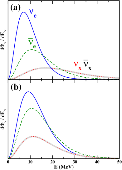
Figure 2: Initial differential neutrino fluxes in arbitrary units. Solid, dashed, dotted, and thick lines correspond to the distributions of $\nu_{e}$, $\bar{\nu}_{e}$, $\nu_{x}$, and $\bar{\nu}_{x}$. a) Fluxes with $\langle E_{\nu_{e}}\rangle=10$ MeV, $\langle E_{\bar{\nu}_{e}}\rangle=15$ MeV, and $\langle E_{\nu_{x},\bar{\nu}_{x}}\rangle=24$ MeV. Neutrino and antineutrino luminosities are taken to be equal for all flavors. Distributions of $\nu_{x}$,$\bar{\nu}_{x}$ have much longer tails up to 100 MeV not shown in the figure. b) Fluxes with $\langle E_{\nu_{e}}\rangle=13$ MeV, $\langle E_{\bar{\nu}_{e}}\rangle=15$ MeV, and $\langle E_{\nu_{x},\bar{\nu}_{x}}\rangle=16$ MeV. $\nu_{e}$ and $\bar{\nu}_{e}$ luminosities are taken to be equal. Luminosities of other flavors are taken to be half of the $\nu_{e}$ and $\bar{\nu}_{e}$ luminosities.

In Figure 2, we present initial differential neutrino fluxes. In the upper panel the typical post-bounce neutrino energies are taken as the representative values of $\langle E_{\nu_{e}}\rangle=10$ MeV, $\langle E_{\bar{\nu}_{e}}\rangle=15$ MeV, and $\langle E_{\nu_{x},\bar{\nu}_{x}}\rangle=24$ MeV. (Average neutrino temperature for each flavor can be calculated using the relation: $T_{\nu}=\langle E_{\nu}\rangle/3.151$). Here neutrino and antineutrino luminosities are taken to be equal for all flavors. We express the neutrino luminosities in more convenient units of $10^{51}\,{\rm ergs}\,{\rm s}^{-1}$. Equal luminosities of $L^{51}_{\nu}=1$ is typically a good approximation for the neutrino-driven wind epoch. However, at earlier epochs, $\nu_{e}$ and $\bar{\nu}_{e}$ luminosities can be as large as $L^{51}_{\nu}=10$. Except, through the neutronization burst, for few milliseconds ${\nu}_{e}$ luminosity can reach values of $L^{51}_{\nu}=100$, an order of magnitude larger than $\bar{\nu}_{e}$ during the same period. In the lower panel of Figure 2 we examine a less-pronounced hierarchy of neutrino energies. Here we adopt the representative values of $\langle E_{\nu_{e}}\rangle=13$ MeV, $\langle E_{\bar{\nu}_{e}}\rangle=15$ MeV, and $\langle E_{\nu_{x},\bar{\nu}_{x}}\rangle=16$ MeV. Here the luminosities of $\nu_{x}$ and $\bar{\nu}_{x}$ are taken to be the half of the value of the equal luminosities of $\nu_{e}$ and $\bar{\nu}_{e}$.

In our calculations in Section 4, we adapt these initial distributions of $\nu_{e}$, $\bar{\nu}_{e}$, $\nu_{x}$ and $\bar{\nu}_{x}$ at neutrinosphere, $R_{\nu}$=10 km, with the indicated luminosities and follow the evolution of differential neutrino fluxes (number of neutrinos per unit energy per unit volume).

2.5 Alpha Effect

At high temperatures alpha particles are absent and the second term in Eq. (34) can be dropped. In the region just below where the alpha particles are formed approximately one second after the bounce, the temperature is less then $\sim 1$ MeV. Here both the electron and positron capture rates are very small and $Y_{e}$ can be approximated as

$$Y_{e}^{(0)}=\frac{1}{1+\lambda_{\bar{\nu}_{e}}/\lambda_{\nu_{e}}}.$$ (36)

As the alpha particle mass fraction increases (when $T_{9}$ drops below 8) free nucleons get bound in alphas and, because of the large binding energy of the alpha particle, cease interacting with neutrinos. This phenomenon is called “alpha effect” [22]. Using Eq. (36) one can rewrite Eq. (34) as

$$Y_{e}=Y_{e}^{(0)}+\left(\frac{1}{2}-Y_{e}^{(0)}\right)X_{\alpha}.$$ (37)

Hence if the initial electron fraction is small ($Y_{e}^{(0)}<1/2$) the alpha effect increases the value of $Y_{e}$. Since higher $Y_{e}$ implies fewer free neutrons, the alpha-effect negatively impacts r-process nucleosynthesis [25].

Neutrino oscillations, since they can swap energies of different flavors, can effect the energy-dependent rates in Eqs. (36) and (37), changing the electron fraction. Indeed, transformations between active flavors heat up $\nu_{e}$’s and increase $\lambda_{\nu_{e}}$, driving the electron fraction to rather large values. Consequently a very large mixing between active neutrino flavors would have prohibited r-process nucleosynthesis in a core-collapse supernova [13, 14].

Actually electron neutrinos radiated from the proto-neutron stars are just too energetic to prevent the alpha effect in most cases. One possibility to reduce $\lambda_{\nu_{e}}$ is to convert active electron neutrinos into sterile ones which do not contribute to this rate. This possibility is explored in references [18], [32] and [33].

3 Neutrino Mixing

Neutrino interactions in matter is a rich subject (for a brief review see Ref. [34]). While neutrinos are produced through weak interactions in flavor eigenstates, they propagate in mass eigenstates. Mixing angles correspond to rotations describing unitary connection between two bases:

$$\left(\begin{array}[]{c}\nu_{e}\\ \nu_{\mu}\\ \nu_{\tau}\end{array}\right)=U_{\alpha i}\left(\begin{array}[]{c}\nu_{1}\\ e^{i\phi_{1}}\nu_{2}\\ e^{i\phi_{2}}\nu_{3}\end{array}\right).$$ (38)

In our discussion, we follow the notation in Ref. [35] and denote the neutrino mixing matrix by $U_{\alpha i}$ where $\alpha$ denotes the flavor index and $i$ denotes the mass index:

$$U_{\alpha i}=\left(\matrix{1&0&0\cr 0&C_{23}&S_{23}\cr 0&-S_{23}&C_{23}}\right)\left(\matrix{C_{13}&0&S_{13}^{\ast}\cr 0&1&0\cr-S_{13}&0&C_{13}}\right)\left(\matrix{C_{12}&S_{12}&0\cr-S_{12}&C_{12}&0\cr 0&0&1}\right).$$ (39)

In Eq. (39) $C_{13}$, etc. is the short-hand notation for $\cos{\theta_{13}}$, etc. The notation $S_{13}^{\ast}$ was used to indicate $(\sin{\theta_{13}})e^{i\phi}$ where $\phi$ is a CP-violating phase. We will ignore this phase in our discussion.

We have compelling evidence supporting non-zero neutrino masses and mixings. Two-flavor solar neutrino solution corresponding to $\theta_{12}\sim\pi/6$ and $\delta m_{12}^{2}\sim 8\times 10^{-5}$ eV² was identified using the recent Sudbury Neutrino Observatory (SNO) results (cf. Refs. [36], [37]). Measurement of anti-neutrinos from nuclear power reactors in Japan by the KamLAND experiment confirmed this solution and improved the limits on the solar mass square difference, $\delta m_{12}^{2}$, significantly [38]. While it is known that the solar neutrino mixing angle is large, but not maximal, the atmospheric mixing angle is large and could be maximal, $\theta_{23}\sim\pi/4$, as shown by the Super-Kamiokande experiment [39]. The latter angle is consistent with the KEK-to-Kamioka oscillation experiment, K2K [40]. The corresponding atmospheric mass square difference is $\delta m_{23}^{2}\sim 3\times 10^{-3}$ eV².

The size of the last mixing angle, $\theta_{13}$ is currently best limited by the combined CHOOZ [41] and Palo Verde [42] reactor experiments and SK atmospheric data. This is due to the null results from the reactor $\bar{\nu}_{e}$ disappearance over the $\delta m_{23}^{2}$ distance scale. The upper bound on this angle from KamLAND and the solar neutrino data gets stronger (especially in the region with small atmospheric mass square difference where CHOOZ reactor bound is relatively weak), and even dominates, as this data get refined [43]. Both measurements of the width of the Z boson and oscillation interpretation of the neutrino data, with the notable exception of the LSND signal [44], favor three generations of light active neutrino species. If LSND is confirmed, the most likely explanation could be the existence of a fourth neutrino (a relatively heavier sterile neutrino) since agreement between KamLAND and combined solar experiments already disfavors the interpretation of the LSND anomaly with CP violation.

In the region above the supernova core density is still high, but steeply decreases. Matter-enhanced oscillations mediated by the solar mass square difference are impossible in the region close to the core which is suitable for the r-process. However, at late neutrino driven epoch baryon density could be low enough to allow resonances through $\delta m_{13}^{2}$, which is comparable to the atmospheric mass square difference. At such late times neutrino flux is expected to be low. We examine prospects of r-process at such environments in the next section.

We describe neutrino mixing within the density matrix formalism [14, 45, 46, 47]. We assume that the electron neutrino mixes with a linear combination of $\mu$ and $\tau$ neutrinos. The neutrino oscillations are mediated by the matter mixing angle for transformation between 1st and 3nd mass eigenstates, $\theta_{13}$, and the corresponding atmospheric mass square difference, $\delta m_{13}^{2}$. The mixing between $\mu$ and $\tau$ neutrino flavors does not have any significant effect on our results as long as total luminosities and corresponding average energies are equal and their mixing is maximal. In this limit, mixing between 2nd and 3nd mass eigenstates, can be rotated away and effectively electron neutrinos oscillates into some linear combination of $\mu$ and $\tau$ neutrinos [48].

In the rest of the paper $\theta$ and $\delta m^{2}$ refer to $\theta_{13}$ and $\delta m_{13}^{2}$. This assumption simplifies the discussion and allows us to write the two-flavor density matrices as

$$\rho=\left(\begin{array}[]{cc}\rho_{ee}&\rho_{ex}\\ \rho_{xe}&\rho_{xx}\end{array}\right)=\frac{1}{2}\left(P_{0}+{\bf P}\cdot{\bf\sigma}\right)$$ (40)

and

$$\bar{\rho}=\left(\begin{array}[]{cc}\bar{\rho}_{ee}&\bar{\rho}_{ex}\\ \bar{\rho}_{xe}&\bar{\rho}_{xx}\end{array}\right)=\frac{1}{2}\left(\bar{P}_{0}+\bar{\bf P}\cdot{\bf\sigma}\right),$$ (41)

where we introduced the polarization vectors for neutrinos and anti-neutrinos, ${\mathbf{P}}_{p}$ and $\bar{{\mathbf{P}}}_{p}$. The diagonal elements in these expressions are initially given by the expression in Eq. (17). Non-diagonal elements are initially zero but may become non-zero during the neutrino evolution.

Equations governing the evolution of neutrinos and antineutrinos can be cast into the forms [49]

$$\partial_{r}{\mathbf{P}}_{p}=\left\{+{\mathbf{\Delta}}_{p}+\sqrt{2}\,G_{\rm F}\left[N_{e}\hat{\bf z}+\int d{\bf q}\left(1-\frac{\bf p.q}{p\>q}\right)({\mathbf{P}_{\bf p}}-{\mathbf{\overline{P}}}_{\bf q})\right]\right\}\times{\mathbf{P}}_{p},$$ (42)

and

$$\partial_{r}{\mathbf{\overline{P}}}_{p}=\left\{-{\mathbf{\Delta}}_{p}+\sqrt{2}\,G_{\rm F}\left[N_{e}\hat{\bf z}+\int d{\bf q}\left(1-\frac{\bf p.q}{p\>q}\right)({\mathbf{P}_{\bf p}}-{\mathbf{\overline{P}}}_{\bf q})\right]\right\}\times{\mathbf{\overline{P}}}_{p},$$

where

$${\mathbf{\Delta}}_{p}=\frac{\delta m^{2}}{2p}(\sin 2\theta{\mathbf{\hat{x}}}-\cos 2\theta{\mathbf{\hat{z}}}),$$ (43)

Integrating Eqs. (42) and (3) exactly in the supernova environment is, at the moment, an unsolved problem. Indeed the exact solutions of these coupled, non-linear differential equations are expected to be very complicated. Instead we adopt the approximation proposed in Ref. [14] and also adopted in Ref. [49]. In this approximation one uses flux-averaged values to obtain

$$\partial_{r}{\mathbf{P}}_{p}=\left(+{\mathbf{\Delta}}_{p}+\sqrt{2}\,G_{\rm F}N_{e}\hat{\bf z}+\sqrt{2}G_{\rm F}F(r)({\mathbf{J}}-{\mathbf{\overline{J}}})\right)\times{\mathbf{P}}_{p}$$ (44)

and

$$\partial_{r}{\mathbf{\overline{P}}}_{p}=\left(-{\mathbf{\Delta}}_{p}+\sqrt{2}\,G_{\rm F}N_{e}\hat{\bf z}+\sqrt{2}G_{\rm F}F(r)({\mathbf{J}}-{\mathbf{\overline{J}}})\right)\times{\mathbf{\overline{P}}}_{p}$$

In these equations ${\mathbf{J}}$ is the polarization integrated over all momentum modes, and $F(r)=\frac{1}{2}[1-(1-R_{\nu}^{2}/r^{2})^{1/2}]$ is the geometrical factor introduced earlier (cf. Eqs. (11) and (12)).

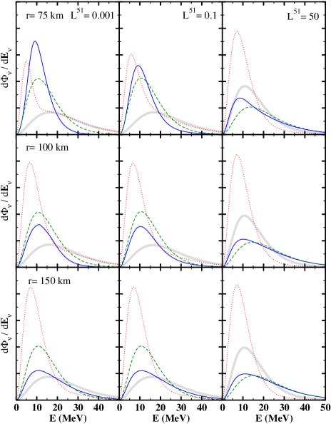
Figure 3: Evolution of differential neutrino fluxes in arbitrary units. Solid, dashed, dotted, and thick lines correspond to the distributions of $\nu_{e}$, $\bar{\nu}_{e}$ $\nu_{\mu}$, and $\bar{\nu}_{\mu}$. In each panel, $1/r^{2}$ dependence is removed. Columns are for $L^{51}$ = 0.001, 0.1, and 50 from left to the right corresponding to very weak, moderate, and very strong neutrino self interaction contributions to the evolution. Rows are calculated at $r=$ 75 km, 100 km, and 150 km showing the evolution of distributions along neutrino path. See text for details.

4 Results and Discussion

In our calculations, we concentrate on the late neutrino-driven wind epoch which is expected to have larger entropy. We adopt $S_{100}$ = 1.5 and the $g_{S}$ = 2, since in this epoch the temperature is too low at later times to have electron-positron pairs to be adequately represented.

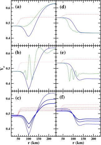
Figure 4: Initial neutrino fluxes and luminosities are taken to be those in Figure 2(a) in the left column and those in Figure 2(b) in the right column. $S_{100}$ is taken to be 1.5. In panels (a) and (b), solid, dashed and dotted lines correspond to the equal luminosities of $L^{51}$ = 0.001, 0.1, and 50 for all flavors, indicating very weak, moderate, and very-strong neutrino self interaction contributions to the evolution. In panels (d), and (e) $\nu_{e}$ and $\bar{\nu}_{e}$ luminosities are taken to be $L^{51}$ = 0.002, 0.2, and 200 (solid, dashed and dotted lines, respectively). In (d) and (e) the luminosities of other flavors are taken to be $L^{51}$ = 0.001, 0.1, and 100 (solid, dashed and dotted lines, respectively). (a, d) Equilibrium electron fraction as a function of the distance from the core with mixing parameters $\theta_{13}\sim\pi/10$ and $\delta m_{13}^{2}\sim 3\times 10^{-3}$ eV². (b, e) Equilibrium $Y_{e}$ as a function of the distance from the core with mixing parameters $\theta_{13}\sim\pi/20$ and $\delta m_{13}^{2}\sim 3\times 10^{-3}$ eV². (c) Same as (b) but the impact of alpha particle formation is included according to the Eq. (34). $Y_{e}$ is shown when $X_{\alpha}$=0, 0.3 and 0.5 (thin, medium and thick lines) for $L^{51}$=0.001 and 50 (solid and dotted sets of lines). (f) Same as (e) but the impact of alpha particle formation is included as in (c). $Y_{e}$ is shown when $X_{\alpha}$=0, 0.3 and 0.5 (thin, medium and thick lines) for $L_{\nu_{e}}^{51}$=0.002 and 200 (solid and dotted sets of lines).

In Figure 3 we present differential neutrino fluxes at several stages of the evolution in order to provide a better understanding of this mechanism. The mixing parameters are chosen as $\theta\sim\pi/10$ and $\delta m^{2}\sim 3\times 10^{-3}$ eV². Solid, dashed, dotted, and thick lines correspond to the distributions of $\nu_{e}$, $\bar{\nu}_{e}$, $\nu_{x}$,and $\bar{\nu}_{x}$. In each panel, $1/r^{2}$ dependence is removed. For this figure the initial distributions are taken as the values given in Figure 2a). Columns are for $L^{51}$ = 0.001, 0.1, and 50 from left to the right corresponding to very weak, moderate, and very strong neutrino self interaction contributions to the evolution. Rows show neutrino flux at $r=$ 75 km, 100 km, and 150 km, exhibiting the evolution of neutrino distributions along the neutrino path. These should be compared to the initial (at $\sim 10$ km) neutrino distributions given in Figure 2a). Electron fractions corresponding to these luminosities are given in the left column of Figure 4.

$\bullet$ First column of Figure 3, $L^{51}$ = 0.001: Initially differential neutrino fluxes for $\nu_{e}$ and $\nu_{x}$ are the same at $\sim$ 20 MeV as seen in Figure 2a). At energies lower than 20 MeV, differential flux of $\nu_{e}$ is higher than that of $\nu_{x}$ whereas at energies higher than 20 MeV the numbers reverse. The transformation starts at the low energy tail of the distributions. As we gradually move to lower densities resonance moves up to higher energies. Until we reach the resonance at 20 MeV the luminosity of $\nu_{e}$’s decreases. At r = 100 km electron neutrinos below 20 MeV are mostly swapped with $\nu_{x}$’s while above 20 MeV there is yet no significant transformation. This point corresponds to the minimum of $\lambda$ of Eq. (22) for neutrinos (after the $1/r^{2}$-dependence is taken out). Since antineutrinos are not transformed $\lambda$ is constant for them. As a results, r $\sim$ 100 km corresponds to a dip in $Y_{e}$ (solid line in figure 4(a)). Since above 20 MeV the initial differential flux of $\nu_{e}$’s is smaller than that of $\nu_{x}$’s, transformations after r $\sim$ 100 km would increase the number of high energy $\nu_{e}$’s. As neutrinos travel to regions further away (r= 150 km, where baryon density is much lower), swapping of high energy tail of the $\nu_{e}$ and $\nu_{x}$ distributions is completed, and $Y_{e}$ approaches to the asymptotic fixed value.

$\bullet$ Second column of Figure 3, $L^{51}$ = 0.1: This column describes the same evolution of neutrinos except that neutrino self-interaction effects play a more pronounced role. The chosen value of the luminosity could be representative of such late times in neutrino-driven wind epoch. Because of the small contributions of the self interactions, resonance region is relatively wider. No dip is observed in $Y_{e}$ (dashed line in figure 4(a)) at r = 100 km because transformation of low and high energy ends of the distributions happen almost simultaneously. There is also small transformation between $\bar{\nu}_{e}$’s and $\bar{\nu}_{x}$’s.

$\bullet$ Third column of Figure 3, $L^{51}$ = 50: This is an extreme case to illustrate the limit at which neutrino self interactions dominate. Swapping of both neutrinos and antineutrinos occur and $Y_{e}$ reaches its equilibrium value rapidly. After the transformation, electron neutrinos and antineutrinos assume similar luminosities and distributions since they are swapped with $\nu_{x}$’s and $\bar{\nu}_{x}$’s. Note that this equilibrium value is again different from 0.5 because of the threshold effects (due to the neutron-proton mass difference) in the reaction cross sections (cf. Eqs. (20) and (21)).

In the left column of Figure 4 initial neutrino fluxes and luminosities are taken to be those in Figure 2(a) and in the right column initial neutrino fluxes and luminosities are taken to be those in Figure 2(b). In Figure 4(a) we present the equilibrium electron fraction, $Y_{e}$, as a function of the distance from the core for the three different cases of neutrino flux, $L^{51}$ = 0.001, 0.1, and 50, each corresponding to one of the columns in Figure 3. In Figure 4(a) we use the same neutrino parameters as in Figure 3. One could argue that the relatively large mixing angle of $\pi/10$ is already disfavored by CHOOZ. To explore the implications of a smaller mixing angle, in Figure 4(b) we show electron fractions calculated with the more realistic mixing parameters $\theta\sim\pi/20$ and $\delta m^{2}\sim 3\times 10^{-3}$ eV². The dip in $Y_{e}$ plot is sharper since resonance region will be much narrower with the smaller mixing angle.

In Figures 4 a) and b), to calculate the equilibrium electron fraction, we ignored possible effects of the alpha particles and used Eq. (36) to evaluate $Y_{e}$. In 4(c), we explore possible effects of alpha particles by using Eq. (34) to calculate $Y_{e}$ for three different values of $X_{\alpha}$. The “alpha effect” is manifest: as $X_{\alpha}$ gets larger, it pulls the value of the electron fraction closer to 0.5.

In the right column of Figure 4 initial neutrino fluxes and luminosities are taken as the generic “almost equal” energies and different luminosities case shown in Figure 2(b). It is immediately obvious that the situation is markedly different in this case. Even though the initial $\nu_{e}$ and $\bar{\nu}_{e}$ spectra are about the same (cf. Figure 2(b)), $Y_{e}$ initially is greater than $0.5$ because of the effect of the neutron-proton mass difference in Eqs. (20 and (21). When the effects of the neutrino self-interaction terms are minimal (the low-luminosity case indicated by the solid lines in (d) and (e)), after $\nu_{e}$’s and $\nu_{x}$’s swap $\nu_{e}$ luminosity decreases significantly causing a big drop in the value of $Y_{e}$. When the effects of the self-interaction terms are dominant (the high luminosity cases indicated by the dotted lines in (d) and (e)), all flavors swap and the electron fraction eventually reaches to the asymptotic values. The impact of alpha formation, when the hierarchy of average neutrino energies is less pronounced, is presented in Figure 4(f).

5 Conclusions

In this article we investigated conditions for the r-process nucleosynthesis at late neutrino-driven wind epoch in a core-collapse supernova. We considered the region where the matter-enhanced neutrino transformation is driven by $\delta m_{13}^{2}$, which we took to be comparable to the mass difference observed in the atmospheric neutrino oscillations.

We found that, when initial luminosities are taken to be equal with a pronounced hierarchy of neutrino energies, the asymptotic value (at large distances from the core) of the electron fraction always exceeds 0.5, hindering the r-process nucleosynthesis. In this case we found that neutrino self-interactions decrease the electron fraction. In general these self-interaction terms, unlike the MSW effect, tend to transform both neutrinos and antineutrinos. Hence one expects that when the self interaction terms are dominant (e.g when the neutrino luminosities are very large) the electron fraction would reach to the value of 0.5. However we showed that, because of the threshold effects in the neutrino interactions, electron fraction exceeds 0.5 even when the background neutrinos are numerous. Clearly these conditions are not favorable for the r-process nucleosynthesis. We also found that, when background effects are small, with the parameters we adopted for baryon density and neutrino mixing there exists a region around 100 km in which electron fraction is smaller than 0.5. Even in this region alpha effect pulls the value of the electron fraction closer to 0.5. Although the conditions are favorable, the r-process in this region could not contribute reasonable quantities of elements since the baryon density is rather low.

In contrast, when the initial luminosities of the $\nu_{e}$’s and $\bar{\nu}_{e}$’s are taken to be twice of the other flavors with a much less pronounced neutrino hierarchy, we found that the asymptotic electron fraction is less than 0.5 when neutrino self-interactions are negligible. However, once again the baryon density is low and r-process in this asymptotic region is likely to produce insignificant quantities. When neutrino self-interactions are dominant the asymptotic electron fraction shows the same behavior as the first generic case (with a pronounced hierarchy of neutrino energies and equal luminosities) we considered.

It is not surprising that the two cases are markedly different for low neutrino luminosities (late times). If all the initial average neutrino energies and luminosities were the same neutrino oscillations would clearly have no impact. Our analysis highlights the significance of having a precise knowledge of the muon and tau neutrino spectra and luminosities in assessing core-collapse supernovae as a site of r-process nucleosynthesis. In both of the two generic, but markedly different, cases we studied we found that neutrino self-interactions are crucial in setting the value of the electron-fraction to be rather large. We should emphasize that our treatment of the neutrino self-interactions in Eqs. (44) and (3) is an approximation using flux-averaged values. Hence an exact treatment of the neutrino self-interactions remains to be the key issue in the proper description of the neutrino transport in core-collapse supernovae.

References

References

- [1] S.E. Woosley, A. Heger, and T.A. Weaver, Rev. Mod. Phys. 74 (2002) 1015.
- [2] R. Buras, M. Rampp, H. T. Janka and K. Kifonidis, Phys. Rev. Lett. 90 (2003) 241101 [arXiv:astro-ph/0303171].
- [3] A. Mezzacappa, arXiv:astro-ph/0410085.
- [4] Y. Z. Qian, Prog. Part. Nucl. Phys. 50 (2003) 153 [arXiv:astro-ph/0301422].
- [5] E.M. Burbidge, G.R. Burbidge, W.A. Fowler, and F. Hoyle, Rev. Mod. Phys. 29 (1957) 29.
- [6] S. E. Woosley, J. R. Wilson, G. J. Mathews, R. D. Hoffman and B. S. Meyer, Astrophys. J. 433 (1994) 229.
- [7] K. Takahashi, J. Witti, and H.-T. Janka, Astron. Astrophys. 286 (1994) 857.
- [8] S. Wanajo, T. Kajino, G. J. Mathews and K. Otsuki, Astrophys. J. 554 (2001) 578 [arXiv:astro-ph/0102261].
- [9] Y. Z. Qian, P. Vogel and G. J. Wasserburg, Astrophys. J. 494 (1998) 285 [arXiv:astro-ph/9706120].
- [10] S. Rosswog, M. Liebendoerfer, F. K. Thielemann, M. B. Davies, W. Benz and T. Piran, Astronom. Astrophys. 341 (1999) 499 [arXiv:astro-ph/9811367].
- [11] A. B. Balantekin and G. M. Fuller, J. Phys. G 29 (2003) 2513 [arXiv:astro-ph/0309519].
- [12] H. A. Bethe and J. R. Wilson, Astrophys. J. 295 (1985) 14.
- [13] Y. Z. Qian, G. M. Fuller, G. J. Mathews, R. Mayle, J. R. Wilson and S. E. Woosley, Phys. Rev. Lett. 71 (1993) 1965.
- [14] Y. Z. Qian and G. M. Fuller, Phys. Rev. D 51 (1995) 1479 [arXiv:astro-ph/9406073].
- [15] J. Pantaleone, Phys. Lett. B 342 (1995) 250 [arXiv:astro-ph/9405008].
- [16] Y. Z. Qian and G. M. Fuller, Phys. Rev. D 52 (1995) 656 [arXiv:astro-ph/9502080].
- [17] Y. Z. Qian and S. E. Woosley, Astrophys. J. 471 (1996) 331 [arXiv:astro-ph/9611094].
- [18] G. C. McLaughlin, J. M. Fetter, A. B. Balantekin and G. M. Fuller, Phys. Rev. C 59 (1999) 2873 [arXiv:astro-ph/9902106].
- [19] H. A. Bethe, Astrophys. J. 412 (1993) 192.
- [20] C. J. Horowitz and G. Li, Phys. Rev. Lett. 82 (1999) 5198 [arXiv:astro-ph/9904171]; C. J. Horowitz, Phys. Rev. D 65 (2002) 043001 [arXiv:astro-ph/0109209]; C. J. Horowitz and M. A. Perez-Garcia, Phys. Rev. C 68 (2003) 025803 [arXiv:astro-ph/0305138].
- [21] G. M. Fuller, W. A. Fowler and M. J. Newman, Astrophys. J. 252 (1982) 715.
- [22] G. M. Fuller and B. S. Meyer, Astrophys. J. 453 (1995) 792.
- [23] G. C. McLaughlin and G. M. Fuller, Astrophys. J. 455 (1995) 202.
- [24] C. Volpe, arXiv:hep-ph/0409249.
- [25] B. S. Meyer, G. C. McLaughlin and G. M. Fuller, Phys. Rev. C 58 (1998) 3696 [arXiv:astro-ph/9809242].
- [26] H. Suzuki, in Proc. International Symp. on Neutrino Astrophysics, Eds. Y. Suzuki and K. Nakamura (Tokyo: Universal Academy Press, 1993).
- [27] S. Hannestad and G. Raffelt, Astrophys. J. 507 (1998) 339 [arXiv:astro-ph/9711132].
- [28] R. Buras, H. T. Janka, M. T. Keil, G. G. Raffelt and M. Rampp, Astrophys. J. 587 (2003) 320 [arXiv:astro-ph/0205006].
- [29] G. G. Raffelt, Astrophys. J. 561 (2001) 890 [arXiv:astro-ph/0105250].
- [30] G. C. McLaughlin, G. M. Fuller and J. R. Wilson, Astrophys. J. 472 (1996) 440 [arXiv:astro-ph/9701114].
- [31] M. T. Keil, G. G. Raffelt and H. T. Janka, Astrophys. J. 590 (2003) 971 [arXiv:astro-ph/0208035].
- [32] D. O. Caldwell, G. M. Fuller and Y. Z. Qian, Phys. Rev. D 61 (2000) 123005 [arXiv:astro-ph/9910175].
- [33] J. Fetter, G. C. McLaughlin, A. B. Balantekin and G. M. Fuller, Astropart. Phys. 18 (2003) 433 [arXiv:hep-ph/0205029].
- [34] A. B. Balantekin, Phys. Rept. 315 (1999) 123 [arXiv:hep-ph/9808281].
- [35] A. B. Balantekin and H. Yuksel, J. Phys. G 29, 665 (2003) [arXiv:hep-ph/0301072].
- [36] S. N. Ahmed et al. [SNO Collaboration], Phys. Rev. Lett. 92, 181301 (2004) [arXiv:nucl-ex/0309004].
- [37] A. B. Balantekin and H. Yuksel, Phys. Rev. D 68, 113002 (2003) [arXiv:hep-ph/0309079].
- [38] T. Araki et al. [KamLAND Collaboration], arXiv:hep-ex/0406035.
- [39] Y. Ashie et al. [Super-Kamiokande Collaboration], Phys. Rev. Lett. 93, 101801 (2004) [arXiv:hep-ex/0404034].
- [40] M. H. Ahn et al. [K2K Collaboration], Phys. Rev. Lett. 90, 041801 (2003) [arXiv:hep-ex/0212007].
- [41] M. Apollonio et al., Eur. Phys. J. C 27 (2003) 331 [arXiv:hep-ex/0301017].
- [42] F. Boehm et al., Phys. Rev. D 64 (2001) 112001 [arXiv:hep-ex/0107009].
- [43] A. B. Balantekin, V. Barger, D. Marfatia, S. Pakvasa and H. Yuksel, arXiv:hep-ph/0405019.
- [44] A. Aguilar et al. [LSND Collaboration], Phys. Rev. D 64 (2001) 112007 [arXiv:hep-ex/0104049].
- [45] G. Sigl and G. Raffelt, Nucl. Phys. B 406 (1993) 423.
- [46] G. Raffelt, G. Sigl and L. Stodolsky, Phys. Rev. Lett. 70 (1993) 2363 [arXiv:hep-ph/9209276].
- [47] F. N. Loreti and A. B. Balantekin, Phys. Rev. D 50 (1994) 4762 [arXiv:nucl-th/9406003].
- [48] A. B. Balantekin and G. M. Fuller, Phys. Lett. B 471 (1999) 195 [arXiv:hep-ph/9908465].
- [49] S. Pastor and G. Raffelt, Phys. Rev. Lett. 89 (2002) 191101 [arXiv:astro-ph/0207281]; S. Pastor, G. G. Raffelt and D. V. Semikoz, Phys. Rev. D 65 (2002) 053011 [arXiv:hep-ph/0109035].