The Absorption Spectrum of High-Density Stellar Ejecta in the Line-of-Sight to Eta Carinae

Abstract

Using the high dispersion NUV mode of the Space Telescope Imaging Spectrograph (STIS) aboard the Hubble Space Telescope (HST) to observe Eta Carinae, we have resolved and identified over 500 sharp, circumstellar absorption lines of iron-group singly-ionized and neutral elements with $\approx$20 velocity components ranging from $-$146 km s^-1 to $-$585 km s^-1. These lines are from transitions originating from ground and metastable levels as high as 40,000 cm^-1 above ground. The absorbing material is located either in dense inhomogeneities in the stellar wind, the warm circumstellar gas immediately in the vicinity of Eta Carinae, or within the cooler foreground lobe of the Homunculus. We have used classical curve-of-growth analysis to derive atomic level populations for Fe II at $-$146 km s^-1 and for Ti II at $-$513 km s^-1. These populations, plus photoionization and statistical equilibrium modeling, provide electron temperatures, T_e, densities, n_H, and constraints on distances from the stellar source, r. For the $-$146 km s^-1 component, we derive T_e = 6400 K, n${}_{\mathrm{H}}\geq$ 10${}^{7}-$ 10⁸ cm^-3, and d $\approx$ 1300 AU. For the $-$513 km s^-1 component, we find a much cooler temperature, T_e= 760 K, with n${}_{\mathrm{H}}\geq$ 10⁷ cm^-3, we estimate d$\approx$ 10,000 AU. The large distances for these two components place the absorptions in the vicinity of identifiable ejecta from historical events, not near or in the dense wind of $\eta\ Car$. Further analysis, in parallel with obtaining improved experimental and theoretical atomic data, is underway to determine what physical mechanisms and elemental abundances can explain the large number of strong circumstellar absorption features in the spectrum of $\eta\ Car$.

1 Introduction

Eta Carinae ($\eta\ Car$) has been an enigma since the Great Outburst in the 1840’s (Davidson & Humphreys 1999). The 100+ M_☉ star, located at a distance $\sim$2300 pc (Meaburn 1999), with $\sim$10^6.7L_☉ and a very large mass loss rate of $\sim$10^-3M_☉y^-1 is surrounded by a dusty, expanding double-lobed nebular complex known as the Homunculus. Smith et al. (2003) using infrared images estimated that the Homunculus may contain 12 M_☉ of material, most having been ejected since the Great Outburst. Because of its recent activity, proximity, and brightness, $\eta\ Car$ offers a unique opportunity to study mass loss processes of a massive star in considerable detail. Since massive Population III stars are thought to have been abundant in the Early Universe (Heger & Woosley 2003), the nebulosities of $\eta\ Car$ may provide fundamental clues to how extensive mass loss in the last stages of evolution in extremely massive stars, both now and in the Early Universe, enriches the interstellar medium in processed elements.

The observations described herein clearly indicate a rich circumstellar absorption spectrum for the ejecta of $\eta\ Car$. These narrow, interstellar-like features are seen in roughly 20 components with heliocentric velocities from $-$146 to $-$584 km s^-1. The spectral lines of this absorption complex cannot be interstellar and arise in gas at much higher densities (n $\approx$ 10⁷ cm^-3) than those of the multiple interstellar components seen from $+$100 to $-$50 km s^-1 toward other stars in the Carina association (Walborn et al. 2002). The interstellar lines, typifying densities n $\leq$ 10⁴ cm^-3, are formed in the foreground, much lower density H II region gas and interstellar clouds along the line-of-sight to $\eta\ Car$.

2 Observations and Data Reduction

Observations were obtained with the HST/STIS using the E230H grating and the $0\,\farcs 2\times 0\,\farcs 09$ aperture, providing a spectral resolving power of R$\sim$114,000 in the near UV. The HST high spatial resolution, about $0\,\farcs 03$, provides critical separation of the stellar emission from dust-scattered starlight and nebular emission within the Homunculus. The chaotic nature of the expanding ejecta within the Homunculus, the extended wind of the central source and the many emission nebulosities, lead to a velocity-smeared spectrum for spatial scales exceeding $0\,\farcs 1$. These two-dimensional STIS spectral images were acquired under STIS GTO program 9242 on October 1, 2001 (E230H, 2385 to 2940 Å) and GO program 9083 on January 20, 2002 (E230H, 2885 to 3160 Å). Data reduction was performed with the CALSTIS software (Lindler 1999) developed at NASA/GSFC.

3 Analysis

The STIS spectrum of $\eta\ Car$ displays sharp circumstellar and interstellar (IS) lines formed along the line-of-sight (Figure 1). Walborn et al. (2002) identified multiple IS components in the direction of four association stars (including HDE 303308 and CPD $-$59$\arcdeg$2603), ranging in velocity from $+$127 to $-$388 km s^-1. The strongest IS lines, all arising from levels within the ground configuration of the observed species with velocities ranging from $+$100 to $-$50 km s^-1, are also present in the $\eta\ Car$ spectrum. Unique to the $\eta\ Car$ spectrum are absorption lines at $-$146 km s^-1 and the complex circumstellar absorptions between $-$385 to $-$585 km s^-1 coming from a wide range of metastable levels, up to 40,000 cm^-1, in neutral and singly ionized species. Because of the high level of excitation, these absorptions imply densities far above what is expected in the normal ISM. In Figure 2, absorption line profiles are plotted from $-$100 to $-$570 km s^-1 for selected lines of various species. The slowly varying stellar flux is normalized to facilitate the comparison. Two velocity components are readily apparent: one at $-$146 km s^-1 and another at $-$513 km s^-1. In what follows, we will devote our analysis to Fe II and Ti II, respectively, in these two velocity components since they are fairly isolated with minimal contamination by absorption from adjacent components.

The two absorption components at $-$146 and $-$513 km s^-1  are easily distinguishable by their very different characteristic widths and by the range in originating energy levels. The relatively broad component at $-$146 km s^-1, observed in lines of Mg II, Cr II, Fe II, Mn II, Ni II and Co II, originates from a wide range of energy levels. In Figure 2, the $-$146 km s^-1 component is present in Fe II $\lambda\lambda$2715, 2756, both lines arising from a level 7955 cm^-1 above ground. It is significantly broader than the multiple, blended components between $-$385 and $-$585 km s^-1. This component, with identified lines originating from energy levels up to 40,000 cm^-1(nearly 5 eV above ground!), is more excited than the higher velocity components.

The velocity component at $-$513 km s^-1 is observed in lines of both neutral and singly ionized species as in Fe I $\lambda$2995, V II $\lambda$3111 and Ti II $\lambda$3088 (Figure 2). While we have identified weak Fe I lines originating from levels as high as 7400 cm^-1, nearly all lines originate from much lower levels. The V II absorption lines originate from levels ranging up to 3200 cm^-1($\sim$0.4 eV above ground). So far, only upper limits have been found for V II in the interstellar medium (Cardelli 1994; Snow, Weiler & Oegerle 1984; Welty et al. 1992), where these results imply vanadium is at least thirty times under abundant compared to solar values. In the $-$513 km s^-1 absorption component in the spectrum of $\eta\ Car$, we have unambiguously detected over twenty strong absorption lines of V II. The difference in ionization and the relative level populations between the $-$146 and the $-$513 km s^-1 velocity components indicate these components originate from regions of very different ionization and temperature, and at very different distances from $\eta\ Car$.

Extreme care was taken in extracting the information necessary to derive ionic column densities in the $-$146 km s^-1 and $-$513 km s^-1 components. Measuring reliable equivalent widths was complicated by a) absorption from other components at velocities near the component of interest, and b) an often highly undulating local continuum due to the complex spectrum produced by the underlying photospheric and wind features of the central star. Where the underlying local continuum is flat, the equivalent widths and velocity centroids are reliable. But, when the local continuum varies sharply with wavelength, the line profile information can be less well defined. Many lines that are obviously present are hopelessly blended or have ill-defined continua; we therefor rejected measures of these lines. Fortunately, there are enough strong, well-isolated lines with high signal-to-noise to derive useful physical parameters.

The derived equivalent widths have been analyzed using standard curve-of-growth techniques to determine velocity dispersions (or b-values), and column densities for Fe II in the $-$146 km s^-1 system and Ti II in the $-$513 km s^-1. The stellar spectrum of $\eta\ Car$ is very complex due to multiple P-Cygni-shaped profiles of iron and iron-peak singly-ionized elements. Equivalent widths were obtained by a best estimate of the stellar ’continuum’. Estimated errors were obtained assuming reasonable limits on the range of possible ’continua’. Thus the error range is much larger than what would be expected for photon statistics. For the $-$146 km s^-1 component, Fe II was chosen for its large number of spectral lines with equivalent widths lying on the linear portion of the curve-of-growth (Table 1 and Figure 3). The $-$513 km s^-1 component is often blended with other components having velocities between $-$385 and $-$585 km s^-1, making it more difficult to find unblended lines that apply to curve-of-growth analysis (see Figure 2). However, many Ti II, V II and Fe I lines are unblended and have proven useful for analysis of the $-$513 km s^-1 component. For this discussion we present curves-of-growth for Ti II for the $-$513 km s^-1 component (Table 2 and Figure 4).

At this point, we must limit our analysis to those species that have adequate gf-values and that have lines which can provide reliable measurements to perform curve-of-growth analysis. We are collaborating with several groups to obtain both experimental and theoretical gf-values for the lines observed for other species observed in the circumstellar spectrum of $\eta\ Car$. Consequently, a comprehensive, in depth analysis of these features and the species they represent must wait until those data are available.

Variability of the physical conditions is of interest and concern for this ejecta. As noted above, the spectra were obtained in two visits separated by three months. Differences in the equivalent widths were noticed for Fe II lines ($-$146 km s^-1 component) in the overlap region in the 2900 Å range. For that reason, we chose to exclude measures of Fe II lines from the January spectrum and to use only measured lines up to 2940 Å as recorded in the October spectrum. We did not detect variations in equivalent widths for the $-$513 km s^-1 absorptions between October 2001 and January 2002. Hence we used equivalent width measures for Ti II lines from both the October 2001 and January 2002 spectra. Variability of the $-$513 km s^-1 component with time is occurring, but on a much longer timescale than for the $-$146 km s^-1 component. The $-$513 km s^-1 component is found to be cooler, it is likely further from the star and more shielded by intervening ejecta. This will be discussed in a later paper describing changes from the broad maximum beginning in October 2001 across the 2003.5 Minimum to the early stages of recovery in March 2004.

We measured equivalent widths for well-isolated Fe II and Ti II spectral lines and used them to construct standard curves-of-growth. Column densities were obtained for each energy level using transitions with detectable absorption. The curves-of-growth for the three lowest terms of Fe II (Figure 3) are well represented by a curve-of-growth with a b-value of 5.5 km s^-1, while the Ti II curves-of-growth for the two lowest terms (Figure 4) yield b = 2.1 km s^-1. The good agreement further attests to the quality of the equivalent width measurements and of the adopted gf-values. This is most dramatically seen in the curve-of-growth for the a⁴D term in Fe II and in the a⁴F term of Ti II. The very narrow range in the measured velocity centroids ($-$512.1 $\pm$ 1.0 and $-$145.8 $\pm$ 1.0 km s^-1), with no systematic variations for lines with larger gf-values and equivalent widths, imply negligible contribution from nearby velocities.

Table 3 presents the derived $-$146 km s^-1 Fe II column densities, plus an estimate for intermediate (14,000 to 21,000 cm^-1) energy levels not accessible in this spectral region. The $-$513 km s^-1 Ti II has measurable populations for the two lowest configurations (Table 4). The deduced falloff in level populations with increasing excitation strongly suggest that contributions from higher energy levels to the total column densities are negligible. In this spectral range, we find little evidence for Ti I or Ti III for the $-$513 km s^-1 component nor for Fe I or Fe III for the $-$146 km s^-1 component. Thus, it is reasonable to assume that there are only trace amounts of Ti and Fe in other ionization states. This allows us to convert derived column densities directly into total elemental column densities.

Because the lowest-lying levels are connected by only parity-forbidden transitions, their populations should be well within the conditions approaching LTE for anticipated densities (see Verner et al. 1999, 2002). The critical densities for the departure coefficients departing from unity is N_crit = A_ji/C_ji $\approx$ 10${}^{6}-$ 10⁸ cm^-3 ( Viotti 1976; see also Figure 3 in Verner et al. 1999). Thus, we can use the relative populations of the lowest-lying levels and the Boltzmann Equation to estimate the characteristic temperature in the line-forming regions of Fe II and Ti II for the $-$146 km s^-1 and the $-$513 km s^-1 components, respectively. For the higher energy states (E_k), even though they are coupled by forbidden transitions, we would expect that their LTE departure coefficients to differ from unity. The actual departure coefficients depend strongly on the radiation field and cross-sections corresponding to permitted transitions connecting the lower metastable levels with higher non-metastable levels. The strong upward radiative rates and subsequent decays can push the departure coefficients for the higher energy metastable levels above unity. In actuality, the lower level populations ($<$26,000 cm^-1) obey the Boltzman Equation such that the relative populations are sensitive only to the electron temperature, T_e. Once T_e is fixed by the relative populations of the lower levels, the departure coefficients of the higher energy levels become a function of density and radiation field (Verner et al. 1999).

We obtained estimates of the electron temperatures, T_e, by fitting the Boltzmann equation to the populations of the lowest energy levels of Fe II and Ti II. Figures 5 and 6 demonstrate our fitting procedure using the Boltzman Equation, $N_{l}/N_{0}=(g_{l}/g_{0})e^{(\chi_{l}-\chi_{0})/kT_{e}}$ to obtain the electron temperature in each component. In deriving these temperatures, we have only used the deduced relative level populations (i.e. column density for each energy level) for the lowest energy levels to determine temperature. Here, $\chi_{0}$ denotes the mean energy for levels in the ground terms (See Tables 3 and 4). For the Fe II in the $-$146 km s^-1  component, our models as presented below indicate that populations of energy levels are in LTE up through 26,000 cm^-1. As one increases in energy beyond 26,000 cm^-1, the models show an increase above unity for the departure coefficients. At energies approaching $\approx$40,000 cm^-1, the departure coefficients are less than five. Above energies of $\approx$40,000 cm^-1, the metastable levels disappear and the spontaneous decay rates rapidly depopulate the levels. The departure coefficients then approach zero. The net result of our modeling is that it appears that our relative populations of Fe II is a function of temperature only. The density constraint that we can impose is that the total hydrogen particle density must be log(n_H) $\geq$ 7 to 8.

For the $-$146 km s^-1 component, T_e = 6400 K, (v_therm = 1.5 km s^-1, compared to a b-value of 5.5 km s^-1), far below the implied temperature assuming the velocity broadening - deduced from the b-value - is purely thermal in origin. This indicates significant turbulence, or possibly subcomponents, within each velocity system. In the case of the $-$513 km s^-1 component, the level populations of Ti II, which we have assumed the level populations are represented by the Boltzman distribution, are consistent with T_e = 760 K (v_therm =0.5 km s^-1, compared to a b-value of 2.1 km s^-1).

3.1 Modeling the Velocity Components

We have applied photoionization simulations, incorporating statistical equilibrium calculations for a 371-level model for Fe⁺ to produce a grid of models representing the absorbing gas of the the $-$146 and the $-$513 km s^-1 components. Similar simulations have been used successfully to model the Fe II and [Fe II] emission arising in the Weigelt Blobs B & D (Verner et al. 2002) - ejecta of $\eta$ Car associated with the 1890’s event (Smith et al 2004). The models in our grid are calculated based upon measured column densities, temperatures, and relative level populations derived from the curve-of-growth analysis. From our previous work (Verner et al. 2002), we adopt a stellar luminosity of 10⁴⁰ergs^-1 with T_eff = 15,000 K. We approximate the stellar flux distribution by a Kurucz (1979, 1988) model atmosphere. We assume that the ejecta have undergone CNO-processing, where carbon and oxygen are at 0.01 solar abundance, with nitrogen at 10x solar abundance (Verner, Bruhweiler, & Gull 2004; also see Hillier et al. 2001). Given our poor overall knowledge about dust formation processes in the Eta Carinae environment, uncertainties in gas-phase fraction, dust particle size and its chemical compositions, the effects of dust are not included into our current calculations. However, the geometry of the Little Homunculus indicates that a hot, wind-blown cavity is between the star and the Little Homunculus (Ishibashi et al. 2003, Nielsen et al. in prep). We thus expect little or no dust between the central source and the $-$146 km s^-1 component.

The temperature of the low velocity ($-$146 km s^-1) component is very close to that previously derived for the Weigelt Blobs B and D (Verner et al. 2002). Thus, it is reasonable to expect an ionization for this component to be similar to the Weigelt Blobs. Unfortunately, our spectral data do not provide a means to estimate the (Fe/H) abundance ratio. On the other hand our emission line study (Verner, Bruhweiler and Gull 2004) as well as the investigation by Hillier et al. (2001) of the stellar spectrum show that (Fe/H) ranges from 0.2$\times$(Fe/H)_solar in the BD Blobs to  2$\times$(Fe/H)_solar, respectively. Therefore given the uncertainties, we have adopted the (Fe/H) to be (Fe/H)_solar in our calculations.

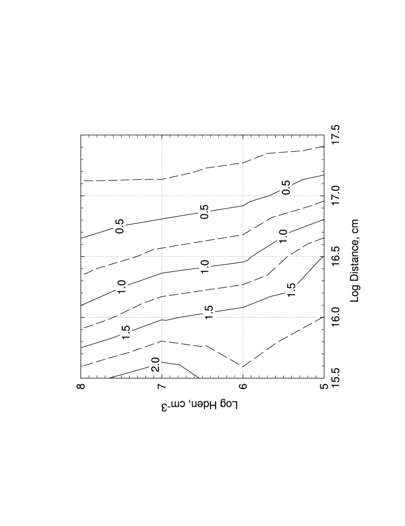
Figure 7: The $-$146 km s^-1 component: hydrogen density versus distance plot. The normalized ratio of the Fe II column densities for the a⁴F and a⁴D terms, R=(a⁴D/a⁴F)_theory/(a⁴D/a⁴F)_observation, was used to determine the optimal density/distance value. A value of unity for R indicates a match to the derived column density. At a distance of 10^16.1 to 10^16.4 cm, the hydrogen column density would be between 10⁷ to 10⁸ cm^-3.

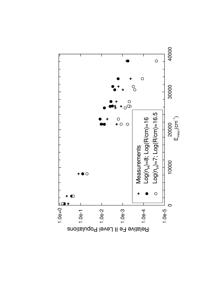
Figure 8: The observationally-derived and predicted Fe II relative level populations for the $-$146 km s^-1 component. The best fit lies between the two density values, possibly closer to n_H=10⁸ cm^-3. The theoretical and observed relative level populations roughly approximate a straight line for the three cases shown. The slope reflects the electron temperature, T_e, for each dataset. Most of the scatter is due to differing statistical weights for each level.

The most accurate measurements of the relative Fe II level populations (or column densities) are for the second (a ⁴F) and third (a ⁴D) configurations. We have constructed the theoretical level population ratio and scaled the other Fe II level populations derived from the curves-of-growth to this ratio. The Fe II relative energy level population ratio (R=n(a ⁴D)/n(a ⁴F)) is plotted in Figure 7 for a range of hydrogen densities from 10⁵ to 10⁸cm^-3 and a range of stellar distance between 10^15.5 and 10^16.5cm. The best models suggest the temperature range is from 5700 K to 7300 K, well bracketing the Fe II-inferred temperature of 6400 K (Figure 5). The predicted Fe II populations for the a⁴F and a⁴D terms are found to be in LTE. In Figure 8 the relative Fe II population levels are compared to the predicted level populations for n${}_{\mathrm{H}}=10^{7}$ and $10^{8}$cm^-3 at distances 10¹⁶ and 10^16.5 cm. From Figure 7, the normalized (unity) ratio indicates the stellar distance for the $-$146 km s^-1 to be 10^16.3 cm, or $\approx$1300 AU.

Independently, we repeated calculations for the $-$513 km s^-1 component. We measured only column densities for Ti II from the two lowest configurations as indicated above. Consequently, we cannot derive total hydrogen densities for this absorbing region. However, given the low deduced T_e and low ionization of this component, one must conclude that if it were at a distance comparable or less than the $-$146 km s^-1 component, it would necessarily have a higher density. Otherwise, the ionization and temperature would be much higher than the T_e = 760 K found. From a purely qualitative argument, we conclude the $-$513 km s^-1 component, unless it has exceptionally high densities, is at a distance much farther than 1300 AU.

For convenience, we adopt a n${}_{\mathrm{H}}\geq$10⁷cm^-3, similar to that found for the 146 km s^-1 component. Again, we assume the same stellar luminosity, but use the temperature derived from the Ti II energy populations, T_e=760 K. Our photoionization modeling then places the $-$513 km s^-1 component eight times more distant, or r$\approx$10,000 AU from the stellar source.

Based upon our modeling, we present the deduced physical conditions for the $-$146 km s^-1 and the $-$513 km s^-1 components in Table 5. Of course, these results are somewhat dependent upon the gaseous elemental depletions for Fe ($-$146 km s^-1) and the Ti ($-$513 km s^-1). We have also ignored possible shielding in these calculations. For example, if other components, lying between the central stellar source and the $-$146 km s^-1 and $-$513 km s^-1, produce significant attenuation of the $\eta\ Car$ radiation field, then this would reduce the implied distance for that component.

4 Interpretation

The geometry of the Homunculus, based upon STIS CCD long aperture spectra of nebular emission and absorption lines originating from the interior surface of the expanding debris, has been determined to be a bipolar lobed structure at an inclination angle of $\sim$41^o degrees with respect to the plane of the sky (Davidson et al. 2001). Spatial variations along the slit are resolved at the $0\,\farcs 1$  level, a projected scale of about 230 AU at the distance of $\eta\ Car$. The line-of-sight, centered on $\eta\ Car$, passes almost tangentially through the foreground lobe of the Homunculus, and likely intersects clumps of corresponding size. The Homunculus is a relatively thin shell. However, the analysis of Davidson et al (2001) used the emission of [Fe II] and [Ni II] lines to describe what appeared to be a relatively diffuse, but thin interior surface of the Homunculus. N. Smith (private communication) comments that the infrared spectroscopy of the Homunculus is consistent with a shell about one-tenth the thickness of the distance from $\eta\ Car$, and with a relatively diffuse interior skin and very thin outer skin.

The $-$513 km s^-1 component is likely part of the Homunculus in the line-of-sight. Based upon its relatively small b-value, it may be associated with the thin outer skin. Likewise, the detected components with velocities between $-$385 and $-$585 km s^-1 are evidence for clumps within the relatively thick wall of the Homunculus. Interior to the Homunculus is a large cavity, filled with a hot, very low density gas, too faint to be detected by current observations. Still interior is the Little Homunculus (Ishibashi et al. 2003) that is a thin, ionized shell with measured velocities in the vicinity of $-$146 km s^-1. Expansion velocities and proper motions of both the Homunculus and the Little Homunculus are consistent with ejection during the major outburst in the 1840’s and the lesser outburst in the 1890’s. The central region, immediately surrounding $\eta\ Car$, is thought to be a wind-blown cavity, with an extended skirt whose plane is perpendicular to the axis of the two lobes. In this picture, the two major velocity components seen in the STIS NUV spectra arise in the gas ejected during each of the two outbursts. The other velocity components, intermediate in velocity space, likely are components of the outer Homunculus, distributed in that one-tenth thickness, but projected along a long line of sight due to geometry. We note in passing that these multiple components are photoionized (or excited) by $\eta\ Car$, and that during the minimum, very significant changes occur. Data have been obtained during the 2003.5 minimum with the STIS, analysis on the temporal variability is ongoing.

The presence of dust and its effects on the excitation of these ejecta components appears to be surprisingly little. However, given the hot, low-density cavities bounded by the Little Homunculus and by the interior wall of the Homunculus, little dust intervenes between the star and the Little Homunculus, and in turn between the Little Homunculus and the outer Homunculus. The bulk of the dust is likely contained in the clumps of ejecta in line of sight. Hence we might expect to see some dust contribution in the thin wall of the Little Homunculus ($-$146 km s^-1 component) and considerably more dust contributions in the thicker wall of the Homunculus. Indeed dust is present in the Homunculus and is the scatterer for the stellar radiation seen reflected of the bipolar lobes. Smith et al (2003) demonstrated that the Balmer alpha (H$\alpha$) P-Cygni line profile changed across the 5.54-year cycle consistent with the terminal wind velocity increasing to about 1200 km s^-1 during the maximum and dropping to about 600 km s^-1 during the minimum. These changes in wind velocity are interpreted to originate from the high latitudes of the central source and that the dust in the relatively flat polar regions of the Homunculus has an optical depth of order unity, therefore causing a single scattering event between the star and the observer. Given the very lumpy appearance of the flat polar region and the relatively linear striations of the walls of the Homunculus, dust appears to be clumpy in distribution in the outer structure of the Homunculus. The simplest interpretation is that most of the dust in line of sight resides in the outer wall of the Homunculus and that some may lie in the interior thinner wall of the Little Homunculus. Certainly the presence of Fe II absorption lines in the Little Homunculus and Fe I absorption lines in the Homunculus indicates that much of the FUV radiation is stopped by the Little Homunculus. Some FUV radiation down to the Lyman limit does get through the wall as the STIS FUV and FUSE spectra show complex, but relatively continuous UV radiation to well below 1000 Å originating from a nearly point-like source. However no locally emitted Balmer line emission is detected from the Homunculus, but near-red [Fe II] and [Ni II] emission lines are present and were used by Davidson et al. (2001) to trace the geometrical structure of the Homunculus. The emission line velocities of the Little Homunculus and the Homunculus in the line of sight are in good agreement with the absorption velocities we see. Thus, the simplest interpretation of these absorption components are that they are associated with the expanding ejecta, not clumps within the much hotter wind within a few hundred AU of the star.

Many of the elements identified in these velocity components are refractory, with condensation temperatures below 1300 K. In a later paper we plan to address relative abundances, but initial inspection indicates that elemental depletion is low and not following a Spitzer-Routly law (Routly & Spitzer 1952). In particular the presence of V II and Ti II at $-$513 km s^-1 is remarkable. We speculate that the combination of low C and O abundances, the expanding ejecta and/or the modulated wind may inhibit normal grain formation in the $\eta\ Car$ system.

5 Conclusions

The UV STIS spectrum of $\eta\ Car$ reveals complex multiple, narrow absorption features for many neutral and singly-ionized species, spanning a velocity range from $-$146 km s^-1 to $-$585 km s^-1. Two narrow velocity components ($-$146 and $-$513 km s^-1) appear to originate from shells or clumps in the foreground lobe of the Homunculus. These clumps are heated by the very bright UV flux of $\eta\ Car$. The presence of ionic transitions up to energies of 40,000 cm^-1 is, in part, due to the high density in ejecta giving rise to the observed very strong circumstellar absorptions. The photoionization modeling for the $-$146 and the $-$513 km s^-1 components suggest that the corresponding absorptions arise at large distances from the central stellar source. We conclude that the absorption is formed in dense gas located at different positions within the bipolar structure of the Homunculus. The $-$146 km s^-1 component is formed at a distance of $\sim$1300 AU, which leads to a spectrum consisting mainly of lines from singly-ionized iron-group ions. The $-$146 km s^-1 component is likely formed in the wall of the Little Homunculus (Ishibashi et al. 2003). Although the conclusion is less firm, the cooler $-$513 km s^-1 component, seen in the lines of neutral and singly ionized elements, appears to be formed at a much larger distance from the star ($\sim$10,000AU). This component is likely formed in the wall of the Homunculus. Further analysis of the STIS dataset for $\eta\ Car$, including changes that occur during the 2003.5 minimum will be presented in subsequent papers.

Table 1: Fe II lines used in the $-$146 km s^-1 component analysis

Lower Level	$\lambda_{\mathrm{lab}}$	Vel.	Jlow	Elow	Wλ	log ($gf$)	Ref.
	(Å)	(km s-1)		(cm-1)	(Å)
(5D)4s a6D
	2586.650	$-$143.8	4.5	0.000	0.224	$-$0.19	FMW
	2600.173	$-$145.9	4.5	0.000	0.264	0.35	FMW
	2599.147	$-$145.2	3.5	384.790	0.165	$-$0.10	FMW
	2399.973	$-$144.8	2.5	667.683	0.184	$-$0.15	FMW
	2407.394	$-$144.9	1.5	862.613	0.176	$-$0.25	FMW
	2614.605	$-$142.9	1.5	862.613	0.180	$-$0.39	FMW
	2621.191	$-$146.0	1.5	862.613	0.050	$-$1.83	FMW
	2414.045	$-$145.2	0.5	977.053	0.165	$-$0.43	FMW
	2622.452	$-$146.1	0.5	977.053	0.119	$-$1.00	FMW
d7 a4F
	2451.842	$-$146.4	4.5	1872.567	0.031	$-$2.07	K88
	2484.951	$-$146.5	4.5	1872.567	0.047	$-$1.98	K88
	2392.206	$-$146.7	3.5	2430.097	0.056	$-$1.64	FMW
	2505.969	$-$147.0	3.5	2430.097	0.022	$-$2.22	K88
	2512.125	$-$146.6	3.5	2430.097	0.018	$-$2.53	K88
(5D)4s a4D
	2563.304	$-$144.7	3.5	7955.299	0.156	$-$0.05	FMW
	2693.633	$-$146.5	3.5	7955.299	0.026	$-$2.09	FMW
	2715.218	$-$146.2	3.5	7955.299	0.256	$-$0.44	FMW
	2740.358	$-$145.8	3.5	7955.299	0.203	0.24	FMW
	2756.551	$-$144.8	3.5	7955.299	0.224	0.38	FMW
	2881.601	$-$145.5	3.5	7955.299	0.041	$-$1.66	FMW
	2927.441	$-$146.9	3.5	7955.299	0.085	$-$1.23	FMW
	2564.245	$-$146.0	2.5	8391.938	0.151	$-$0.29	FMW
	2869.716	$-$147.0	2.5	8391.938	0.012	$-$2.29	FMW
	2940.367	$-$146.7	2.5	8391.938	0.008	$-$2.75	FMW
	2567.683	$-$145.3	1.5	8680.454	0.098	$-$0.65	FMW
	2731.542	$-$145.7	1.5	8680.454	0.082	$-$0.95	FMW
	2769.753	$-$146.4	1.5	8680.454	0.047	$-$1.51	FMW
	2762.629	$-$147.1	0.5	8846.768	0.068	$-$1.28	FMW

References. — (FMW) $-$ Fuhr J. R., Martin G. A, and Wiese W. L. 1988, J. Phys. Chem. Ref. Data 17, Suppl. 4, (K88) $-$ Kurucz R. L. 1988, In: McNally M. (ed.) Trans. IAU, XXB, Kluver, Dordrecht, p. 168

Table 2: Ti II Lines used in $-$513 km s^-1 Component Analysis

Lower Level	$\lambda_{\mathrm{lab}}$	Vel.	Jlow	Elow	Wλ	log ($gf$)
	(Å)	(km s-1)		(cm-1)	(Å)
(3F)4s a4F
	3058.282	$-$513.1	1.5	0.00	0.016	$-$1.78
	3067.238	$-$513.5	1.5	0.00	0.053	$-$0.71
	3073.863	$-$512.5	1.5	0.00	0.070	$-$0.32
	3122.515	$-$514.4	1.5	0.00	0.006	$-$2.36
	3148.948	$-$513.0	1.5	0.00	0.043	$-$1.22
	3060.634	$-$513.9	2.5	94.10	0.012	$-$1.57
	3067.109	$-$513.3	2.5	94.10	0.052	$-$0.59
	3076.117	$-$512.5	2.5	94.10	0.080	$-$0.12
	3131.706	$-$513.0	2.5	94.10	0.026	$-$1.19
	3158.307	$-$513.7	2.5	94.10	0.008	$-$2.17
	3073.000	$-$512.9	3.5	225.73	0.046	$-$0.62
	3079.539	$-$512.6	3.5	225.73	0.081	0.06
	3144.665	$-$512.4	3.5	225.73	0.019	$-$1.30
	3088.922	$-$512.1	4.5	393.44	0.085	0.23
d3 b4F
	2536.632	$-$512.1	1.5	908.02	0.009	$-$1.03
	3155.106	$-$512.2	1.5	908.02	0.016	$-$1.15
	3162.117	$-$512.1	1.5	908.02	0.023	$-$0.69
	2535.381	$-$512.9	2.5	983.89	0.012	$-$0.94
	3153.163	$-$510.7	2.5	983.89	0.012	$-$1.06
	3162.684	$-$512.0	2.5	983.89	0.032	$-$0.55
	2532.013	$-$512.7	3.5	1087.32	0.012	$-$0.67
	3156.582	$-$510.9	3.5	1087.32	0.008	$-$1.17
	3163.481	$-$512.1	3.5	1087.32	0.033	$-$0.38
	2526.362	$-$512.8	4.5	1215.84	0.014	$-$0.51

Table 3: Column densities from the $-$146 km s^-1 Fe II curve-of-growth analysis.

	Conf.	Emean(cm-1)	ni(1013 cm-2)
	4s$\!{}^{\mathrm{\,}}$ a 6D	416	169.9
	3d$\!{}^{\mathrm{7}}$ a 4F	2417	200.0
	4s$\!{}^{\mathrm{}}$ a 4D	8321	54.56
	a 4P	18007	59
	4s$\!{}^{\mathrm{}}$ b 4P	21421	0.83
	4s$\!{}^{\mathrm{}}$ a 4H	21459	3.85
	4s$\!{}^{\mathrm{}}$ b 4F	22808	2.34
	4s$\!{}^{\mathrm{}}$ a 4G	25761	0.95
	4s$\!{}^{\mathrm{}}$ b 2P	26169	0.51
	4s$\!{}^{\mathrm{}}$ b 2H	26253	0.99
	4s$\!{}^{\mathrm{}}$ a 2F	27445	0.86
	4s$\!{}^{\mathrm{}}$ b 2G	30556	0.42
	4s$\!{}^{\mathrm{}}$ b 4D	31421	0.68
	4s$\!{}^{\mathrm{}}$ a 2I	32892	–
	4s$\!{}^{\mathrm{}}$ c 2G	33482	0.18
	4s$\!{}^{\mathrm{}}$ c 2D	38184	0.28
N =$\sum_{i}{\mathrm{n}_{i}}$			495

Table 4: Column densities from the $-$513 km s^-1 Ti II curve-of-growth analysis.

	Conf.	Emean(cm-1)	ni (1013 cm-2)
	4s$\!{}^{\mathrm{\,}}$ a 4F	225	16
	3d$\!{}^{\mathrm{3}}$ b 4F	1085	3
N = $\sum_{i}{\mathrm{n}_{i}}$			19

Table 5: Physical parameters for the $-$146 and $-$513 km s^-1components

	$-$146 km s-1	$-$513 km s-1
b-value	5.5 km s-1	2.1 km s-1
Derived Te:	6400 K	760 K
Ionization	Singly Ionized Species	Neutral &
		Singly Ionized Species
Hydrogen density, ne:	$\geq$107cm-3	$\geq$107cm-3
Distance from star	$\sim$1300 AU	$\sim$10,000 AU

Figure 1: Spectral region of Mg I $\lambda$2853 for $\eta\ Car$, HDE 303308 and CPD $-$59° 2603, all members of the Carinae association. Strong intervening IS absorption velocities are $+$100 to $-$50 km s^-1 (Walborn et al. 2002). Unique to the $\eta\ Car$ spectrum are the prominent absorption line at $-$146 km s^-1 and the multiple, narrow absorption lines between $-$385 and $-$585 km s^-1. The $\eta\ Car$ spectrum includes a slowly varying P-Cygni profile in addition to a series of narrower absorption components between $-$146 and $-$585 km s^-1.

Figure 2: Comparison of circumstellar absorption line profiles for selected observed transitions. These normalized spectral profiles are for transitions from a range of lower levels for several neutral and singly-ionized elements. The $-$513 km s^-1 component is the narrowest, yet absorption lines originate from levels up to 7400 cm^-1above ground. Note that many Fe I, V II and Ti II lines are unique to the $-$513 km s^-1 component. The $-$146 km s^-1 component is from singly-ionized, iron-peak and other elements, includes transitions from even higher energy levels and is characteristically broader than the lines of the $-$513 km s^-1 component. The complicated velocity structure between $-$380 to $-$513 km s^-1 is noticeable for the two Fe II lines. The two Fe II lines also have a very broad wind component, starting from $-$250 km s^-1 and extending into the portion of the spectrum of the narrow line components. Spatial resolution of these structures demonstrate that the wind feature is very distinct from the narrow velocity components.

Figure 3: The $-$146 km s^-1 Component curves-of-growth plots for the lowest three terms of Fe II. Measured lines were selected to minimize blending with other velocity components, to be measurable against the relatively complex stellar spectrum. The relatively large uncertainty bars are due to ability to determine the continuum level of $\eta\ Car$, and not photon statistics. Note that all three curves-of-growth are consistent with a b-value of 5.5 km s^-1.

Figure 4: The $-$513 km s^-1 Component curves-of-growth plots for the lowest two terms of Ti II. The $-$513 km s^-1 component is much narrower in width and is seen in lines originating from significantly lower energy levels that seen either in the P-Cygni wind of $\eta\ Car$ or in the multiple absorption components similar in excitation to the $-$146 km s^-1 component. No lines originating from higher energy levels were found. Thus the populations of these two terms are found to be the major contributors to the total amount of Ti II.

Figure 5: Fe II population for each energy level of the $-$146 km s^-1 component. The linear slope corresponds to 6370 K. Note that the population for each energy level is normalized by the statistical weight.

Figure 6: Ti II population for each energy level of the $-$513 km s^-1 component. The linear slope corresponds to 760 K.

References

- Cardelli (1994) Cardelli, J., 1994, Science, 265, 209
- Davidson & Humphreys (1999) Davidson, K. & Humphreys, R., 1999, ARA&A, 35, 1
- Davidson et al. (2001) Davidson, K. et al. 2001, AJ, 121, 1569
- Heger & Woosley (2003) Heger, A., & Woosley, S. 2003, ApJ, 567, 532
- Hillier et al. 2001 (2001) Hillier, D.J., Davidson, K., Ishibashi, K. & Gull, T. 2001, ApJ, 553, 837
- Ishibashi et al. (2003) Ishibashi, K. et al. 2003, AJ, 125, 3222
- Lindler (1999) Lindler, D., 1999, CALSTIS Reference Guide http://hire.gsfc.nasa.gov/stis/software
- Kurucz (1979) Kurucz, R., 1979, ApJS,40,1
- Kurucz (1988) Kurucz, R., 1988, In: McNally M. (ed.) Trans. IAU, XXB, Kluver, Dordrecht, 168
- Martin (1988) Martin, G. A., Fuhr, J.R. & Wiese, W.L., 1988 J. P:hys. Chem. Ref. Data 17 Suppl. 3
- Meaburn (1999) Meaburn, J., 1999, ASPCP, 179, 89
- Pickering, Thorne & Perez, (2001) Pickering, J., Thorne, A. & Perez, R. 2001, ApJS, 132, 403
- Pickering, Thorne & Perez, (2002) Pickering, J., Thorne, A. & Perez, R. 2002, ApJS, 138, 247
- Routly & Spitzer (1952) Routly, P., & Spitzer, L., 1952, ApJ, 115, 227
- Snow, Weiler & Oegerle (1979) Snow, T., Weiler, E. & Oegerle, W., 1979, ApJ, 234,506
- Smith et al (2003) Smith, N., et al., 2003, AJ, 586, 432
- Smith et al (2004) Smith, N., et al., 2004, ApJ, 605, 405
- Verner et al. (1999) Verner, E., Verner, D., Korista, K., Ferguson, J. Hamann, F., & Ferland, G. , 1999, ApJS, 120, 101
- Verner et al. (2002) Verner, E., Gull, T.R., Bruhweiler, F., Johansson, S., Ishibashi, K., & Davidson, K., 2002, ApJ, 581, 1154
- Verner, Bruhweiler, & Gull (2004) Verner, E., Bruhweiler, F., & Gull, T., 2004, ApJ, submitted
- Viotti, (1976) Viotti, R., 1976, ApJ, 204, 293
- Walborn et al. (2002) Walborn, N., Danks, A., Vieira, G., & Landsman, W., 2002, ApJS, 140, 407
- Wiese & Fuhr (1988) Weise, W.L. & Fuhr, J.R., 1988, J. Phys. Chem. Ref. Data 4, 263
- Welty et al. (1992) Welty, D., Thorburn, J., Hobbs, L., & York, D., 1992, PASP,104, 737