Subarcsecond mid-infrared and radio observations of the W3 IRS5 protocluster

Observations at mid-infrared (4.8–17.65 $\mu$m) and radio (0.7–1.3 cm) wavelengths are used to constrain the structure of the high-mass star-forming region W3 IRS5 on 0$.\!\!^{\prime\prime}$1 (200 AU) scales. Two bright mid-infrared sources are detected, as well as diffuse emission. The bright sources have associated compact radio emission and probably are young high-mass stars. The measured sizes and estimated temperatures indicate that these sources together can supply the observed far-infrared luminosity. However, an optically thick radio source with a possible mid-infrared counterpart may also contribute significant luminosity; if so, it must be extremely deeply embedded. The infrared colour temperatures of 350–390 K and low radio brightness suggest gravitational confinement of the H II regions and ongoing accretion at a rate of a few 10^-8 M_⊙ yr^-1 or more. Variations in the accretion rate would explain the observed radio variability. The low estimated foreground extinction suggests the existence of a cavity around the central stars, perhaps blown by stellar winds. At least three radio sources without mid-infrared counterparts appear to show proper motions of $\sim$100 km s^-1, and may be deeply embedded young runaway OB stars, but more likely are clumps in the ambient material which are shock-ionized by the OB star winds.

1 Introduction

Figure 1: Images of W3 IRS5 at 43 GHz (left) and 22 GHz (right). Contours start at 4$\sigma$ and increase by 2$\sigma$, where $\sigma$=0.16 mJy/beam at 43 GHz and 0.15 mJy/beam at 22 GHz.

Stars of masses $>$8 M_⊙ spend a significant fraction of their lifetimes, $>$10%, embedded in their natal molecular clouds. Single-dish (sub)millimeter observations have clarified the structure of high-mass protostellar envelopes on $\sim$10⁴–10⁵ AU scales (see Hatchell & van der Tak 2003 and references therein). However, the distribution and kinematics of material on ${{}_{<}\atop{{}^{\sim}}}$1000 AU scales is poorly known, due to the large (${{}_{>}\atop{{}^{\sim}}}$1 kpc) distances involved, and the lack of tracers at optical and near-infrared wavelengths. These scales are of great interest to decide between formation mechanisms for high-mass stars, and to clarify the relation with clustered star formation (Churchwell, 2002). Does the distribution of stellar masses in a star-forming region depend on the stellar density? Also, the origin of the observed outflows and their interaction with the environment on ${{}_{<}\atop{{}^{\sim}}}$1000 AU scales remain unclear. Subarcsecond resolution observations are necessary to shed light on these and other questions, which, at (sub)millimeter wavelengths, are just coming within reach (Beuther et al., 2004). However, these resolutions can already be achieved in both the infrared and radio wavebands, where extinction is much smaller than in the optical.

In the infrared, high-resolution techniques are most advanced at near-infrared wavelengths. Such observations probe less embedded, more evolved phases, where a significant part of the surroundings is already ionized. Important progress has been made with the identification of the ionizing stars of several ultracompact H II regions (e.g., Watson & Hanson 1997, Feldt et al. 2003). In the case of intermediate-mass stars, the imaging of the hot inner regions of disks is presently generating a lot of interest (Danchi et al. 2001; Tuthill et al. 2001). In addition, a few more embeddded objects have been probed (Weigelt et al. 2002; Preibisch et al. 2002), although in the general case long baseline interferometers will be needed to tackle most targets given the characteristic size scales involved (Monnier & Millan-Gabet, 2002). At mid-infrared wavelengths, pioneering work has been done by Walsh et al. (2001), but subarcsecond resolution has only recently been achieved (Tuthill et al. 2002; De Buizer et al. 2002; Greenhill et al. 2004).

In the cm-wave region, most subarcsecond-resolution studies have concentrated on H₂O masers, which are bright enough for Very Long Baseline Interferometry (VLBI) observations. The excitation requirements of the masers are such that the emission usually traces shocks associated with infalling or outflowing motions. The VLBI data indicate that the maser emission traces moving gas parcels, rather than shock waves propagating through an H₂O–rich cloud. In the case of outflow motions, both bipolar and spherical flows are seen, which may represent different stages of evolution (Torrelles et al., 2003). In some cases, H₂O masers in star-forming regions may arise in accretion shocks in infalling gas (Menten & van der Tak, 2004).

Continuum emission at centimeter wavelengths arises in ionized gas. In stellar winds and outflows, the gas can be collisionally ionized, and VLBI data indicate a mixture of bipolar and equatorial outflows (Hoare, 2002). Close to hot stars, small regions of photo-ionized gas are observed as ‘hypercompact’ H II regions, which represent a very early stage of high-mass star formation (Garay & Lizano, 1999).

At a distance of 1.83$\pm$0.14 kpc (Imai et al., 2000), W3 IRS5 is the nearest region of high-mass ($L$=1.2$\times$10⁵ L_⊙: Ladd et al. 1993) star formation after Orion. The bright mid-infrared source has been resolved into a double (Howell et al. 1981; Neugebauer et al. 1982). Single-dish submillimeter mapping indicate an envelope mass of 262 M_⊙ within a radius of 60,000 AU, with an $r^{-1.5}$ density distribution (van der Tak et al., 2000). Near-infrared imaging shows a dense cluster ($\sim$3000 pc^-3: Megeath et al. 1996), mostly composed of low-mass pre-main-sequence stars with ages 0.3–1 Myr (Ojha et al., 2004). Radio continuum observations show a cluster of at least six ‘hypercompact’ H II regions labeled A…F (Claussen et al. 1994; Tieftrunk et al. 1997), at least one of which exhibits proper motions (Wilson et al., 2003). Water maser mapping reveals $\sim$100 spots, grouped in two flows: one roughly spherical and centered close to continuum source A, and the other more collimated and centered close to source D (Claussen et al. 1994; Imai et al. 2000). Mid-infrared spectroscopy shows CO absorption features blueshifted by 4..46 km s^-1 relative to the systemic velocity (Mitchell et al., 1991), which must arise in an outflow. In millimeter-wave CO emission, blue- and redshifted outflow lobes are detected out to $\approx$23 km s^-1 from the systemic velocity (Claussen et al., 1984), indicating that the highest-velocity gas is very compact. Finally, Chandra observations by Hofner et al. (2002) indicate an X-ray luminosity of W3 IRS5 of $L_{X}$=9$\times$10²⁹ erg s^-1 (for $d$=1.83 kpc), consistent with the typical values for T Tauri stars.

This paper presents new cm-wave and mid-infrared images of W3 IRS5 at sub-arcsecond resolution. The goals are to clarify the nature of the radio continuum sources and their relation with the infrared double, to find which ones are self-luminous, and which ones power the region.

2 Observations

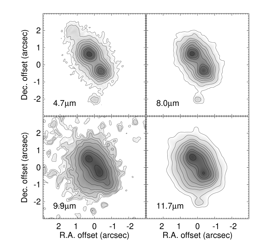
Figure 2: Mid-infrared long-exposure images of W3 IRS5. Contours are at 0.5, 1, 2, 3, 5, 10, 20, 30 and 70% of the peak intensity.

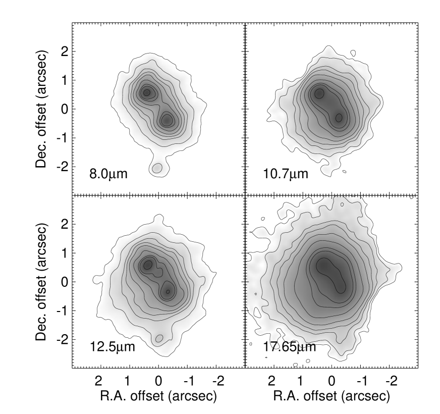
Figure 3: Mid-infrared ‘speckle’ images of W3 IRS5. Contours are at 0.5, 1, 2, 3, 5, 10, 20, 30 and 70% of the peak intensity.

2.1 Radio Observations

Radio observations of W3 IRS5 were carried out with the NRAO Very Large Array (VLA) on 1996 October 24, when the VLA was in its $A$-configuration. At this time, thirteen VLA antennas were equipped with 43 GHz receivers; the other fourteen observed at 22 GHz (respectively known as Q- and K-band in radio astronomy). Zenith opacity was 0.089 at 22.5 GHz and 0.071 at 43.3 GHz. Elevation-dependent antenna gains were interpolated from values measured by the VLA staff. The phase calibrator, 0228+673, was observed every 10 minutes at 43 GHz and every 15 minutes at 22 GHz (the ‘fast switching’ procedure was not implemented at the time). Pointing was checked at 8.4 GHz on the same source every 70 minutes at 43 GHz and every 5 hours at 22 GHz. On-source integration time is 438 min at 22 GHz and 400 min at 43 GHz. The data were edited, calibrated, and imaged with NRAO’s Astronomical Image Processing System (AIPS). Absolute calibration was obtained from observations of 3C 286 using flux densities interpolated from the values given by Ott et al. (1994). For 0228+673, we obtain a flux density of 1.83 Jy at 22 GHz and 1.55 Jy at 43 GHz.

Figure 1 shows the 22 and 43 GHz maps, which have rms noise levels of 0.15 and 0.16 mJy beam^-1. These maps were obtained from the $uv$ data by a Fourier transform with uniform weighting, and deconvolved with the Clean algorithm. Restoring beam major and minor axes and position angles are 44$\times$37 mas at position angle –68^∘ at 43 GHz and 89$\times$88 mas, PA –53^∘ at 22 GHz.

2.2 Infrared Observations

Data were obtained in August 2002 with the Long Wavelength Spectrometer (LWS) camera on the Keck I telescope. Two different observing methodologies were employed. The first set of observations utilized a standard chop-nod pattern, with frames coadded to build up longer exposure times. Observations of W3 IRS5 (with the calibrator $\xi$ Cyg) taken in this mode emphasized the recovery of faint structure. The second mode had a fast readout in addition to the chop-nod, so that large volumes of rapid exposure data were collected in a fashion analogous to a mid-IR ‘speckle’ experiment, with the hope to recover fine structure in the images. Again, these objects were paired with similar data taken on a point source calibrator, this time $\alpha$ Ceti. No point-source calibrator files were taken for 9.9 $\mu$m or 12.5 $\mu$m observations. These two modes are denoted ‘L’ and ‘S’ for ‘long’ and ‘speckle’ exposure hereafter.

Data have been analyzed with an iterative matched filter version of the shift-and-add algorithm. This algorithm attempts to match the shifts in the current iteration to maximise the correlation with the output of the previous iteration. Significant gains in image resolution were demonstrated over straight coadding, while a simple shift-and-add strategy was foiled in this case by the presence of two nearly equal peaks.

Figures 2 and 3 present the resultant images, except the 17.65 $\mu$m long-exposure image which is very similar to the speckle image at that wavelength. Note that an artifact due to an unwanted reflection from an optical surface affects the 4.7 $\mu$m image, giving a spurious feature to the North-East which is not seen at any other wavelength. This ‘ghost’ was also present in point-source calibrator data in this filter. The 9.9 $\mu$m and (to a lesser extent) the 10.7 $\mu$m data have degraded signal-to-noise due to the much lower flux levels. There were, unfortunately, additional experimental difficulties which were not easy to account for. The observations were taken under conditions of variable cirrus, increasing the errors in photometry. Compounding this was an intermittent mechanical fault with the camera mechanism which resulted in partial occultation of the pupil, affecting both the throughput and the point-spread function (PSF). Although this had little effect on the maps presented here, it did preclude our original intent of fully deconvolving the images using the PSF from the reference star observations.

3 Results

Table 1: Radio emission from W3 IRS5. Numbers in brackets are uncertainties in units of the last decimal.

Source	$\alpha$	$\delta$	Peak $I_{\nu}$	Total $S_{\nu}$	Major axis	Minor axis	PA
	(J2000)	(J2000)	mJy/beam	mJy	mas	mas	deg
Q1	02 25 40.660407(635)	62 05 51.82215(404)	0.691(162)	0.78(31)	45(10)	41(10)	93(90)
Q2	02 25 40.676344(379)	62 05 52.04937(261)	1.285(158)	1.92(36)	59(7)	41(5)	47(13)
Q3	02 25 40.681511(211)	62 05 51.53000(198)	2.102(155)	3.89(42)	63(5)	47(3)	7(10)
Q4	02 25 40.728475(704)	62 05 49.85180(702)	0.666(154)	1.43(46)	75(17)	46(11)	21(18)
Q5	02 25 40.783441(212)	62 05 52.46552(141)	1.996(163)	2.19(30)	43(4)	41(3)	88(57)
K1	02 25 40.143241(1234)	62 05 52.28144(1080)	0.745(142)	0.85(27)	139(27)	99(19)	25(22)
K2	02 25 40.661233(1029)	62 05 51.86622(1174)	0.847(140)	1.08(29)	175(29)	88(15)	160(9)
K3	02 25 40.675758(1135)	62 05 52.04087(690)	0.857(142)	0.76(23)	121(20)	88(15)	59(21)
K4	02 25 40.682172(526)	62 05 51.54376(441)	1.938(139)	2.76(31)	152(11)	113(8)	154(10)
K5	02 25 40.712459(785)	62 05 52.44786(569)	1.163(142)	1.12(24)	110(13)	106(13)	168(138)
K6	02 25 40.733047(1601)	62 05 49.84977(1214)	0.797(134)	1.76(41)	174(29)	154(26)	25(56)
K7	02 25 40.782747(737)	62 05 52.46103(637)	1.313(140)	1.63(28)	150(16)	100(11)	29(10)
K8	02 25 40.861211(888)	62 05 53.46070(717)	1.307(135)	2.44(37)	169(17)	135(14)	25(19)

3.1 Radio Positions

Table 1 lists the sources detected above 5$\sigma$ using the multiple-peak-finding AIPS task SAD after trying various weighting schemes. For the $Q$–band data, the table uses the image obtained with uniform weighting, which has better positional accuracy, while for the $K$–band data, tabulated results use an image obtained with natural weighting, where more sources are detected (rms = 142 $\mu$Jy). Sources Q1 and Q4 are 4$\sigma$ detections and were not found by SAD, but their detection is secure because they have $K$–band counterparts. The flux densities in the table are corrected for primary beam response. Positional uncertainties are statistical errors and apply to the relative positions of these radio sources.

Columns 6–8 of Table 1 gives the source sizes. Since only sources Q3, K6 and K8 appear marginally resolved, the sizes have not been deconvolved. The sizes would be lower limits if extended emission is resolved out by the interferometer (Kurtz et al. 1999; Kim & Koo 2001). In the particular case of W 3 IRS5, however, multi-configuration observations rule out extended emission down to very low limits (Tieftrunk et al., 1997). Therefore, the radio sources of W3 IRS5 belong to the class of ‘hypercompact’ H II regions (Kurtz & Franco, 2002).

Comparing the positions in Table 1 with those from 1989 (Claussen et al. 1994; Tieftrunk et al. 1997) leads to the following identifications: Q1 = K2, Q2 = K3 = A, Q3 = K4 = B, Q4 = K6, Q5 = K7 = MD1, K5 = C, K8 = F. Source K1 is several arc seconds away and probably unrelated. Sources Q1=K2 and Q4=K6 were not seen before and appear to be new. On the other hand, sources E and G seem to have disappeared since 1989, the epoch when the Tieftrunk et al data were taken. Most strikingly, source D2 has disappeared, which is remarkable since it was the strongest source in 1989. Perhaps D1 and D2 were not separate sources, but merely substructure within one source, which we refer to as D hereafter.

Our sources with counterparts in the old data do not exactly lie on the positions reported by Claussen et al. (1994) and Tieftrunk et al. (1997), but rather at 80–140 mas shifts. The shifts are 2–3 beam sizes and $>$10 times the formal error on relative positions. The position angles of the shifts vary between 20^∘ and 60^∘, which argues against instrumental effects such as pointing errors or changes in calibrator positions, which would shift all sources in the same direction. The data thus seem to confirm the existence of proper motions reported by Wilson et al. (2003). At a distance of 1.83 kpc, a motion of 100 mas in 7.48 yr corresponds to a transverse velocity of 116 km s^-1. The space velocity may be a factor $\sqrt{2}$ higher, or 164 km s^-1. These values are much larger than the motions of the H₂O masers of $\sim$20 km s^-1 (Imai et al., 2000) and of the CO emission and absorption (§ 1).

3.2 Infrared Positions

Table 2: Quantitative analysis of the infrared imaging: flux densities and relative positions. The table columns are arranged as follows: (1) observing $\lambda/\Delta\lambda$; (2) speckle ‘S’ or long ‘L’ exposure; (3) FWHM of point-source reference star; (4,6,10) flux of MIR 1–3; (5,7,11) FWHM of MIR 1–3; (8,12) separation of sources MIR1-2 and MIR1-3; (9,13) position angle of sources MIR1-2 and MIR1-3; (14) total flux detected.

Filter	Mode	PSF star	MIR1		MIR2		MIR1-MIR2		MIR3		MIR1-MIR3		Total
$\lambda/\Delta\lambda$	L/S	FWHM	flux	FWHM	flux	FWHM	Sep	PA	flux	FWHM	Sep	PA	Flux
($\mu$m)		(mas)	(Jy)	(mas)	(Jy)	(mas)	(mas)	(deg)	(Jy)	(mas)	(mas)	(deg)	(Jy)
4.8/0.6	L	507	44	453	23	471	1217	215	0.6	480	2730	186	80
8.0/0.7	L	384	140	432	108	480	1198	215	2.0	436	2741	187	301
8.0/0.7	S	258	152	310	123	367	1214	217	1.8	304	2663	188	328
9.9/0.8	L	-	4	576	4	568	1013	215	$<0.5$	-	-	-	11
10.7/1.4	S	291	13	460	12	552	1078	219	$<1.2$	-	-	-	32
11.7/1.0	L	364	60	519	50	607	1097	216	0.7	255	2739	187	142
12.5/0.9	S	-	60	467	50	587	1145	218	1.1	329	2632	188	146
17.65/0.9	L	451	98	716	92	636	1049	217	$<10.7$	-	-	-	318
17.65/0.9	S	452	107	646	93	615	1102	219	$<10.3$	-	-	-	323

The infrared images (Figs. 2 and 3) show three compact sources, surrounded by diffuse emission which becomes more pronounced toward longer wavelengths. We begin a quantitative analysis of these images by fitting simple profiles to the data, and by measuring flux densities in different regions. The results are given in Table 2, which gives the fluxes, relative positions and full-width at half-maximum (FWHM) of the various components. In addition, the FWHM of the point-source reference stars are given, which gives an estimate of the resultant system PSF. Examination of these data shows that the system appears truly diffraction-limited in either mode (‘L’ or ‘S’) at 17.65 $\mu$m. At shorter wavelengths (8.0–12.5 $\mu$m), the ‘S’ mode delivers a significantly smaller FWHM than ‘L’ (8.0 $\mu$m gives a direct comparison) which approaches the formal diffraction limit. The dramatic increase in size at 4.8 $\mu$m implies some optical problem beyond the normal effects of diffraction and seeing, such as optical aberration or defocus.

In the absence of a wide-field image with standard stars, our only astrometric information comes from the relative positions of the components. We refer to the northernmost bright component as MIR1, with MIR2 being of nearly equal brightness to the south, and MIR3 the much fainter southernmost peak. Table 2 lists the separation and the position angle of MIR2 & MIR3 relative to MIR1 for all observations, obtained through Gaussian fits to the emission.

The mean separation of MIR1 & MIR2 is 1124$\pm$74 mas at a position angle of 36.8$\pm$1.7 degrees. These values are consistent with those from earlier mid-infrared work (Howell et al. 1981; Neugebauer et al. 1982), but our data are the first to image the mid-infrared double directly.

We compare this relative position with those of pairs of radio sources. The best match is for pair Q3–Q5, whose separation of 1210 mas at a position angle of 37$.\!\!^{\circ}$4 is in good agreement with the infrared peaks. The only other radio pair with similar relative positions is K7–K8, which has a separation of 1141 mas, but at a position angle of 28$.\!\!^{\circ}$9, inconsistent with the infrared result. On this basis, we identify the bright mid-infrared sources with radio sources Q5=K7=MIR1 and Q3=K4=MIR2. The position of source MIR3, with 1–2% of the flux density of the main sources, then coincides with radio source Q4=K6, confirming our identification. There is a cluster of H₂O maser spots close to this object, at $\Delta$($\alpha$)$\approx$250 and $\Delta$($\delta$)$\approx$2000 mas (Imai et al., 2000). Table 3 summarizes our source identifications.

The images in Figures 2 and 3 show the only region of flux detected within the 10$.\!\!^{\prime\prime}$24 field of view of LWS, with one exception. In a few frames (which happened to be offset from center) a faint diffuse component was seen at the extreme edge of the field, 7$.\!\!^{\prime\prime}$3 from MIR1 at a position angle of 160^∘. Using the radio identifications of MIR1 and MIR2 as astrometric reference, this source, which we call MIR4, lies at position $\alpha$ = 02^h 25^m 41$.\!\!^{\mathrm{s}}$1388, $\delta$ = 62^∘ 05^′ 45$.\!\!^{\prime\prime}$604 (J2000), where no radio emission is detected. The extended nature and location at the edge of the field of view preclude measurement of its mid-infrared flux density.

Table 3: Radio and infrared identifications.

MIR	Q	K	1989
1	5	7	D
2	3	4	B
3	4	6	–
–	1	2	–
–	2	3	A
–	–	5	C
–	–	8	F
–	–	–	E
–	–	–	G
–	–	1	–

3.3 Radio Brightness

The flux densities of 22 GHz sources K3, K4, K5, K7 and K8 are significantly different from the values by Tieftrunk et al. (1997), probably due to variability. Instrumental effects, such as calibration problems, atmospheric decorrelation, or difference in beam size, would affect all sources in the same way. Instead, several components seem to undergo gradual increases or decreases in 22 GHz brightness over the available 13-year period (Figure 4).

The total flux densities in Table 1 indicate a spectral index $\gamma$, defined through

$$S_{\nu}\propto\nu^{\gamma}$$

of $\gamma$=1.42$\pm$0.77 for source Q2, $\gamma$=0.52$\pm$0.33 for source Q3, and $\gamma$=0.45$\pm$0.48 for source Q5. Values derived from the peak brightness are 0.62$\pm$0.44, 0.12$\pm$0.22 and 0.64$\pm$0.29. These values are consistent with thermal emission, and are not affected by variability as the data were taken simultaneously. For the weak 43 GHz sources Q1 and Q4, we find $\gamma$=–0.3$\pm$0.6, i.e., flat or slightly nonthermal spectra. Sources K1, K5 and K8, which are not detected at 43 GHz, have $\gamma$=–1$\pm$1 and may be of nonthermal nature. The spectral indices found here are consistent with those by Wilson et al. (2003), which are also based on simultaneous measurements, except for source K8=F which was detected at 43 GHz in 2002 but not in 1996.

In the case of Bremsstrahlung from an ionized region with a power law distribution of the electron density with radius,

$$n_{e}\propto r^{-q}$$

the spectral index is

$$\gamma=(2q-3.1)/(q-0.5)$$

(Olnon, 1975). Hence the spectral index of $\gamma\approx 0.5$ measured for Q3 and Q5 corresponds to $q\approx 1.9$, close to the value of $2$ for an ionized wind. Observations of broad H I radio recombination lines (Tieftrunk et al. 1997; Sewilo et al. 2004) support this interpretation, although higher angular resolution is needed to relate the line emission with the continuum sources. In any case, our measurements are not sensitive enough to rule out a flat radio spectrum for these sources, which would indicate optically thin emission. The objects could then be externally ionized, consistent with the absence of mid-infrared emission.

The value $\gamma\approx 1.5$ measured for Q2 could arise in an H II region with a constant density at the center and a steep ($q\approx 4.7$) outer fall-off. It is not clear which mechanism would create such a density distribution, especially since the sound speed of $v_{S}\sim$10 km s^-1 of H II regions implies that in these compact (Ø${{}_{<}\atop{{}^{\sim}}}$100 AU) sources, density fluctuations are washed out within $\sim$50 yr. Therefore, Q2 is probably a uniform-density H II region which is (moderately) optically thick, but again, the data do not rule out a wind spectrum. In either case, it is internally ionized.

More sensitive measurements over a larger wavelength range are necessary to constrain the emission mechanism. A constant spectral index would support the wind model, while a bent spectrum would indicate uniform H II regions of intermediate optical depth. Care has to be taken, however, not to include dust emission at high frequencies, or synchrotron emission at low frequencies (Felli et al. 1993; Reid et al. 1995).

Figure 4: Flux densities (at 22 GHz) of radio sources in W3 IRS5 as a function of time. Data are from Tieftrunk et al. (1997), Wilson et al. (2003), and Table 1.

3.4 Infrared Brightness

Columns 4, 6 and 10 of Table 2 report the flux densities of the three mid-infrared sources. Brightness was measured in circles of radius 600 mas, which cover all of the diffraction and seeing patterns. For the purposes of flux calibration, six reference stars were used, and four of these gave consistent photometric results (the other two, presumably affected by non-photometric conditions, were ignored). At 9.9 and 12.5 $\mu$m where there were no calibrator star data taken in an identical way, the flux calibration was derived from indirect measurements and should be regarded as tentative. Due to these difficulties and the variable vignetting in the camera, we quote errors on the photometry of up to 50%. Within these errors, the total flux densities at 4.8–10.7 $\mu$m are consistent with the values measured by Willner et al. (1982) in a $\sim$10^′′ beam. However, at 9.9 and 12.5 $\mu$m, where no calibrators were observed, and at 11.7 $\mu$m, where only one calibrator was observed, the photometric error is probably closer to a factor of 2. Indeed, at 11.7 and 12.5 $\mu$m, our flux densities are a factor of $\sim$2 below the values measured by Willner et al and by Persi et al. (1996) in a 3^′′ beam.

It is interesting to note that the relative fluxes and positional offsets between MIR1–3 remain fairly constant across the mid-infrared and (presuming our radio identifications) into the radio. This implies that it is unlikely that there are large differences in the effective temperatures or the optical depths to these 3 components. The only readily identifiable exception to this is a systematic trend for MIR1 being brighter than MIR2 at short wavelengths, while they are nearly equal at long wavelengths. This may imply a somewhat hotter underlying spectrum, or there may be opacity gradients in the line of sight.

3.5 Contribution from PAHs

The observed infrared emission may be continuum emission from dust grains. However, the mid-infrared spectra of many Galactic sources, including compact H II regions and other star-forming regions, show strong emission features due to Polycyclic Aromatic Hydrocarbons (PAHs). The strongest PAH features lie at 3.3, 6.2, 7.7, 8.6, 11.2 and 12.7 $\mu$m (Peeters et al., 2002). Therefore our 8 $\mu$m filter contains the 7.7 $\mu$m feature, the 10.7 and 11.7 $\mu$m filters the 11.2 $\mu$m feature, and the 12.5 $\mu$m filter the 12.7 $\mu$m feature. The strength of these features reflect the ambient UV radiation field, rather than the dust mass or temperature. Therefore, to interpret our Keck data properly, quantifying the contribution of PAHs to the observed emission is essential.

We have searched the ISO-SWS spectrum of W3 IRS5 (F. Lahuis, priv. comm.) for PAH features. With typical widths of 0.1–0.4 $\mu$m, the features should be easily resolved with ISO. No PAH features are detected down to an rms noise level of $\approx$1 Jy. The flux densities measured with ISO are 60–90% of those measured with Keck, so beam dilution does not play a role. We conclude that the emission observed with Keck is thermal emission from dust grains.

3.6 Infrared Sizes

Our fits to the mid-infrared images show that the two bright cores MIR1 and MIR2 exhibit systematically larger sizes than the reference stars, as measured by the Gaussian FWHM values given in Column 3 of Table 2. In this section, we extract quantitative estimates of the apparent angular diameters of these cores, by deconvolving with the reference star PSF then fitting with a simple circularly-symmetric profile (in this case a uniform disk).

However, this could only be done in a minority of cases where the data were suitable and of sufficient quality. The 4.8 $\mu$m data were affected by an unknown optical problem (as discussed earlier), while the 9.9 & 12.5 $\mu$m data had no PSF reference star data, and were ignored here. Furthermore, deconvolution requires the highest possible angular resolution data, and we therefore restrict our attention to only the rapid exposure observing mode ‘S’, discarding ‘L’ (e.g. all 11.7 $\mu$m data). Perhaps the most difficult aspect of the deconvolution problem was distinguishing between the resolved cores and the more extended nebula. At the longest wavelength, 17.65 $\mu$m, this was not possible for two reasons: firstly the extended component was relatively bright compared to the cores, and secondly the angular resolution was not sufficient to clearly distinguish between compact and extended flux.

The remaining datasets suitable for deconvolution and diameter fitting were from 8.0 & 10.7 $\mu$m. Fits were obtained with a uniform circular disk profile, although in the partially resolved case as here any simple model (such as a Gaussian) would serve equally well. Uniform disk fits were obtained for MIR1 & MIR2 at 8.0 $\mu$m, where the diameters are 207 & 254 mas, and at 10.7 $\mu$m, where they are 300 & 333 mas, respectively. Although the formal errors on these quantities are around 40 mas, the true uncertainties are hard to quantify due to unknown seeing and optical changes between the source and calibrator stars, and due to imperfect rejection of the extended nebula in fitting the core.

Two systematic trends are noted here: MIR2 appears slightly larger than MIR1, and the sizes at 10.7 $\mu$m are larger than those at 8.0 $\mu$m. However, particular caution needs to be expressed over contamination from the extended flux component which may have a role in causing these apparent extensions.

The measured mid-infrared sizes exceed the limits on the radio sizes of $\sim$100 AU (Table 1). This result supports a model where the radio emission comes from ionized gas very close to a star and the mid-infrared emission from warm dust somewhat further out.

4 Discussion

Our observational findings can be summarized as follows: three mid-infrared point sources with radio counterparts; four radio sources without mid-infrared counterparts that appear to change position; and diffuse mid-infrared emission. The following sections discuss each of these components in turn.

4.1 Mid-infrared point sources

Figure 5: Mid-infrared spectral energy distributions of W3 IRS5 after dereddening. Squares, triangles and dots indicate MIR1, MIR2 and MIR3. Model curves are superposed.

To estimate the physical properties of the compact mid-infrared sources, we have compared their flux densities to a simple blackbody model. Given the lack of strong observed colour variations (§ 3.4), we assume that the sources have the same temperature and foreground extinction. Based on the results of § 3.6, we use a radius of 250 AU for sources MIR1 and MIR2; for MIR3, $R$=30 AU is adopted based on its lower brightness. The observed far-infrared luminosity then limits the temperature to $T<$390 K, which appears plausible based on the measured colours and the 2.2 $\mu$m photometry by Ojha et al. (2004).

Using this temperature and radius, we can model the observed flux densities if we know the foreground extinction. The broad-band mid-infrared spectrum presented by Willner et al. (1982) indicates a silicate optical depth of $\tau_{S}\approx$4.3–5.0 assuming pure absorption, or $\tau_{S}$=7.64 when correcting for underlying silicate emission, as Willner et al do. More recent data from ISO give consistent results (F. Lahuis, priv. comm.), even though they refer to a larger beam ($\sim$20^′′) that varies by a factor $\sim$4 over this wavelength range.

Figure 5 shows the measured flux density spectrum after de-reddening by $\tau_{S}$=5.0. Values for the extinction at other wavelengths are computed using dust properties by Ossenkopf & Henning (1994), Model 5. This dust model gives a good match between envelope masses derived from dust and CO (van der Tak et al., 1999). The figure shows that a blackbody model with $T$=390 K reproduces the data within a factor of 3. The largest outliers are the 9.9 and 11.7 $\mu$m points, at which wavelengths the calibration is the most uncertain.

The Ossenkopf & Henning (1994) dust model has Si:C=1.45, while values up to $\approx$2 are observed (Krügel, 2003). Increasing the Si:C ratio would improve the match between data and model at 9.9 $\mu$m, but would give a worse fit at 11.7 $\mu$m. More likely, the assumption of blackbody emission is not quite valid, so that towards shorter wavelengths, smaller radii and higher temperatures are probed. Geometrical effects may also influence the shape of the silicate absorption.

Temperatures below 390 K are energetically allowed, but require lower extinctions to fit the observed flux densities. For $T<350$ K, the required extinction drops below $\tau_{S}$=4.3, which we consider unlikely based on the Willner et al. (1982) data. The total luminosity for $T$=350 K is $\sim$8$\times$10⁴ L_⊙, which leaves $\sim$4$\times$10⁴ L_⊙ for a third power source, such as radio source Q2 (§ 3.3). This option is more likely than the case of two power sources, because radio sources Q2, Q3 and Q5 are of similar strength (§ 3.3).

The (tentative) size increase of MIR1 & 2 from 8.0 to 10.7 $\mu$m (§ 3.6) is to be expected if a more realistic assumption of a centrally-heated dust cloud with a thermal profile is adopted, rather than a blackbody at a single temperature. A detailed understanding of this deeply embedded and complex region will clearly require radiative transfer modelling, and it is encouraging that mid-infrared imaging appears capable of placing meaningful constraints.

The best-fit extinction of $\tau_{S}$=5.0 is significantly below Willners estimate. Perhaps their simple formula to correct for silicate emission is not valid at large extinction values. More likely, the silicate absorber is physically decoupled from the underlying continuum emitter. One geometrical interpretation is that of two star/disk systems surrounded by a cavity, whose walls cause the silicate absorption. Such a cavity would also explain why submillimeter imaging in a 15^′′ beam indicates a much higher extinction ($A_{V}\sim$300; van der Tak et al. 2000) than the mid-infrared data.

4.2 Stationary radio sources

The flux densities $S_{\nu}$ of the radio sources (Table 1) can be used to estimate the Lyman continuum emission $N_{L}$ of their ionizing sources, assuming that the H II regions are uniform and isothermal (see, e.g., Rohlfs & Wilson 2000). This discussion concentrates on sources Q2, Q3 and Q5 which have positive spectral indices (§ 3.3), and considers both optically thin and optically thick emission as limiting cases. In the optically thin case, $N_{L}$ is directly proportional to the flux density. In the optically thick case, black body emission at $T$=10⁴ K indicates radii of $\sim$20 AU, consistent with the observational upper limits (Table 1). The emission measure follows from setting the free-free optical depth equal to unity; radii and emission measures together indicate electron densities of 10⁶–10⁷ cm^-3. Balancing photoionization with ‘case B’ recombination (Osterbrock, 1989) finally gives $N_{L}$. The results for both cases are $N_{L}$=1…7$\times$10⁴⁴ s^-1, with a weak dependence on electron temperature.

The similar values of $N_{L}$ derived for 43 GHz sources Q2, Q3 and Q5 indicate that they have similar luminosities. Therefore it is hard to see how only the ionizing source of Q2 could be invisible in the mid-infrared, unless it is extremely deeply embedded. In fact, our 17.65 $\mu$m images may show a source about 0$.\!\!^{\prime\prime}$5 North of MIR2, but the data do not allow to extract a flux density.

The stellar luminosities of $\approx$40,000 L_⊙ (§ 4.1) correspond to masses of $\approx$20 M_⊙ and ZAMS spectral types O8 (Maeder & Meynet, 1989). Their expected Lyman continuum emissions are $\approx$6$\times$10⁴⁸ s^-1 (Schaerer & de Koter, 1997), which is $\sim$10⁴ times the value just derived from the radio continuum emission. Since dust absorption inside the H II region only accounts for factors of 2–3, this discrepancy may be due to accretion of dust particles (Walmsley, 1995). The observed variability (Fig. 4) may then correspond to variations in the accretion rate.

Accretion of dust would also explain why the hypercompact H II regions stay confined to a $\sim$20 AU radius. The ionization front around an O-type star on the main sequence is a D-critical front (e.g., Osterbrock 1989) which moves at about the sound speed of $\approx$10 km s^-1, or somewhat less (5–7 km s^-1) since the surrounding H I shell needs to be accelerated. Acord et al. (1998) have seen such expanding motions in the ultracompact H II region G5.89. In the case of W3 IRS5, expansion at 5–10 km s^-1 would lead to an increase in radius from 20 to 100 AU over the observed 10-year period which is not observed.

The accretion rate needed to confine the hypercompact H II regions may be estimated by equating the accretion force (momentum transfer rate) of the dust to the thermal pressure of the H II region. Using a radius of 20 AU, a density of 3$\times$10⁶ cm^-3, and $T$=8000 K for the H II region, we find $\dot{M}$=1.5$\times$10^-8 M_⊙ yr^-1 assuming that the dust is in free fall onto a 20 M_⊙ star. In reality, radiation pressure will slow down the dust from the free-fall speed (42.2 km s^-1), so that perhaps twice this $\dot{M}$ is needed. If the stars have winds with substantial mass loss rates (e.g., 10^-6 M_⊙ yr^-1), even higher accretion rates may be needed to confine the H II region.

Recent work by Keto (2002), however, shows that stellar gravity prevents the hydrodynamical expansion of H II regions inside a ‘gravitational radius’

$$r_{g}=GM/2c_{s}^{2}$$

where $G$ is the gravitational constant, $M$ the stellar mass, and $c_{s}$ the sound speed of H II regions of $\approx$10 km s^-1. For the bright mid-infrared sources in W3 IRS5, $M\approx$20 M_⊙ (§ 4.1) so that $r_{g}\approx$90 AU, consistent with the observational limits (Table 1).

In Keto’s model, both the ionized region close to the star and the surrounding molecular gas have free-fall density profiles, $n\propto r^{-1.5}$. At $r=r_{g}$, the accretion flow changes from molecular to ionized. Such a density profile was indeed found for the molecular envelope of W3 IRS5 by van der Tak et al. (2000) from submillimeter continuum and line maps.

The expected flux density of a gravitationally bound H II region only depends on the density $n_{0}$ at the radius $r_{m}$ where the molecular gas reaches its sound velocity (Keto, 2003). Taking $T$=30 K for the molecular gas, $r_{m}\approx 0.35$ pc. For $d$=1.83 kpc, $M$=20 M_⊙ and $T_{e}$=10⁴ K, the observed flux density of $\approx$1 mJy at 22–43 GHz is reproduced for $n_{0}\approx$1$\times$10⁵ cm^-3. This estimate agrees to a factor of 5 with the value of $n_{0}$=2$\times$10⁴ cm^-3 derived by van der Tak et al. (2000). We conclude that gravitation explains the compactness of the radio sources in W3 IRS5 which have mid-infrared counterparts.

4.3 Transient radio sources: proper motions?

Figure 6: Relative positions of radio sources in W3 IRS5 before (top) and after (bottom) aligning sources B and D. Data are from Claussen et al. (1994), Wilson et al. (2003), and Table 1. Arrows denote derived proper motions. The symbol sizes represent the formal position error of 0$.\!\!^{\prime\prime}$06.

Table 4: Proper motion solutions.

Source	Offset (mas)a		Proper motion (mas/yr)
	$\alpha$	$\delta$	$\alpha$	$\delta$
Before Shift
A	–0.093 $\pm$ 11.550	0.158 $\pm$ 11.223	5.015 $\pm$ 1.801	8.202 $\pm$ 1.624
C	…	…	–7.813 $\pm$ 2.098	–8.642 $\pm$ 2.112
F	–2.456 $\pm$ 08.277	–27.419 $\pm$ 7.630	–5.359 $\pm$ 1.300	16.480 $\pm$ 0.806
After Shift
A	0.485 $\pm$ 11.550	16.559 $\pm$ 11.223	12.015 $\pm$ 1.801	23.176 $\pm$ 1.624
C	…	…	–0.654 $\pm$ 2.098	10.242 $\pm$ 2.112
F	0.082 $\pm$ 08.277	26.035 $\pm$ 7.630	1.042 $\pm$ 1.300	16.340 $\pm$ 0.806

^a Best fit offset from the measured 1989 position; unavailable for C where only two epochs were measured

Figure 6 shows the positions of radio sources A…F derived by us and by Claussen et al. (1994) and Wilson et al. (2003). Sources B and D appear stationary when comparing the 1989 and 2002 data, but seem to have shifted by $\approx$0$.\!\!^{\prime\prime}$2 in the 1996 data. This shift may be a systematic phase error in the 1996 data. The likely cause is an atmospheric ‘wedge’, or $\sim$100 km-sized parcel of dense air partially covering the interferometer and causing a gradient in atmospheric opacity (M. Reid, priv. comm.). By aligning the positions of sources B and D in 1996 with those of 1989 and 2002, we derive a shift of $\Delta\alpha$ = 55$\pm$7 and $\Delta\delta$ = 146$\pm$36 mas. However, since the magnitude of the shift is uncertain, we derive proper motion values both before and after applying the shift (Table 4).

Source C was only detected at two epochs, which is sufficient to estimate the magnitude and the direction of its motion. For sources A and F, three epochs are available, which allows us to solve additionally for the position at the first epoch, using the least squares technique. For source A, good fits ($\chi^{2}$/dof $\sim$1) to the $\alpha$ and $\delta$ motions are obtained if no shift is applied. However, for source F, the fits are poor ($\chi^{2}$/dof $>$10) whether the shift is applied or not. One possible explanation for these poor fits are deviations from the assumed uniform motions. The 1996 data thus may confirm the proper motion of component F found by Wilson et al. (2003) and show that components A and C may move as well, but do not allow precise measurement of the magnitude and direction of the motions.

If radio sources A, C and F are internally ionized, their ionizing stars must be moving along, since at an electron density of 3$\times$10⁶ cm^-3, the recombination time scale is $\sim$1 month while the sources are seen over several years. The free-fall speed in the gravitational potential of the molecular gas ($M$=260 M_⊙, $R$=60,000 AU: van der Tak et al. 2000) is $\approx$3 km s^-1. The potential of the star cluster can be estimated by $M$=20 M_⊙ and $R$=1000 AU (the typical separation of the radio sources: Fig. 1), which gives a free-fall speed of $\approx$6 km s^-1. The derived proper motions of the radio sources are much faster than these values, and therefore would not represent bound motions. Perhaps these stars were ejected from the cluster in a close stellar encounter, and are very young runaway OB stars, like the BN object in Orion, which is moving at 50 km s^-1 (Plambeck et al., 1995).

We conclude that the evidence for proper motions remains weak, even with three epochs measured. This shows graphically in Fig. 6: the 1996 positions do not generally lie between those for 1989 and 2002. Quantitatively, it shows in the large error margins in Table 4. The next section explores alternative explanations for the transient radio sources in W3 IRS5.

4.4 Transient radio sources: Shocked clumps?

The transient radio sources of W3 IRS5 may also be explained by shocks which occur when the winds from the young O-type stars hit clumps in the surrounding molecular material. Such a picture of massive star formation has been described by, e.g., Franco et al. (1990) and Dyson et al. (2002). Observational support has been found in the source Cep A (Hughes, 2001), which is of somewhat lower luminosity and distance than W3 IRS5.

To estimate the radio emission from wind-shocked clumps, we use the model by Hollenbach & McKee (1989). In the limit that the stellar wind is much less dense than the molecular clump, the flux $F_{i}$ of ionizing photons is given by

$$F_{i}=n_{0}v_{S}F(v_{S})$$

where $n_{0}$ is the density of the clump, $v_{S}$ the shock velocity, and $F(v_{S})$ the fractional ionization of the shocked gas. To have $F(v_{S})\sim 1$, the shock must fully dissociate the H₂ clump and heat it to $\sim$10⁵ K, so that it emits ionizing photons. The required shock velocity is $\sim$100 km s^-1; at lower velocities, $F(v_{S})$ drops exponentially due to the Boltzmann distribution. Velocities of $\sim$100 km s^-1 are commonly observed for the winds of deeply embedded high-mass stars including W3 IRS5, both in hydrogen recombination lines (Bunn et al., 1995) and in CO mid-infrared absorption lines (Mitchell et al. 1991; van der Tak et al. 1999).

The emission measure of the shock-ionized clump is

$$n_{e}^{2}l=\frac{F_{i}}{\alpha_{B}}\approx 10^{8}\left(\frac{n_{0}}{10^{7}{\rm cm}^{-3}}\right)\left(\frac{v_{S}}{100{\rm km\,s}^{-1}}\right){\rm cm}^{-6}{\rm pc}$$

where $\alpha_{B}$ is the Case B recombination coefficient (§ 4.2). The observed values of $l{{}_{<}\atop{{}^{\sim}}}$100 AU and $n_{0}$=10⁶ cm^-3 agree with this prediction within order of magnitude. We conclude that winds from young O-type stars shocking and ionizing clumps in the ambient cloud provide a viable model for the transient radio emission observed in W3 IRS5.

4.5 Diffuse emission: Envelope structure

Flux densities for the diffuse mid-infrared emission can be obtained by subtracting the point source contributions (columns 4, 6 and 10 of Table 2) from the total flux density (column 14). The emission is roughly elliptical in shape, with the major axis more or less aligned with the line connecting MIR1 and MIR2. Going from short to long wavelengths, the axis ratio (measured at the 1% level) decreases from $\approx$1.6 to $\approx$1.0, while the radius (the average of the semi-major and semi-minor axes) increases from $\approx$2300 to $\approx$4100 AU.

The brightness distribution of the diffuse emission is consistent with heating by sources MIR1 & MIR2. Short wavelengths probe warm dust close to the individual stars, so that the emission has two peaks. Longer wavelengths probe cooler dust that is far enough away that the distances to both stars are about the same, leading to round contour shapes.

At a size of ${{}_{>}\atop{{}^{\sim}}}$1000 AU, the diffuse emission cannot be optically thick: even for temperatures as unrealistically low as 100 K, the far-infrared luminosity is exceeded, even with zero foreground extinction. The envelope must also have a low mid-infrared optical depth to give us a view of the central objects.

The envelope of W3 IRS5 was modeled by Campbell et al. (1995), based on far-infrared data, and by van der Tak et al. (2000), based on submillimeter data. Assuming single power laws for the density structure, these models have $\tau$(100 $\mu$m)$\sim$1, or $\tau$(10 $\mu$m)$\sim$40, much higher than estimated above. The W3 IRS5 core is embedded in a large-scale molecular cloud, and the observed submillimeter emission could contain contibutions from the background cloud, but not more than 50%. Neither the mid-infrared nor the submillimeter images suggest deviations from spherical symmetry stronger than a modest flattening (axis ratio $<$2).

To reconcile the submillimeter and far-infrared data with the mid-infrared data, one may explore broken power laws for the density distribution, or a combination of dense shells and power laws.

5 Conclusions and Outlook

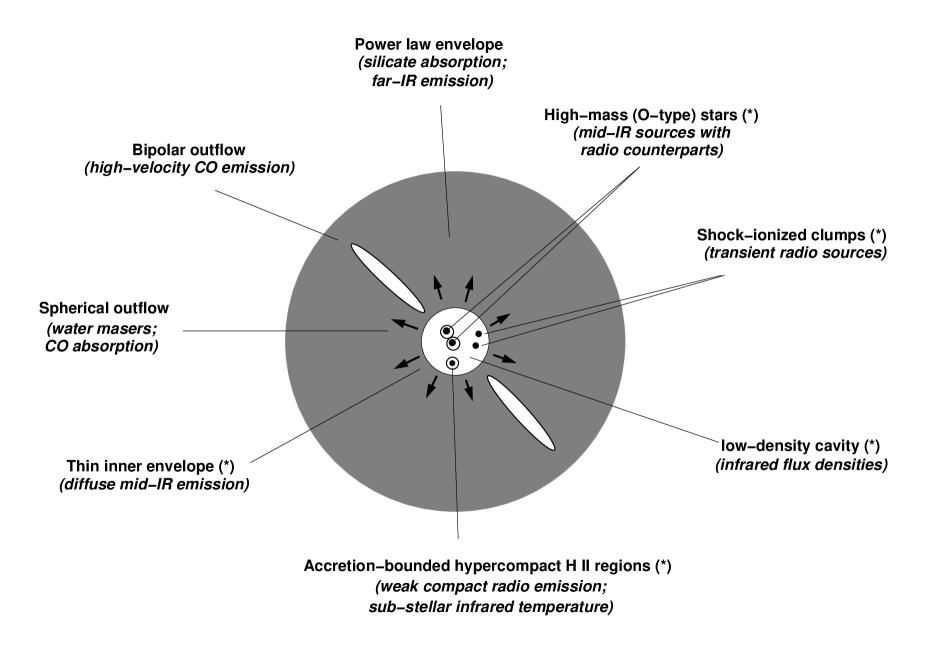
Figure 7: Schematic view of the W3 IRS5 region, as projected on the sky, with the observational characteristics of each physical component indicated. Asterisks mark new findings of this paper.

Observations at subarcsecond resolution at mid-infrared and radio wavelengths have led to a detailed picture of the W3 IRS5 region, shown schematically in Figure 7 and described below.

• The two bright mid-infrared sources with radio emission probably are deeply embedded high-mass stars. They are both close to groups of H₂O masers. The measured mid-infrared diameters are consistent with blackbody emission at $T$=390 K and providing all of the far-infrared luminosity of W3 IRS5.

• A third, weaker mid-infrared and radio source with associated H₂O masers is probably a somewhat later-type star which is energetically unimportant.

• Radio source A has an optically thick radio spectrum, and may have a counterpart at long mid-infrared wavelengths (${{}_{>}\atop{{}^{\sim}}}$17.65 $\mu$m). It may be an extremely deeply embedded high-mass star. The three power sources of W3 IRS5 then have $L$$\approx$40,000 L_⊙ each, which in the models of Maeder & Meynet (1989) makes them $\approx$20 M_⊙ stars (ZAMS spectral type O8).

• The region shows several transient radio sources. Some of these may represent runaway OB stars, but most are probably clumps in the ambient material which are ionized and destroyed by shocks with the winds of the O-type stars.

• The low silicate optical depth suggests that no underlying silicate emission is present. This is most easily explained by a cavity separating the high-mass stars from their envelope. Perhaps the cavity was blown by the slow spherical outflow traced by the H₂O masers.

• The far-infrared and submillimeter emission, as well as the low-velocity CO mid-infrared absorption, arise in the large-scale envelope. The dense stellar cluster visible in the near-infrared (and X-ray) is embedded in the same envelope.

In the future, subarcsecond monitoring of W3 IRS5 at high radio frequencies (VLA-A) is necessary to test the ‘proper motion’ and ‘shocked clump’ hypotheses. If proper motions are confirmed, the shapes of the orbits will be a test of the ‘runaway star’ hypothesis, and will constrain the dynamics of this young cluster. The emission mechanism should be studied by simultaneous observations at three or more wavelengths. If the e-VLA does not provide the sensitivity necessary to do this, ALMA will.

Mid-infrared imaging at wavelengths ${{}_{>}\atop{{}^{\sim}}}$20 $\mu$m at subarcsecond resolution is necessary to search for a mid-infrared counterpart to radio source Q2=K3=A. The main requirements are higher sensitivity and dynamic range than was achieved here; the higher angular resolution offered by MIDI on the VLTI will be more useful to search for fine structure. Spatially resolved mid-infrared spectroscopy is necessary to assign the high-velocity CO absorption features (Mitchell et al., 1991) to particular stellar components. This may be a good project for VLT/CRIRES. Future radiative transfer modeling efforts should consider broken power laws for the density distribution in the envelope of W3 IRS5.