Various applications of multicolour photometry and radial velocity data
for multimode $\delta$ Scuti stars

Abstract

In addition to revealing spherical harmonic degrees, $\ell$, of excited modes, pulsational amplitudes and phases from multicolour photometry and radial velocity data yield a valuable constraints on stellar atmospheric parameters and on subphotospheric convection. Multiperiodic pulsators are of particular interest because each mode yields independent constraints. We present an analysis of data on twelve modes observed in FG Vir star.

1 Introduction

In a recent paper Daszyńska-Daszkiewicz, Dziembowski, Pamyatnykh (2003, Paper I) showed that photometric amplitudes and phases of pulsating stars are useful not only to identify the spherical harmonic degree, $\ell$, but also for constraining models on stellar convection and stellar atmospheric parameters.

To calculate theoretical values of photometric amplitudes and phases we have to make use of the complex nonadiabatic parameter, $f$, which gives the ratio of the local flux perturbation to the radial displacement at the photosphere. The $f$ parameter is obtained from linear nonadiabatic calculation of oscillation in relevant stellar models. In the case of $\delta$ Scuti star models, $f$ is very sensitive to the treatment of subphotospheric convection. We also need models of stellar atmospheres for evaluation of the flux derivatives with respect to effective temperature and gravity and the limb-darkening coefficients. The most popular are Kurucz models (1998) but now there are alternative models available, e.g. Phoenix (Hauschildt et al. 1997) or NEMO.2003 (Nendwich et al. 2004).

In Paper I we proposed the method of extracting simultaneously $\ell$ and $f$ from multicolour data and applied it to several $\delta$ Scuti stars. In all cases the $\ell$ identification were unique and the inferred values of $f$ were sufficiently accurate to yield a useful constraints on convection. In the follow-up paper (Daszyńska-Daszkiewicz et al. 2004), we included radial velocity measurements, which improved significantly the determination of $\ell$ and $f$. The very important feature of this method is that we can determine the $\ell$ values in $\delta$ Scuti stars avoiding major theoretical uncertainty concerning subphotospheric convection.

Multimode pulsators are of special interest because each mode gives us independent constraints on stellar parameters. FG Vir is the most multimodal $\delta$ Scuti pulsator. After last photometric and spectroscopic campaigns the total number of detected modes increased up to 48 (Breger et al. 2004, Zima et al. 2004). For twelve frequencies we have both two-colour Strömgren photometry $(v,y)$, as well as radial velocity data. We apply our method to these modes using various models of stellar atmospheres.

2 Observations

Two recent photometric campaigns on FG Vir took place in 2002 and 2003. Spectroscopic observations were carried out in 2002. In Fig.1 we show how amplitudes and phases change from season 2002 to season 2003. We can see that for some of the modes, the differences are significant. This problem is more evident if we combine photometry and spectroscopy. In Fig.2 we present diagnostic diagrams for the spherical harmonic degree, $\ell$, constructed from photometric and spectroscopic observables. The conclusion is that only contemporaneous observations can be used.

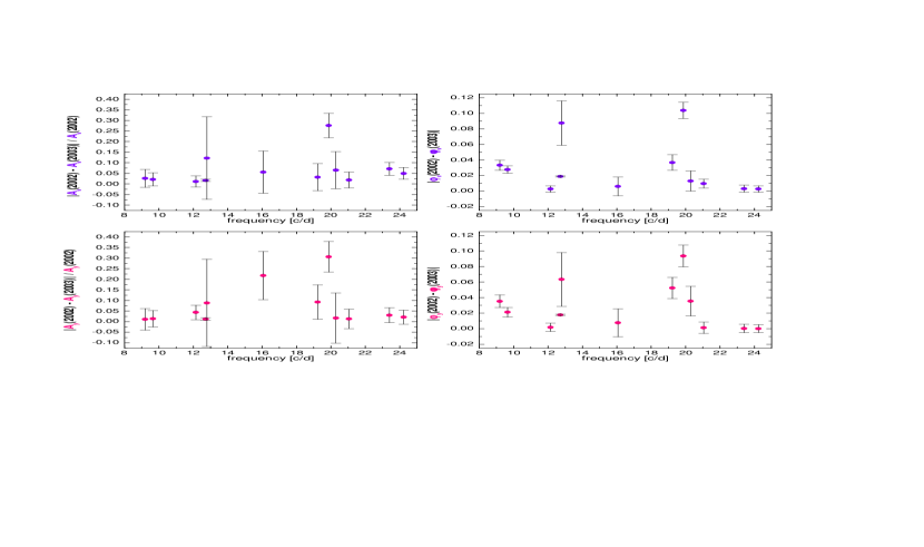
Figure 1: Changes in photometric amplitudes and phases between 2002 and 2003.

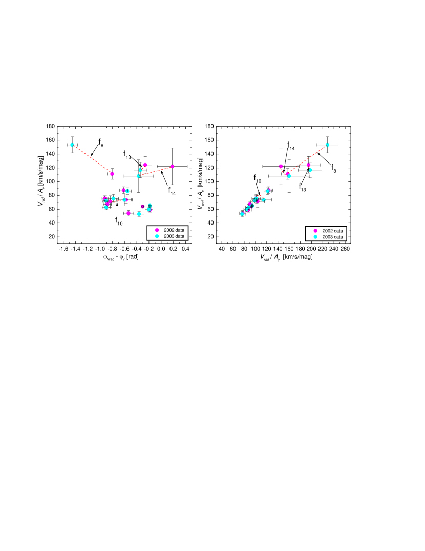
Figure 2: Diagnostic diagrams for the spherical harmonic degree, $\ell$, using combined photometric and spectroscopic data.

3 Method of inferring $\ell$ and $f$ from observations

The method is described in detail in Paper I. Here we give only a brief outline.

The complex photometric amplitudes for a number of passbands, $\lambda$, are written in the form of the linear observational equations

$${\cal D}_{\ell}^{\lambda}({\tilde{\varepsilon}}f)+{\cal E}_{\ell}^{\lambda}{\tilde{\varepsilon}}=A^{\lambda},$$ (1)

where

$${\tilde{\varepsilon}}=\varepsilon Y^{m}_{\ell}(i,0),$$ (2)

$${\cal D}_{\ell}^{\lambda}=\frac{1}{4}b_{\ell}^{\lambda}\frac{\partial\log({\cal F}_{\lambda}|b_{\ell}^{\lambda}|)}{\partial\log T_{\rm{eff}}}$$ (3)

$${\cal E}_{\ell}^{\lambda}=b_{\ell}^{\lambda}\left[(2+\ell)(1-\ell)-\left(\frac{\omega^{2}R^{3}}{GM}+2\right)\frac{\partial\log({\cal F}_{\lambda}|b_{\ell}^{\lambda}|)}{\partial\log g}\right]$$ (4)

Having spectroscopic observations we can supplement the above set with an expression for the radial velocity (the first moment, ${\cal M}_{1}^{\lambda}$)

$${\rm i}\omega R\left(u_{\ell}^{\lambda}+\frac{GM}{R^{3}\omega^{2}}v_{\ell}^{\lambda}\right){\tilde{\varepsilon}}={\cal M}_{1}^{\lambda}$$ (5)

Symbols in Eqs. (3.3-5) have the following meaning. $\varepsilon$ is a complex parameter fixing mode amplitude and phase, $i$ is inclination angle, and $b_{\ell}^{\lambda},~{}u_{\ell}^{\lambda},~{}v_{\ell}^{\lambda}$ are limb-darkening-weighted disc averaging factors. ${\cal F}(T_{\rm eff},g)$ is the monochromatic flux from static atmosphere models. Mean atmospheric parameters, ($T_{\rm eff},\log g,$ [m/H]), enter through ${\cal D}_{\ell}^{\lambda}$, ${\cal E}_{\ell}^{\lambda}$ and through the disc averaging factors, which contain the limb-darkening coefficients.

In the calculations reported in this paper, we used ${\cal F}_{\lambda}(T_{\rm eff},\log g,[m/H])$ from the Kurucz, Phoenix, and NEMO.2003 models. The limb-darkening coefficients were taken from Claret (2000, 2003) for the Kurucz and Phoenix models, and from Barban et al. (2003) for the NEMO.2003 models.

Each passband, $\lambda$, yields r.h.s. of equations (3.1). Measurements of radial velocity yield r.h.s. of equation (3.5). With data from two passbands we have three complex linear equations for two complex unknowns: ${\tilde{\varepsilon}}$ and $({\tilde{\varepsilon}}f)$ (note that $|\varepsilon f|$ is the relative amplitude of the luminosity variations). The equations are solved by LS method for specified $\ell$ values. The $\ell$ determination is based on the behavior of minima of $\chi^{2}(\ell)$. The inferred $f$ values are of interest as constraints on stellar convection models (Paper I).

4 Application to FG Vir

FG Vir is a well known $\delta$ Scuti variable located in the middle of its Main Sequence evolution. The basic stellar parameters, as derived from mean photometric indices and Hipparcos parallax, are: $\log T_{\rm eff}=3.875\pm 0.009$, $\log g=4.0\pm 0.1$. The mass estimated from evolutionary tracks is $M=1.85\pm 0.1M_{\odot}$. As was shown by Mittermayer & Weiss (2003), FG Vir has the solar chemical composition, thus in our calculations we adopt the standard metal abundance $Z=0.02$.

4.1 Identification of spherical harmonic degree, $\ell$

We applied the method to twelve frequencies of FG Vir. All of them have both photometric and spectroscopic data. We use only observations from 2002 because radial velocity measurements are only from 2002. In the present application the radial velocity data are essential because we have data for only two photometric passbands and three is the minimum if we want to rely on the pure photometric version of our method.

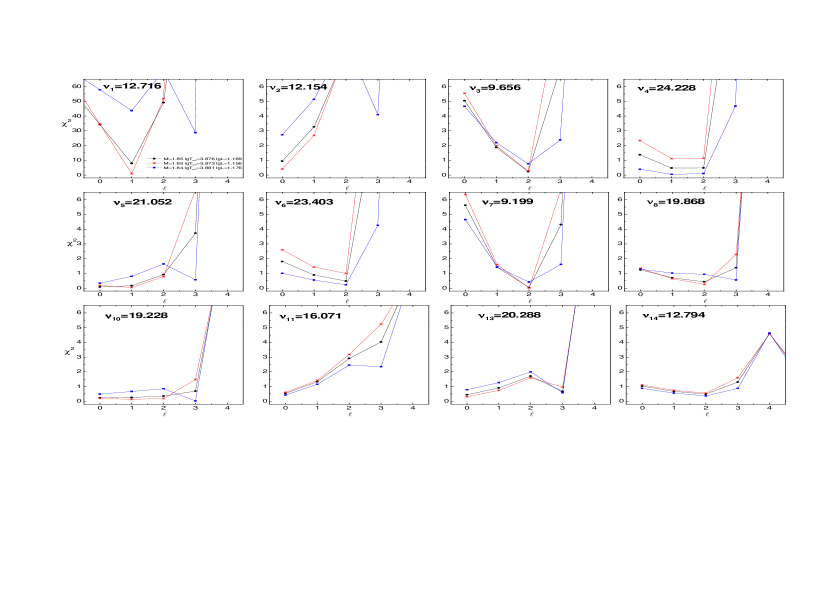
Figure 3: The values of $\chi^{2}$ from the method described in the text as a function of $\ell$.

Table 1: Possible identification of $\ell$ ($\chi^{2}\leq 1.6$) within the accepted $T_{\rm eff}$ range

$\nu$ [c/d]	our identification	Breger et al.	Viscum et al.	Breger et al.
	from phot.&spec.	(1995)	(1998)	(1999)
$\nu_{1}$= 12.7164	$\ell=1$	$\ell=0$	$\ell=1$	$\ell=1$
$\nu_{2}$= 12.1541	$\ell=0$	$\ell=2$	$\ell=0$	$\ell=0$
$\nu_{3}$= 9.6563	$\ell=2$	$\ell=2$	$\ell=2$	$\ell=1,2$
$\nu_{4}$= 24.2280	$\ell=2,1,0$	$\ell=0$	$\ell=1$	$\ell=1,2$
$\nu_{5}$= 21.0515	$\ell=1,0,2$	$\ell=1$	$\ell=2$	$\ell=2$
$\nu_{6}$= 23.4033	$\ell=2,1,0$	$\ell=2$	$\ell=0$	$\ell=0,1$
$\nu_{7}$= 9.1991	$\ell=2,1$	$\ell=2$	$\ell=2$	$\ell=2$
$\nu_{8}$= 19.8676	$\ell=2,1,0$	$\ell=2$	$\ell=2$	$\ell=2$

In Fig. 3 we plot $\chi^{2}$ as a function of $\ell$. The results were obtained using Kurucz models. We see that the discrimination of the $\ell$’s is sometimes better, sometimes worse. A unique $\ell$ identification is possible only for the highest amplitude modes. In Table 1 we compare our $\ell$ identifications with earlier ones. Clearly, we are less optimistic than our predecessors. We rejected only the $\ell$ values leading to $\chi^{2}\geq 1.6$. With this criterion we could assign a unique $\ell$ values only to three highest peeks. It is significant that $\ell>3$ is excluded in all twelve cases at the safe confidence level.

4.2 Constraints on stellar convection

In Fig. 4 we compare empirical values of parameters $f$ deduced from the data with the values obtained from linear nonadiabatic calculation. Here we rely on a rather naive treatment of convection: mixing-length theory (MLT) and convective flux freezing approximation.

The empirical $f$’s depend only weakly on adopted values of $T_{\rm eff}$ and $L$. The plotted values were obtained for $M=1.85M_{\odot}$, $\log T_{\rm eff}=3.873$ and $\log L=1.156$. These parameters are consistent with mean photometric data for FG Vir and evolutionary models, and they lead for the three highest amplitude modes to the lowest $\chi^{2}$ obtain with our method. The empirical $f$’s are relatively insensitive also to the choice of $\ell$ which in some cases is ambiguous. For the plot we use $\ell$’s corresponding to $\chi^{2}$ minimum. The calculated $f$’s are even less $\ell$-dependent.

We can see not a bad agreement with theoretical values of the $f$ parameter for models calculated with $\alpha=0.0$. This is good because our approximations are relevant in the limit of totally inefficient convection.

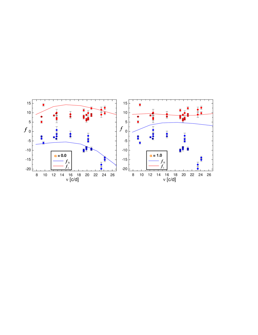
Figure 4: Comparison of empirical values of nonadiabatic parameter, $f$, (dots with error bars) with the theoretical ones calculated for two values of MLT parameter, $\alpha$.

4.3 Consequences of using different models of stellar atmospheres

Our determination of $\ell$ and $f$ requires atmospheric models. All our results so far were obtained with the use of Kurucz tabular data. In our comparison we use the data from Phoenix and NEMO.2003 models. Such a comparison is important for assessing reliability of the quoted $\ell$ and $f$ values. Models of stellar atmospheres are needed for evaluation coefficients ${\cal D}_{\ell}^{\lambda}$, ${\cal E}_{\ell}^{\lambda}$ and $b_{\ell}^{\lambda}$. The most important quantity derived from the models is the temperature derivative of the monochromatic flux

$$\alpha_{T}=\frac{\partial\log{\cal F}_{\lambda}}{\partial\log T_{\rm eff}},$$ (6)

which enters ${\cal D}_{\ell}^{\lambda}$. This quantity depends most strongly on $T_{\rm eff}$ and the same must be true for the minimum $\chi^{2}$. This suggest that the best value of $T_{\rm eff}$ in the same as the best value of $\ell$.

We found that relying on different atmospheric models, the $\ell$ identification based on $\chi^{2}$ minima is unchanged but the minimum values of $\chi^{2}$ in the accepted $T_{\rm eff}$ range were much larger than the ones obtained with the use of Kurucz data. We then relaxed the temperature constraint and considered models in a wide range of $T_{\rm eff}$. We use the fit of $\nu_{2}$ to the radial fundamental mode and evolutionary tracks to derive corresponding value of $\log g$. We encountered two problems, which are illustrated in Fig.5:

• acceptable minima of $\chi^{2}$ for Phoenix and NEMO.2003 models were found outside the acceptable $T_{\rm eff}$ range

• in Kurucz and Phoenix models the temperature flux derivatives, $\alpha_{T}$, are non-smooth which gives bad shape of $\chi^{2}(T_{\rm eff})$

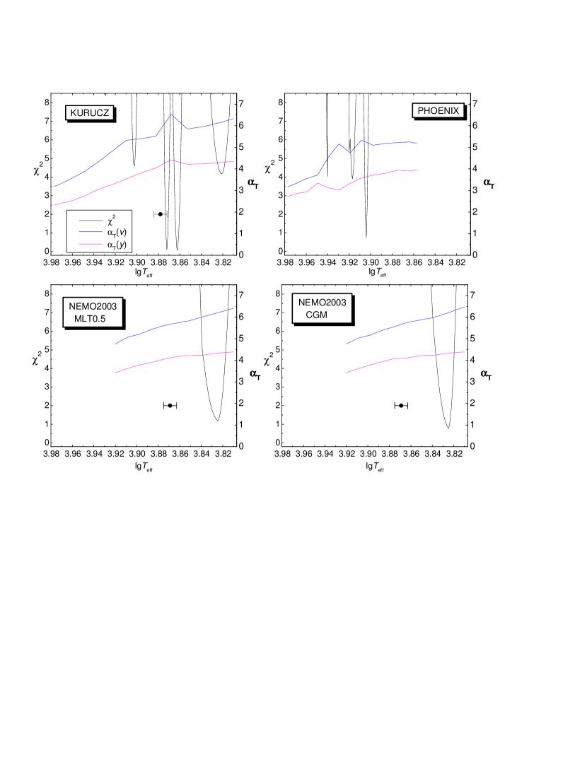
Figure 5: $\chi^{2}$ as a function of effective temperature a the dominant mode, $\nu_{1}$. Dots with error bars show the values derived from mean colors.

5 Conclusions

A unique identification of spherical harmonic degree, $\ell$, of excited modes without a priori knowledge of complex parameter $f$, which links the surface flux variation to displacement, is possible. However, in the case of low amplitude modes, more accurate observations and measurements in more passbands are needed.

The values of $f$ inferred from data for FG Vir are crudely consistent with models calculated assuming inefficient convection $(\alpha\approx 0.0)$. We showed that there is a prospect for constraining $T_{\rm eff}$ from the pulsation data. However, for this application we need more accurate derivatives of the fluxes in various passbands with respect to $T_{\rm eff}$ than the derivatives we may calculated from available tables of atmospheric models.

There are indeed various applications of amplitude and phase data from photometric and spectroscopic observations of pulsating stars. Multimode pulsators are advantageous, but the mode amplitudes have to be determined with a high accuracy. Data from photometric observations in more than two passbands are very much desired.