Eighth-Order Image Masks For Terrestrial Planet Finding

Abstract

We describe a new series of band-limited image masks for coronagraphy that are insensitive to pointing errors and other low-spatial-frequency optical aberrations. For a modest cost in throughput, these “eighth-order” masks would allow the Terrestrial Planet Finder Coronagraph (TPF-C) to operate with a pointing accuracy no better than that of the Hubble Space Telescope. We also provide eighth-order notch filter masks that offer the same robustness to pointing errors combined with more manageable construction tolerances: binary masks and sampled graded masks with moderate optical density requirements.

1 INTRODUCTION

Coronagraphy holds great promise for imaging extrasolar planetary systems, even extrasolar terrestrial planets only $\sim 10^{-10}$ times as bright as their host stars (e.g. Kuchner & Spergel, 2003a). However, finding extrasolar terrestrial planets at contrast levels of $\sim 10^{-10}$ using any of the present image mask designs requires either pointing accuracies at the level of a fraction of a milliarcsecond (Kuchner & Traub, 2002; Kuchner & Spergel, 2003b) or apodization in the pupil plane (e.g. Aime et al., 2002; Kasdin et al., 2003), which generally carries a high penalty in throughput and inner working angle (but see also Guyon, 2003; Traub & Vanderbei, 2003). We offer a new series of band-limited image masks that can provide high contrast levels without pupil apodization because they are intrinsically insensitive to pointing errors and other low-order aberrations. We also provide notch filter versions of these masks that may be easier to build to the necessary tolerances.

2 EIGHTH-ORDER MASKS

2.1 Band-limited Masks and Notch Filter Masks

Here we summarize the basic definitions of band-limited masks and notch filter masks stated by Kuchner & Traub (2002); Kuchner & Spergel (2003b). We will focus on linear masks, described by functions of a single variable, $x$. One-dimensional band-limited and notch filter masks can be combined to create a wide variety of two-dimensional masks.

An ideal linear image mask can be described by a function, $\hat{M}(x)$, called the mask function. In our simple model of the interaction between masks and light, the mask function, also called the mask’s amplitude transmissivity, multiplies the electric field phasor of the incoming beam. The intensity transmissivity of a mask, $|\hat{M}({x})|^{2}$, multiplies the intensity of the beam. We will also refer often to the mask function, the mask intensity transmissivity, and to the Fourier transform of the mask function,

$$M(u)=\int\hat{M}(x)\,e^{-2\pi iux}\,dx.$$ (1)

Kuchner & Traub (2002) showed that if $\hat{M}({x})$ is a notch filter function, i.e.,

$$M(u)=0\quad\mbox{for}\,\,\epsilon/2<|u|<1-\epsilon/2,$$ (2)

where $\epsilon$ sets the undersizing of the Lyot stop, and if

$$\int_{-\epsilon/2}^{\epsilon/2}M(u)\,du=0,$$ (3)

then the mask defined by $\hat{M}(x)$ will completely remove all on-axis light in an ideal coronagraph with a uniform entrance pupil. Kuchner (2005) showed that notch filter masks are the only trivially achromatic masks that completely remove on-axis light in a one-dimensional or separable two-dimensional coronagraph. Masks we can construct without amplifying the beam or manipulating its phase are necessarily limited to $0\leq\hat{M}(x)\leq 1$. A band-limited mask is a notch filter mask with $M(u)=0$ for $|u|>\epsilon/2$.

We aim to find notch filter mask functions, $\hat{M}(x)$, that provide deep suppression of light near the optical axis, not just at the optical axis. We will first derive new band-limited masks and then follow the recipes in Kuchner & Spergel (2003b) to generate useful notch-filter masks based on them.

2.2 Blocking Slightly-Off-Axis Light

Understanding the off-axis behavior of an ideal coronagraph with a band-limited mask is easy. A coronagraph with a band-limited image mask attenuates the intensity of an image of a point source located at an angle $x$ by a factor of $|\hat{M}(x)|^{2}$ compared to the image the source would have if the image mask were removed while the Lyot stop remained in place (see the Appendix). In an ideal coronagraph with a band-limited mask, the point spread function (PSF) is independent of the position of the source with respect to the optical axis; only the attenuation varies with $x$. Hence, we can describe the way a band-limited mask attenuates sources near the optical axis, including the target star, simply by expanding $\hat{M}(x)$ about $x=0$.

If the first important term in this expansion is quadratic in $x$, the intensity attenuation will vary as $x^{4}$. Borrowing the language of interferometry, we might say such a mask produces a fourth-order null. For a demonstration of why this interferometric terminology is appropriate, consider the nulling coronagraph described by Levine et al. (2003), which monochromatically synthesizes a particular band-limited mask with a fourth-order null using beam combiners.

All of the band-limited mask designs and notch filter mask designs illustrated in Kuchner & Traub (2002), Kuchner & Spergel (2003b), and Kuchner (2005) have fourth-order nulls. For example, all of the popular $1-\mbox{sinc}^{n}$ family of masks are fourth order; $1-\mbox{sinc}^{n}k_{1}x/n\approx(1/6n)(k_{1}x)^{2}$. But we can design band-limited masks and notch filter masks with nulls of any order, $\beta$, by the methods described below, if $\beta$ is a multiple of 4.

The order of the null dictates the sensitivity of the mask to optical aberrations that effectively spread the light from a target source around some region of the sky near the optical axis. Tip-tilt error (caused by pointing error, for example) is the simplest low-order aberration for us to model and a term that can easily dominate a coronagraph design’s error budget. A pointing error of $\Delta\theta$ will cause an intensity leak proportional to $(\Delta\theta)^{\beta}$. A mask that is insensitive to pointing error will also defeat other low-order aberrations like defocus, coma and astigmatism to some degree, though some low-order Zernike terms contain mid-spatial-frequency tails that may leak through. Mid-spatial-frequency errors are problematic for any coronagraph design because by definition they coincide with the search area; no mask or stop can block them without also blocking light from the planet. Shaklan & Green (2005) discuss the effects of low-order aberrations in a coronagraph with an eighth-order mask in detail.

The fractional leakage through a mis-pointed coronagraph with a band-limited mask is simply

$$L={{\int\int I(x+\Delta\theta,y)\,|\hat{M}(x,y)|^{2}\,dxdy}\over{\int\int I(x,y)\,dxdy}},$$ (4)

where $I(x,y)$ is the source intensity, i.e., the stellar disk, and $\Delta\theta$ is the instantaneous pointing error. For a fourth-order linear mask, the instantaneous fractional intensity leakage is

$$L={{\theta_{*}^{4}+48\,\theta_{*}^{2}(\Delta\theta)^{2}+128(\Delta\theta)^{4}}\over{256\,\theta_{IW}^{4}}},$$ (5)

where $\theta_{*}$ is the angular diameter of the star and $\theta_{IW}$ is the inner working angle of the mask, defined by $|\hat{M}(\theta_{IW})|^{2}=1/2$. To derive this expression, we made the approximation that $\hat{M}(x)=x^{4}$; we have corrected a numerical error in Equation 17 of Kuchner & Spergel (2003b). If we assume $\Delta\theta$ is distributed in a Gaussian with standard deviation $\sigma_{\Delta\theta}$, and $\sigma_{\Delta\theta}>>\theta_{*}$, then we find that the mean leakage is

$$\langle L\rangle=1.5(\sigma_{\Delta\theta}/\theta_{IW})^{4}.$$ (6)

So if we assume that we can tolerate a leakage of $\langle L\rangle<3\times 10^{-8}$, and that $\Delta\theta$ is much larger than the angular radius of the star, we find that we must center the star on the mask to an accuracy of

$$\sigma_{\Delta\theta}<0.012\,\theta_{IW}.$$ (7)

Though it is easiest to interpret in terms of pointing error, this Gaussian blurring can also serve as a crude model of the effects of other low-order aberrations.

For an eighth-order mask approximated as $\hat{M}(x)=x^{8}$, the instantaneous fractional intensity leakage is

$$L={{7\,\theta_{*}^{8}+1120\,\theta_{*}^{6}(\Delta\theta)^{2}+17920\,\theta_{*}^{4}(\Delta\theta)^{4}+57344\,\theta_{*}^{2}(\Delta\theta)^{6}+32768(\Delta\theta)^{8}}\over{65536\,\theta_{1/2}^{8}}},$$ (8)

the corresponding mean fractional leakage is

$$\langle L\rangle=52.5(\sigma_{\Delta\theta}/\theta_{1/2})^{8},$$ (9)

and the pointing requirement for leakage $\langle L\rangle<3\times 10^{-8}$ is

$$\sigma_{\Delta\theta}<0.070\,\theta_{IW},$$ (10)

a factor of $\sim 6$ improvement over the $\sigma_{\Delta\theta}$ tolerance for fourth-order masks. A coronagraph designed to find extrasolar terrestrial planets like the Terrestrial Planet Finder Coronagraph (TPF-C) might need $\theta_{IW}=60$ milliarcseconds (mas). This requirement implies a pointing tolerance of $\sigma_{\Delta\theta}\leq 0.72$ mas using a fourth-order mask or $\sigma_{\Delta\theta}\leq 4.2$ mas using an eighth-order mask. For comparison, the Hubble Space Telescope points to $\sigma_{\Delta\theta}\approx 3$ mas (Burrows et al., 1991).

Eighth-order masks can also provide high-contrast images of extended sources, though relaxing the pointing tolerance depletes some of this power. For a fourth-order mask, Equation 5 shows that the extent of a central source begins to matter when $\theta_{*}>(8/3)(\Delta\theta)$ and the cross term begins to dominate. For an eighth-order mask, Equation 8 shows that the extent of a central source begins to be important when $\theta_{*}>(4/7)(\Delta\theta)$. In the TPF-C example above, these limits correspond to $\theta_{*}=1.9$ mas for a fourth-order mask and $\theta_{*}=2.4$ mas for an eighth-order mask; a solar-type star at 10 pc is about 1 mas in diameter. In other words, a TPF-C design with an eighth-order mask may be slightly better suited for the closest target stars than one using with a fourth-order mask even with its relaxed pointing tolerance, depending on the wings of the actual distribution of pointing errors.

3 CONSTRUCTING THE MASKS

To design an eighth-order band-limited mask, we can create a linear combination of two fourth-order band-limited masks weighted so that the term responsible for the quadratic leak cancels; i.e.,

$$\left.{{d^{2}}\over{dx^{2}}}\hat{M}(x)\right|_{x=0}=0.$$ (11)

For example, we can add a term of the form $C(1-\cos(k_{2}x))$, otherwise known as a $\sin^{2}$ mask, to any $1-\mbox{sinc}^{n}$ mask to create a new mask with $d^{2}\hat{M}(x)/dx^{2}|_{x=0}$, while still satisfying Equation 3. If we start with a mask of the form $1-\mbox{sinc}^{n}k_{1}x/n\approx(k_{1}x)^{2}/(6n)$ and add $C(1-\cos(k_{2}x))\approx(C/2)(k_{2}x)^{2}$, we find that to produce an eighth order mask, we require that $C=-(1/3n)(k_{1}/k_{2})^{2}$.

However, we do not want to add a $\sin^{2}$ mask of just any random spatial frequency. We would prefer a frequency within the bandwidth of the original mask so that we don’t suffer an undue throughput penalty; i.e., $k_{2}$ needs to be $\leq k_{1}$. In order to minimize $|C|$, we should pick a frequency at exactly the edge of the band; i.e., $k_{2}=k_{1}$. With this constraint, we find $C=-1/(3n)$.

Of course, adding mask functions can violate the requirement that $\hat{M}(x)\leq 1$. To ensure $\hat{M}(x)\leq 1$, we can renormalize the mask by multiplying $\hat{M}(x)$ by a constant, $N$, equal to the inverse of its maximum value.

Putting everything together and using physical units yields a series of eighth-order band-limited masks,

$$\hat{M}_{BL}(x)=N\left[\frac{3n-1}{3n}-\mbox{sinc}^{n}{{\pi x\epsilon}\over{n\lambda_{max}f}}+\left({1\over{3n}}\right)\cos{{\pi x\epsilon}\over{\lambda_{max}f}}\right],$$ (12)

where $f$ is the focal ratio at the mask and $\lambda_{max}$ is the longest wavelength at which the mask is to operate. Figure 1 shows $\hat{M}(x)$ for the first few linear masks in the series. The $n=3$ design offers a good compromise between the large sidelobes of the $n=1$ mask and the higher inner working angle-bandwidth product of the $n=5$.

The ringing in these image masks reduces their effective throughputs. The amplitude of the additional ringing introduced by the cosine term in Equation 12 falls off slowly with $n$, so simply increasing $n$ does not help much.

Fortunately, we can create another series of eighth-order masks with less ringing by combining two $1-\mbox{sinc}^{n}$ masks instead of a $1-\mbox{sinc}^{n}$ mask and $\sin^{2}$ mask using the same procedure we used to construct Equation 12:

$$\hat{M}_{BL}(x)=N\left[\frac{l-m}{l}-\mbox{sinc}^{l}{{\pi x\epsilon}\over{l\lambda_{max}f}}+\frac{m}{l}\,\mbox{sinc}^{m}{{\pi x\epsilon}\over{m\lambda_{max}f}}\right].$$ (13)

This series of masks has less ringing than the series described by Equation 12. It is parametrized by two integer exponents, $l$ and $m$; we assume $l>m$. Figure 2 shows $\hat{M}(x)$ for $m=1$ and $l=$2–5. The $m=1$ and $l=$2–3 masks have throughput similar to the $n=3$ cosine mask. Using large values of $m$ and $l$ reduces the ringing further, but it also reduces the Lyot stop throughput.

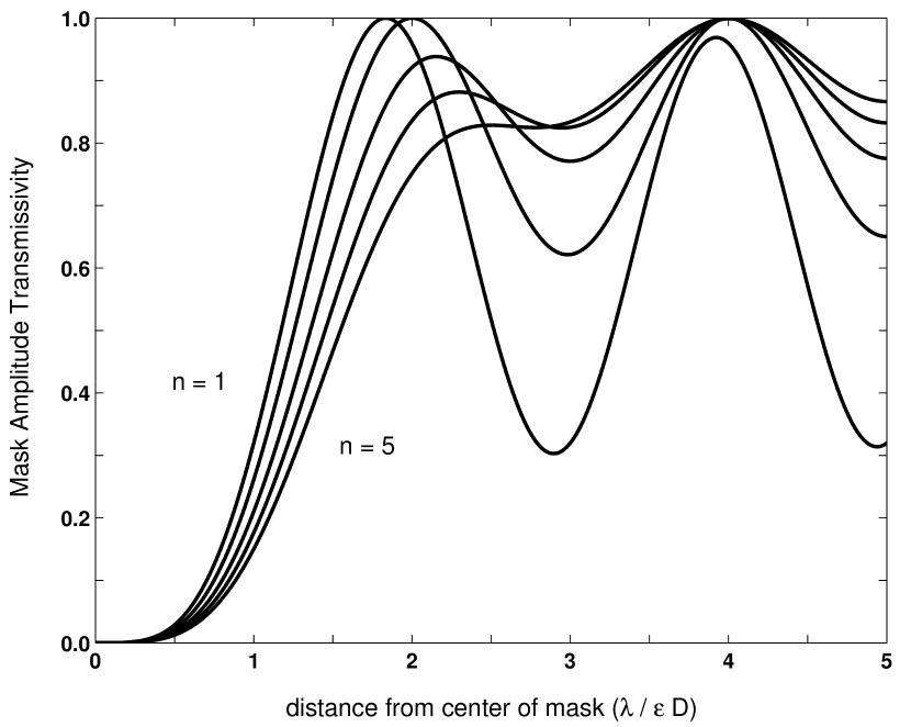
Figure 1: Eighth-order band-limited mask functions described by Equation 12 for $n=1-5$.

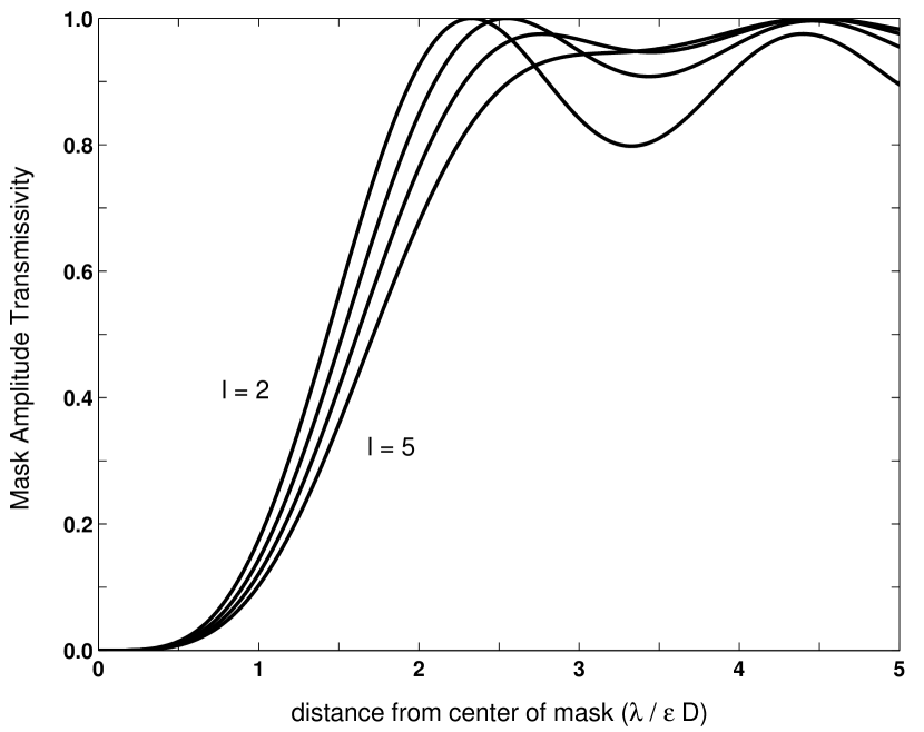
Figure 2: Eighth-order band-limited mask functions described by Equation 13 for $m=1$, $l=2-5$.

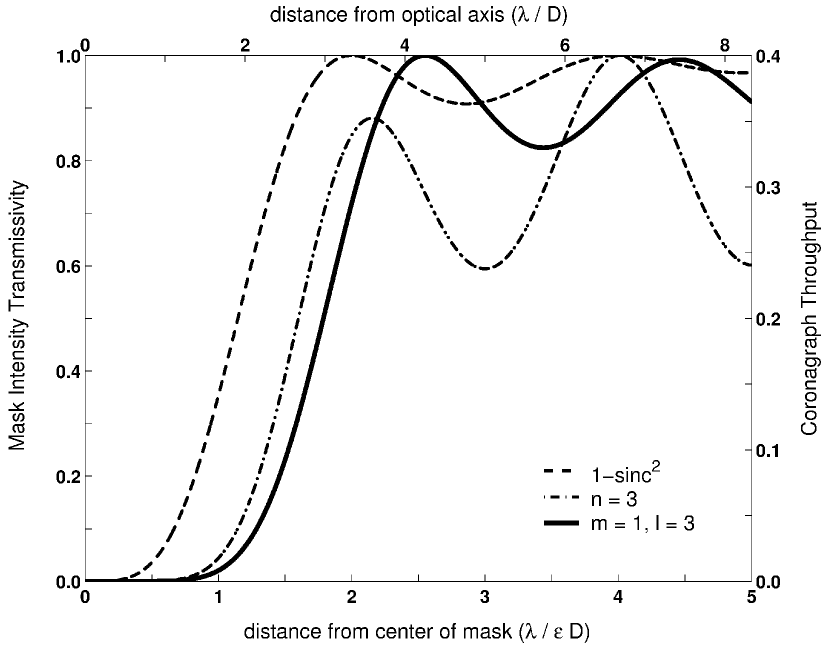
Figure 3: Intensity transmissivities for the $1-\mbox{sinc}^{2}$ fourth-order mask, the $n=3$ eighth-order mask, and the $m=1$, $l=3$ eighth-order mask. Coronagraph throughput and distance from optical axis were calculated with $\epsilon=0.6$. The $m=1$, $l=3$ eighth-order mask, recommended for TPF-C, has 100% transmissivity at its first maximum.

Figure 3 compares the intensity transmissivity, $|\hat{M}(x)|^{2}$, for the $1-\mbox{sinc}^{2}$ fourth-order mask and the $m=1$, $l=3$ eighth-order mask. While the $1-\mbox{sinc}^{2}$ mask has an inner working angle of $\theta_{IW}=(1.448/\epsilon)(\lambda/D)$, the $m=1$, $l=3$ eighth-order mask has an inner working angle of $\theta_{IW}=(1.788/\epsilon)(\lambda/D)$. The $m=1$, $l=3$ mask offers a good compromise between ringing and throughput, and also reaches 100% transmissivity at its first maximum, a critical region for planet searching; we recommend this mask for TPF-C.

Consider a TPF-C design with $\theta_{IW}=3\,\lambda/D$ using a linear fourth-order mask. This coronagraph has a bandwidth of $\epsilon=0.4$ and a nominal Lyot stop throughput of $1-\epsilon=0.6$ (see Kuchner & Spergel, 2003b). This fourth-order design probably requires some mild apodization of the Lyot stop to ameliorate leakage due to low-order optical aberrations, reducing the throughput to $0.35$. Keeping $\theta_{IW}=3\,\lambda/D$ but switching to a linear $m=1$, $l=3$ eighth-order mask would mean working at a bandwidth of $\epsilon=0.596$ and a Lyot stop throughput of $1-\epsilon=0.404$. Coronagraphs with eighth-order masks should not require any Lyot stop apodization.

In other words, our analysis suggests that eighth-order masks combined with un-apodized Lyot stops perform about as well as fourth-order masks combined with apodized Lyot stops in terms of throughput and robustness to pointing errors. An alternative way to provide robustness to pointing errors is to use a shaped-pupil coronagraph (Kasdin et al., 2003; Vanderbei et al., 2003a, b). But the throughput offered by an eighth-order linear mask is still better than the typical throughput of a shaped pupil coronagraph at a given inner working angle, particularly when a shaped pupil coronagraph is used with a hard-edged image mask, which increases its effective inner working angle (Kuchner, 2005).

4 EIGHTH-ORDER NOTCH FILTER MASKS

The functions described by Equations 12 and 13 can be used in a variety of ways, e.g., to make linear masks ($\hat{M}(x,y)=\hat{M}_{BL}(x)$), radial masks ($\hat{M}(r)=\hat{M}_{BL}(r)$), or separable masks ($\hat{M}(x,y)=\hat{M}_{BL}(x)\hat{M}_{BL}(y)$). However, all band-limited masks are necessarily smooth graded masks. Notch-filter masks offer even more design freedom and need not necessarily be smooth, making them potentially easier to manufacture than band-limited masks (Kuchner & Spergel, 2003b).

Notch filter masks affect starlight and planet-light the same way as band-limited masks; only their low-spatial frequency parts contribute to starlight suppression. Consequently, in an eighth-order notch filter mask, only the low-frequency part needs to satisfy Equation 11. In other words,

$$\left.{{d^{2}}\over{dx^{2}}}\left(\mbox{the low-frequency part of}\ \hat{M}(x)\right)\right|_{x=0}=\int_{-\epsilon/2}^{\epsilon/2}(-2\pi iu)^{2}M(u)\,du=0.$$ (14)

Equivalently, we can say that an eighth-order notch filter mask satisfies Equations 2, 3, and also

$$\int_{-\epsilon/2}^{\epsilon/2}u^{2}M(u)\,du=0.$$ (15)

To find masks that meet these criteria, we can use a technique similar to the one employed in $\S$3. Since any linear combination of fourth-order notch filter mask functions will automatically satisfy Equations 2 and 3, we will start by writing

$$\hat{M}_{notch_{8}}(x)=N\left[\hat{M}_{notch_{4A}}(x)+C\hat{M}_{notch_{4B}}(x)\right],$$ (16)

where $\hat{M}_{notch_{4A}}(x)$ and $\hat{M}_{notch_{4B}}(x)$ represent different fourth-order notch filter mask functions and $N$ ensures that $\hat{M}_{notch_{8}}(x)\leq 1$. To construct a notch filter mask that exhibits eighth-order behavior, we need to weight the linear combination so that the new notch filter function also satisfies Equation 15. In other words we will find the constant $C$ by substituting Equation 16 into 15.

$$C=-\frac{\int_{-\epsilon/2}^{\epsilon/2}u^{2}M_{notch_{4A}}(u)\,du}{\int_{-\epsilon/2}^{\epsilon/2}u^{2}M_{notch_{4B}}(u)\,du}.$$ (17)

This constant should be negative; it should also satisfy $|C|<1$

By combining fourth-order notch filter functions and using the solutions to Equation 17, we can construct a variety of eighth-order notch filter masks analogous to the variety of eighth-order band-limited masks. For example, we can make a family of eighth-order notch filter masks using the $1-\mbox{cos}$ and $1-\mbox{sinc}^{n}$ fourth-order notch filter functions. We can also design low-ringing eighth-order notch filter masks using the $1-\mbox{sinc}^{m}$ and $1-\mbox{sinc}^{l}$ notch filter functions. To be consistent with $\S$3, we will refer to the various eighth-order notch filter masks by the exponents of their constituent functions ($n$, $m$, $l$, … etc.). In the following, we provide example calculations for making eighth-order binary and graded notch filter masks using the $m=1$, $l=3$ design.

4.1 Eighth-order Binary Masks

Notch filter masks can be designed to be binary: everywhere either completely opaque or completely transparent. A simple way to make such a binary mask is to assemble a mask from a collection of identical parallel stripes, where any arbitrary notch filter mask function provides the width of each stripe. In other words, each stripe is defined by

$$\hat{M}_{stripe}(x,y)=\left\{\begin{array}[]{ll}1&\mbox{where}\,\,y<\hat{M}_{notch}(x)\,\lambda_{min}f\\ 0&\mbox{elsewhere}.\end{array}\right.$$ (18)

and the mask function is

$$\hat{M}_{binary}(x,y)=\sum_{j=-\infty}^{\infty}\hat{M}_{stripe}(x,\;y-j\lambda_{min}f),$$ (19)

where $\lambda_{min}$ is the shortest wavelength in the band of interest.

If we like, we can use the band-limited mask functions described by Equations 12 or 13 in place of $\hat{M}_{notch}(x)$, resulting in a mask formed of continuous curves. However, sampled binary masks may prove to be easier to manufacture since their features are not as small near the optical axis. We will construct here an eighth-order sampled binary mask. Such a mask can be made entirely from rectangles of opaque material. Debes et al. (2004) have demonstrated the construction of sampled fourth-order masks using e-beam lithography.

Fourth-order sampled masks are defined by the following prescription (Kuchner & Spergel, 2003b):

$$\hat{M}_{notch_{4}}(x)=\hat{M}_{samp_{4}}(x)-\hat{M}_{0},$$ (20)

where

$$\hat{M}_{samp_{4}}(x) = \hat{P}(x)*\left(\hat{M}_{BL_{4}}(x)\,{\Delta x}\sum_{k}\delta(x-(k+\zeta)\Delta x)\right),$$ (21a)

$$M_{samp_{4}}(u) = P(u)\left(M_{BL_{4}}(u)*\sum_{k}\delta(u-k/\Delta x)e^{-2\pi iu\zeta\Delta x}\right),$$ (21b)

and

$$\hat{M}_{0}=\int_{-\epsilon D/(2\lambda)}^{\epsilon D/(2\lambda)}M_{samp_{4}}(u)\,du=\int_{-\infty}^{\infty}M_{BL_{4}}(u)P(u)\,du=\left.\hat{M}_{BL_{4}}(x)*\hat{P}(x)\right|_{x=0}.$$ (22)

Here, $M_{BL_{4}}$ represents any fouth-order band-limited mask function, $k$ ranges over all integers, and $*$ indicates convolution. The sampling points are offset from the mask center by a fraction $\zeta$ of $\Delta x$. The kernel, $\hat{P}(x)$, can represent the “beam” of a nanofabrication tool. It should be normalized so that $\int_{-\infty}^{\infty}\hat{P}(x)\,dx=1$, and $\hat{P}(x)$ must be everywhere $\leq 1/(\Delta x)$, so $\hat{M}_{samp_{4}}(x)$ remains $\leq 1$. The constant $\hat{M}_{0}$ ensures that the mask satisfies Equation 3. Though the sampled mask is derived from $\hat{M}_{BL_{4}}(x)$, the function being sampled is $\hat{M}_{BL_{4}}(x)-\hat{M}_{0}$.

Combining Equation 16 and Equation 20, we have

$$\hat{M}_{notch_{8}}(x) = N\left[\hat{M}_{notch_{4A}}(x)+C\hat{M}_{notch_{4B}}(x)\right]$$ (23)

$$= N\left[(\hat{M}_{samp_{4A}}(x)-\hat{M}_{0_{A}})+C(\hat{M}_{samp_{4B}}(x)-\hat{M}_{0_{B}})\right],$$ (24)

where $\hat{M}_{samp_{4A,B}}(x)$ are sampled versions of the fourth-order band-limited functions $\hat{M}_{BL_{4A,B}}(x)$ described by Equation 21b. The constants $\hat{M}_{0_{A,B}}$ and $C$ ensure that $\hat{M}_{notch_{4A,B}}(x)$ satisfy both Equation 3 and Equation 15, The constant $C$ is given by

$$C=-\frac{\int_{-\epsilon/2}^{\epsilon/2}u^{2}P(u)M_{BL_{4A}}(u)\,du}{\int_{-\epsilon/2}^{\epsilon/2}u^{2}P(u)M_{BL_{4B}}(u)\,du}.$$ (25)

To make an eighth-order sampled notch filter mask, the function that we sample is $N[(\hat{M}_{BL_{4A}}(x)-\hat{M}_{0_{A}})+C(\hat{M}_{BL_{4B}}(x)-\hat{M}_{0_{B}})]$.

Figure 4 shows a plot of the function $N[(\hat{M}_{BL_{4A}}(x)-\hat{M}_{0_{A}})+C(\hat{M}_{BL_{4B}}(x)-\hat{M}_{0_{B}})]$ to illustrate how $\zeta$ may be chosen. This example uses the $m=1$, $l=3$ sampled eighth-order mask, meaning $\hat{M}_{BL_{4A}}(x)=1-\mbox{sinc}(x)$ and $\hat{M}_{BL_{4B}}(x)=1-\mbox{sinc}^{3}(x)$. To guarantee that $\hat{M}_{notch}(x)\geq 0$, the parameter $\zeta$ must be in the range $|\zeta|\leq\zeta_{0}$, where $\zeta_{0}$ is defined by the condition $\hat{M}_{BL_{4A}}(\zeta_{0}\lambda_{min}f)+C\hat{M}_{BL_{4B}}(\zeta_{0}\lambda_{min}f)=\hat{M}_{0_{A}}+C\hat{M}_{0_{B}}$. For our binary mask, we will choose $\zeta=\zeta_{0}$, to make the central rectangles contiguous.

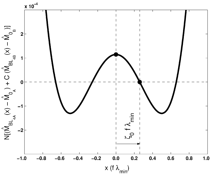
Figure 4: An example of the function $N[(\hat{M}_{BL_{4A}}(x)-\hat{M}_{0_{A}})+C(\hat{M}_{BL_{4B}}(x)-\hat{M}_{0_{B}})]$ for an $m=1$, $l=3$ sampled mask. Choosing $\zeta=\zeta_{0}$ allows us to create a binary mask of contiguous stripes. Choosing $\zeta=0$ allows us to create a graded mask with the most favorable optical density requirement.

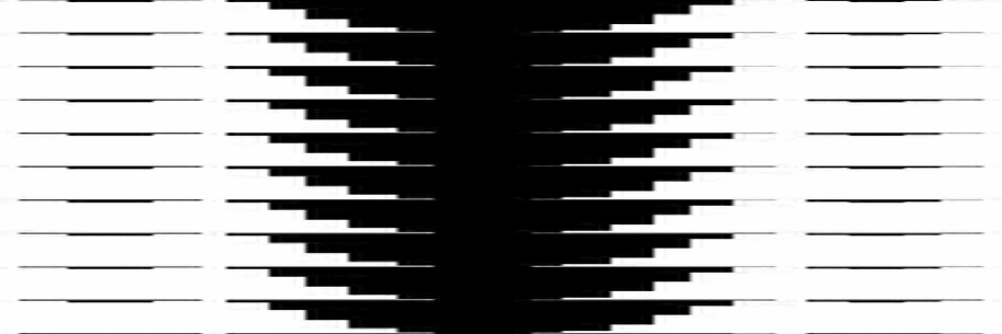
Figure 5: Simulated high magnification picture of an $m=1$, $l=3$ linear eighth-order sampled binary mask. Dark areas are completely opaque and white areas perfectly transmissive. See Debes et al. (2004) for optical microscope photographs of an actual linear fourth-order 1-sinc² binary mask.

The bandwidth of a mask should be chosen conservatively; e.g., $\lambda_{max}$ should be somewhat larger then the longest wavelength where the detector is sensitive so a filter with a finite slope can remove all the extraneous light. Band-limited masks and notch filter masks leak light at wavelengths longer than $\lambda_{max}$; notch filter masks also leak light at wavelengths shorter than $\lambda_{min}$. At a fixed inner working angle, increasing $\lambda_{max}$ necessitates increasing $\epsilon$, and thereby decreasing the throughput. Decreasing $\lambda_{min}$ means spacing the stripes and samples in a notch filter mask closer together.

For the $m=1$, $l=3$ mask with $\theta_{IW}=3\,\lambda_{max}/D$, spacing $\Delta x=\lambda_{min}f$, and bandpass 0.5–0.8 $\mu$m, we find that $\hat{M}_{0_{A}}=0.00630889$, $\hat{M}_{0_{B}}=0.01882618$, $C=-0.33935486$, and $\zeta_{0}=0.25941279$. Table 1 lists normalization constants and sampled mask parameters for eighth-order notch filter masks of various inner-working-angles using a top-hat kernel, $\hat{P}(x)=(D/\lambda_{min})\Pi(xD/\lambda_{min})$, and 0.5–0.8 $\mu$m bandpass.

If the resolution of our nanotool is $\sim\;$20 nm, we require a telescope with an f/115 or slower beam (see Kuchner & Spergel, 2003b). The physical size of an entire mask is generally a few hundred diffraction widths. A 1” $\times$ 1” mask would consist of $\gtrsim 440$ vertically repeating segments, where each segment is $\leq\lambda_{min}f=57.5\;\mu m$ wide. This coronagraph design would have a Lyot stop throughput of 40%. Figure 5 shows an example of what an $m=1$, $l=3$ linear eighth-order binary mask would look like.

A similar mask can also be made by replacing Equation 18 with

$$\hat{M}_{stripe}(x,y)=\left\{\begin{array}[]{ll}1&\mbox{where}\,\,|y|<\hat{M}_{notch}(x)\,\lambda_{min}f/2\\ 0&\mbox{elsewhere}.\end{array}\right.$$ (26)

as shown in Kuchner & Spergel (2003b). In this design, the notch-filter function is reflected vertically for each segment. Manufacturing a mask like the one shown in Figure 5 could substantially reduce the writing time for e-beam lithography and opportunities for write errors.

Table 1: SAMPLED EIGHTH-ORDER MASK PARAMETERS

n	N	$\theta_{IW}$ ($\lambda_{max}/D$)	$\epsilon$	$\hat{M}_{0_{A}}$	$\hat{M}_{0_{B}}$	$C$	$\zeta_{0}$	O.D.max
1	0.966115405054	3	0.453	0.01092315	0.01631996	-0.67562610	0.25945500	8.004
	0.960497496515	4	0.340	0.00616927	0.00923329	-0.67167174	0.25954657	9.012
	0.959860814806	5	0.272	0.00395309	0.00592117	-0.66985758	0.25958912	9.791
2	0.999927046667	3	0.487	0.00632078	0.01883265	-0.34113344	0.25944228	7.969
	0.999967637078	4	0.366	0.00357716	0.01068997	-0.33769399	0.25953913	8.969
	0.999991487843	5	0.292	0.00227903	0.00682024	-0.33609563	0.25958482	9.757
3	0.994355716928	3	0.533	0.00505061	0.02250740	-0.22964671	0.25941276	7.860
	0.992967898001	4	0.400	0.00284944	0.01275232	-0.22635050	0.25952294	8.868
	0.992249764357	5	0.320	0.00182510	0.00818418	-0.22484879	0.25957404	9.649
4	0.999920502046	3	0.578	0.00445606	0.02640459	-0.17384571	0.25937869	7.744
	0.999959029620	4	0.434	0.00251629	0.01499184	-0.17065228	0.25950368	8.751
	1.000006649135	5	0.347	0.00160975	0.00961517	-0.16919646	0.25956186	9.534
$l$ (for $m=1$)
2	1.865785172445	3	0.557	0.00825681	0.01646433	-0.50505400	0.25942680	7.923
	1.862096989484	4	0.412	0.00452972	0.00904463	-0.50274761	0.25953456	8.977
	1.856230853161	5	0.334	0.00298028	0.00595415	-0.50180101	0.25957920	9.710
3	1.434216871605	3	0.596	0.00630889	0.01882618	-0.33935486	0.25941279	7.882
	1.429552473250	4	0.447	0.00355642	0.01063737	-0.33669458	0.25952307	8.890
	1.427349701514	5	0.357	0.00227076	0.00679929	-0.33546973	0.25957440	9.674
4	1.312506672966	3	0.637	0.00540801	0.02147409	-0.25623997	0.25623997	7.813
	1.308947497039	4	0.478	0.00305104	0.01215389	-0.25348152	0.25951079	8.819
	1.306220598720	5	0.382	0.00195033	0.00778076	-0.25221408	0.25956647	9.603

4.2 Eighth-order Graded Masks

Smooth graded band-limited image masks have produced suppression of on-axis monochromatic light at the level of a few times $10^{-9}$ in the laboratory (Trauger et al., 2004). However, construction errors probably still limit the broad-band performance of these masks. We suggest that sampled graded masks may be easier to construct than smooth graded masks. Graded masks produce large phase errors, but it may be possible to correct the phase of these sampled masks using transparent strips of varying thickness. Also, as Kuchner & Spergel (2003b) pointed out, sampled masks can be designed so that, unlike smooth masks, they do not require their darkest regions to be perfectly opaque. This flexibility limits the demands on the lithography tool used to make the masks. The $1-\mbox{sinc}^{2}$ mask with $\theta_{IW}=2.9\,\lambda_{max}/D$, $\epsilon=0.4$, can be built with a maximum optical density of 4. The $\sin^{2}$ mask with $\epsilon=0.4$ can be built with a maximum optical density of 3.

When we design eighth-order graded notch filter masks, we can reduce the required maximum optical density by beginning the sampling at $\zeta=0$, so long as the spacing between the samples is large enough to straddle the valleys shown in Figure 4. Choosing $\Delta x=\lambda_{min}f$ satisfies this condition for all of the masks listed in Table 1. Figure 6 shows a graded version of the $m=1$, $l=3$ eighth-order mask described in $\S$4.1. The mask is defined by $\hat{M}(x,y)=\hat{M}_{notch}(x)$; its optical density is $-\log_{10}|\hat{M}_{notch}(x)|^{2}$. To make the darkest stripe of the mask as transparent as possible, we chose $\zeta=0$. With this choice, the darkest stripe of the mask has optical density $-2\log_{10}|\hat{M}_{notch}(0)|\approx 7.882$. Table 1 lists the maximum optical densities (O.D._max) of sampled graded masks with $\zeta=0$.

                  

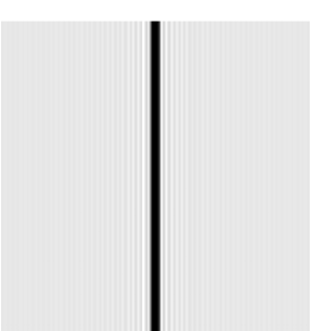
Figure 6: Simulated low and high magnification pictures of an $m=1$, $l=3$ eighth-order sampled graded mask with $\zeta=0$. The low magnification picture (left) shows $\sim 400$ diffraction widths; each stripe has uniform shading and is $f\lambda_{min}$ wide.

5 SUMMARY

We offered a series of eighth-order masks that are relatively insensitive to tip-tilt errors and other low-spatial-frequency aberrations; in a coronagraph using one of these masks, the r.m.s. pointing error only needs to be managed to a few milliarcseconds, no better than the pointing accuracy of the Hubble Space Telescope. Eighth-order notch filter masks retain most benefits of using fourth-order masks—broadband capabilities, reasonably high throughput, and small inner working angle—permitting extremely-high dynamic range coronagraphy suitable for terrestrial planet finding using a popular optical layout.

In particular, we suggested a binary mask designed for TPF-C at 0.5–0.8 $\mu$m composed of opaque strips whose shapes are described by Equation 24 with $m=1$, $l=3$, $\epsilon=0.596$, $N=1.434216871605$, $\hat{M}_{0_{A}}=0.00630889$, $\hat{M}_{0_{B}}=0.01882618$, $C=-0.33935486$, and $\zeta_{0}=0.25941279$. This mask provides 40% Lyot stop throughput and requires an f/115 or slower beam, assuming the mask can be manufactured with an r.m.s. accuracy of 20 nm. The r.m.s. pointing accuracy required for achieving starlight suppression of $10^{-10}$ with this mask in the search area is $\sigma_{\Delta\theta}\approx 4.2$ milliarcseconds for stars of diameter up to $\sim 2.4$ mas. If the mask is used on a telescope with better pointing accuracy, it can achieve contrast levels of $10^{-10}$ on targets with even larger diameters.

We also provided a graded version of this design, whose amplitude transmissivity is described by Equation 24 using the above parameters but with $\zeta=0$. This mask offers the same performance as the above binary version, but it allows easier e-beam fabrication because it only requires optical densities $\leq 7.882$. Other eighth-order masks can provide less ringing at the cost of inner working angle or Lyot stop throughput.

Appendix A APPENDIX

We will prove for a monochromatic coronagraph with a notch filter mask, a binary entrance aperture of finite size, and a Lyot stop that is perfectly opaque everywhere the entrance aperture is opaque, that 1) the PSF shape is the absolute square of the Fourier transform of the Lyot stop amplitude transmissivity independent of the position of the source on the sky, and 2) the PSF is attenuated by the intensity transmissivity of the band-limited part of the mask evaluated at the source position. Kuchner & Traub (2002) demonstrated this principle for a $\sin^{2}$ mask; this more general proof applies to any two-dimensional notch filter mask.

As usual, we will examine a coronagraph comprising an entrance aperture, $A$, an image mask, $\hat{M}$, and a Lyot stop, $L$, each of which is represented by a complex-valued function. We will use the notational conventions of Kuchner & Traub (2002) and Kuchner & Spergel (2003b): letters with hats represent image plane quantities. The image-plane coordinates are ${\bf x}=(x,y)$ and the pupil-plane coordinates are ${\bf u}=(u,v)$.

Monochromatic light propagates through the coronagraph as follows.

• 1) An incoming wave incident on the entrance aperture creates a field with amplitude $E({\bf u})$. When an incoming wave interacts with a stop or mask, the function representing the mask multiplies the wave’s complex amplitude. So after the wave interacts with the entrance aperture, the amplitude becomes $A({\bf u})\cdot E({\bf u})$.

• 2) After the entrance aperture, the beam propagates to an image plane, where the new field amplitude is the Fourier transform of the pupil plane field amplitude, $\hat{A}({\bf x})*\hat{E}({\bf x})$; $*$ denotes convolution. In this plane, the beam interacts with the image mask, and the field amplitude becomes $\hat{M}({\bf x})\cdot(\hat{A}({\bf x})*\hat{E}({\bf x}))$.

• 3) Next, the beam propagates to a second pupil plane, where the field amplitude is $M({\bf u})*(A({\bf u})\cdot E({\bf u}))$. In this second pupil plane, the wave interacts with a Lyot stop, changing the field amplitude to $F({\bf u})=L({\bf u})\cdot[M({\bf u})*(A({\bf u})\cdot E({\bf u}))]$.

• 4) At last, the beam propagates to the final image plane, where the final image field is $\hat{F}({\bf x})$, the Fourier transform of $F({\bf u})$. For a point source, the intensity of the final image is proportional to the absolute value of this quantity squared.

The final image field, $\hat{F}(\bf x)$, and its Fourier transform are linear functions of $A(\bf u)$, $L(\bf u)$, and also $M(\bf u)$. This last property allows us to study masks by decomposing them into Fourier components, computing $F({\bf u})$ or $\hat{F}(\bf x)$ for each one, and then summing the final field amplitudes back together.

Consider a point source providing a field $\hat{E}({\bf x})=\delta({\bf x}-{\bf x_{1}})$ in the plane of the sky and a harmonic mask function $M({\bf u})=\delta({\bf u}-{\bf u_{1}})$. The field after the entrance pupil is $A({\bf u})\exp(-2\pi i\,{\bf u}\cdot{\bf x_{1}})$, and the field in the first image plane is $\hat{A}({\bf x}-{\bf x_{1}})$. The field after the image mask is $\exp(2\pi i\,{\bf u_{1}}\cdot{\bf x})\hat{A}({\bf x}-{\bf x_{1}})$. The field in the second pupil plane is $A({\bf u}-{\bf u_{1}})\exp(-2\pi i({\bf u}-{\bf u_{1}})\cdot{\bf x_{1}})$. The field after the Lyot stop is

$$F({\bf u})=L({\bf u})A({\bf u}-{\bf u_{1}})e^{-2\pi i({\bf u}-{\bf u_{1}})\cdot{\bf x_{1}}}\qquad\mbox{for a harmonic mask.}$$ (A1)

Let $A$ be binary (everywhere equal to 1 or 0) and let $\cal A$ represent the support of $A$ and $\cal L$ represent the support of $L$. If $\cal L\in\cal A$, then there is some set ${\cal P}\in{\cal R}^{2}$ for which $L({\bf u})A({\bf u}-{\bf u_{1}})=L({\bf u})$ for $\bf u_{1}\in{\cal P}$. If $\cal A$ is finite in extent, then there is also some set ${\cal Q}\in{\cal R}^{2}$ for which $L({\bf u})A({\bf u}-{\bf u_{1}})=0$ for $\bf u_{1}\in{\cal Q}$.

Under these circumstances, there are three kinds of harmonic image masks:

• ${\bf u_{1}}\in{\cal P}$: For these harmonic masks, the field after the Lyot stop is uniform in amplitude with a phase gradient ${\bf x_{1}}$.

• ${\bf u_{1}}\in{\cal Q}$: For these masks, the field inside the Lyot stop is zero.

• ${\bf u_{1}}\not\in({\cal P}\cup{\cal Q})$: For these masks, the field after the Lyot stop does not have uniform amplitude.

These three kinds of harmonic masks correspond to the three kinds of virtual pupils illustrated in Figure 6 of Kuchner & Traub (2002).

A band-limited mask is defined to be a continuous sum of harmonic masks of the first variety;

$$\hat{M}({\bf x})=\int_{\bf u_{1}\in P}\,M({\bf u_{1}})\,e^{2\pi i{\bf u_{1}}\cdot{\bf x}}\,d{\bf u_{1}}.$$ (A2)

A notch filter mask is defined to be a continuous sum of harmonic masks of the first and second varieties;

$$\hat{M}({\bf x})=\int_{\bf u_{1}\in(P\cup Q)}\,M({\bf u_{1}})\,e^{2\pi i{\bf u_{1}}\cdot{\bf x}}\,d{\bf u_{1}}.$$ (A3)

Combining this expansion and Equation A1 using the linear property of $F(u)$ described above, we find that in a coronagraph with a notch filter mask, the field amplitude after the Lyot stop is

$$F({\bf u}) = \int_{\bf u_{1}\in(P\cup Q)}\,M({\bf u_{1}})L({\bf u})A({\bf u}-{\bf u_{1}})e^{-2\pi i({\bf u}-{\bf u_{1}})\cdot{\bf x_{1}}}\,d{\bf u_{1}}$$ (A4)

$$= \int_{\bf u_{1}\in P}\,M({\bf u_{1}})L({\bf u})e^{-2\pi i({\bf u}-{\bf u_{1}})\cdot{\bf x_{1}}}\,d{\bf u_{1}}$$ (A5)

$$= L({\bf u})e^{-2\pi i{\bf u}\cdot{\bf x_{1}}}\int_{\bf u_{1}\in P}\,M({\bf u_{1}})e^{2\pi i{\bf u_{1}}\cdot{\bf x_{1}}}\,d{\bf u_{1}}.$$ (A6)

To interpret this equation, let us define the band-limited part of $\hat{M}({\bf x})$ as

$$\hat{M}_{BL}({\bf x})=\int_{\bf u_{1}\in P}\,M({\bf u_{1}})\,e^{2\pi i{\bf u_{1}}\cdot{\bf x}}\,d{\bf u_{1}}.$$ (A8)

Now we can write

$$F({\bf u})=\hat{M}_{BL}({\bf x_{1}})L({\bf u})e^{-2\pi i{\bf u}\cdot{\bf x_{1}}}\qquad\mbox{for a notch filter mask.}$$ (A9)

The final image field is the Fourier transform of this quantity, $\hat{F}({\bf x})=\hat{M}_{BL}({\bf x_{1}})\hat{L}({\bf x-x_{1}})$, and the final image intensity is the absolute square of the Fourier transform of this quantity,

$$|\hat{F}({\bf x})|^{2}=|\hat{M}_{BL}({\bf x_{1}})|^{2}|\hat{L}({\bf x-x_{1}})|^{2}\qquad\mbox{for a notch filter mask.}$$ (A10)

In other words, for a notch filter mask, the PSF shape is $|\hat{L}({\bf x})|^{2}$, independent of ${\bf x_{1}}$, the position of the source on the sky. The PSF is attenuated by a factor $|\hat{M}_{BL}({\bf x_{1}})|^{2}$, the amplitude transmissivity of the band-limited part of the mask evaluated at the source position. The band-limited part of a notch filter mask can generally be found by applying a low-pass filter to the mask function.

References

- Aime et al. (2002) Aime, C., Soummer, R. & Ferrari, A. 2002, A&A, 389, 334
- Burrows et al. (1991) Burrows, C. J., Holtzman, J. A., Faber, S. M., Bely, P. Y., Hasan, H., Lynds, C. R., & Schroeder, D. 1991, ApJ, 369, L21
- Debes et al. (2004) Debes, J. H., Ge, J., Kuchner, M. J. & Rogosky, M. 2004, ApJ, 608, 1095
- Guyon (2003) Guyon, O. 2003, A&A, 404, 379
- Kasdin et al. (2003) Kasdin, N. J., Vanderbei, R. J., Spergel, D. N., & Littman, M. G. 2003, ApJ, 582, 1147
- Kuchner (2005) Kuchner, M. J. 2005, submitted to AJ, (astro-ph/0401256)
- Kuchner & Spergel (2003a) Kuchner, M. J. & Spergel, D. N. 2003a, in Scientific Frontiers in Research on Extrasolar Planets, ASP Conference Series, D. Deming & S. Seager, eds. (astro-ph/0305522)
- Kuchner & Spergel (2003b) Kuchner, M. J. & Spergel, D. N. 2003b, ApJ, 594, 617
- Kuchner & Traub (2002) Kuchner, M. J. & Traub, W. A. 2002, ApJ, 570, 900
- Levine et al. (2003) Levine, B. et al. 2003, Proc. SPIE, 4852, 221
- Shaklan & Green (2005) Shaklan, S. B. and Green. J. J. 2005, to appear in this issue of ApJ
- Traub & Vanderbei (2003) Traub, W. A., Vanderbei, R. J. 2003, ApJ, 599, 695
- Trauger et al. (2004) Trauger, J. et al. 2004, Proc. SPIE, 5487, in press
- Vanderbei et al. (2003a) Vanderbei, R. J., Spergel, D. N., Kasdin, N. J. 2003a, ApJ, 590, 593
- Vanderbei et al. (2003b) Vanderbei, R. J., Spergel, D. N., Kasdin, N. J. 2003b, ApJ, 599, 686