Confronting cosmological simulations with observations of intergalactic metals

Abstract

Using the statistics of pixel optical depths, we compare H I, C IV and C III absorption in a set of six high quality $z\sim 3-4$ quasar absorption spectra to that in spectra drawn from two different state-of-the-art cosmological simulations that include galactic outflows. We find that the simulations predict far too little C IV absorption unless the UVB is extremely soft, and always predict far too small C III/C IV ratios. We note, however, that much of the enriched gas is in a phase ($T\sim 10^{5}-10^{7}\,$K, $\rho/\langle\rho\rangle\sim 0.1-10$, $Z\gtrsim 0.1Z_{\odot}$) that should cool by metal line emission – which was not included in our simulations. When the effect of cooling is modeled, the predicted C IV absorption increases substantially, but the C III/C IV ratios are still far too small because the density of the enriched gas is too low. Finally, we find that the predicted metal distribution is much too inhomogeneous to reproduce the observed probability distribution of C IV absorption. These findings suggest that strong $z\lesssim 6$ winds cannot fully explain the observed enrichment, and that an additional (perhaps higher-$z$) contribution is required.

1. Introduction

Analysis of quasar absorption spectra has revealed that the intergalactic medium (IGM) has been polluted with heavy elements such as carbon, silicon and oxygen (see, e.g., Cowie et al. 1995; Songaila & Cowie 1996; Ellison et al. 2000; Schaye et al. 2003, hereafter S03; Aguirre et al. 2004, hereafter A04; Simcoe et al 2004; Aracil et al. 2004; Boksenberg et al. 2003) At the same time, observations of starburst galaxies (e.g., Shapley et al. 2003) have revealed powerful galactic outflows resulting from feedback processes in galaxies with rapid star formation.

This has led to a picture in which the observed enrichment results from a phase of strong galactic outflows at $z\gtrsim 2$ during the epoch of galaxy formation, and various numerical (e.g., Gnedin 1998; Aguirre et al. 2001; Scannapieco, Ferrara, & Madau 2002; Cen, Nagamine & Ostriker 2004) and semi-analytic (e.g., Furlanetto & Loeb 2003) models have been able to very roughly account for the observed level of metal enrichment. But these comparisons have left many unanswered questions: can, for example, simulations reproduce the detailed density- and redshift-dependent metal distribution? Can they reproduce the abundance ratios of different elements and ions? How is enrichment tied to feedback in galaxies, which is required to suppress runaway star formation?

Recently, both the numerical simulations and observational analyses have improved to the degree that some of these questions can be meaningfully addressed. On the observational side, statistical analyses of pixel optical depths (S03; A04) have inferred the distribution of carbon and silicon using absorption by H I, C IV, C III, Si IV, and Si III (see also Simcoe et al. 2004, who finds consistent results from line fitting of C IV and O VI.) These studies have shown quantitatively that the observed intergalactic carbon enrichment is highly inhomogeneous, density-dependent, nearly redshift-independent, underabundant (relative to silicon), relatively cool ($T<10^{5}\,$K), and persistent at some level even in gas near the cosmic mean density. Meanwhile, hydrodynamic simulations (e.g., Theuns et al. 2002, hereafter T02; Springel & Hernquist 2003a, hereafter SH03) have been produced that probably include all of the galaxies relevant for $z\lesssim 6$ enrichment, use prescriptions for feedback that generate galactic winds, and track metals. SH03 and Hernquist & Springel (2003) have shown in detail that the star formation rate of their simulations has converged, i.e. that the included feedback is sufficient to solve the overcooling problem; T02 have shown that their simulation does not significantly disrupt the Ly$\alpha$ forest, but can roughly account for earlier observations of C IV absorption if the UVB is extremely soft and the yield is $3\times$ solar.

Clearly, it is of interest to carry out detailed comparisons between state-of-the art observations and simulations that include galactic winds. One way to do this is to simply compare the observationally inferred distribution of metals as a function of density and redshift to that predicted by the simulations. This could, however, be misleading. For example, hot, collisionally ionized carbon would be undetectable by observational studies focusing on C IV. A far more direct and robust method is to directly compare simulated and observed absorption spectra. This Letter describes such a comparison. We will draw several qualitatively new conclusions from a comparison of absorption by H I, C IV, and C III in in a set of 6 $z\sim 3$ QSO spectra to that in simulated spectra drawn from the SH03 and T02 simulations.

2. Observations, simulations, and method

We compare our simulations to the observed pixel statistics published in S03 for the redshift range $2.479\leq z\leq 4.033$ (the full sample covers $1.654\leq z\leq 4.451$; we employ a smaller range so that all of the data can be combined without binning in redshift). The data come from six quasar spectra: Q0420-388, Q1425+604, Q2126-158, Q1422+230, Q0055-269, and Q1055+461, that were taken with either the Keck/HIRES or the VLT/UVES instrument. See Table 1 of S03 for information on the sample.

The simulated spectra are drawn from cosmological SPH simulations, using the method described in A02: noise, detector resolution, wavelength coverage, and pixelization are chosen to match the corresponding observed spectra. The ionization balance is computed using CLOUDY, with the same three models for the spectral shape of the UV background (UVB) as we used in S03 and A04: ‘QG’ is a Haardt & Madau (2001) model with contributions from quasars and galaxies; ‘Q’ includes quasars only, and ‘QGS’ is a softened ‘QG’: the flux is reduced by 90% above 4 Ryd. All models are normalized to the H I ionization rate measured by S03, and the simulation metallicities are converted to carbon number densities using the solar abundance $({\rm C/H})_{\odot}=-3.45$ of Anders & Grevesse (1989).

Results are shown for three simulations. The first, ‘NF’, was used and described in A02, S03 and A04: it uses $2\times 256^{3}$ particles in a $12h^{-1}$ Mpc box with $(\Omega_{m},\Omega_{\Lambda},\Omega_{b}h^{2},h,\sigma_{8},n,Y)=(0.3,0.7,0.019,0.65,0.9,1.0,0.24)$. This simulation has no galactic outflows, but for each UVB model we add to the particles the carbon distribution inferred in S03 for that UVB (see Tables 2 and 3 of S03). The second simulation, ‘T’, is described in T02: it uses $2\times 128^{3}$ particles in a $5h^{-1}$ Mpc box with the same cosmological parameters as NF. Here, however, all supernova thermal energy is deposited as feedback, and gas is prevented from cooling for $10^{7}\,$yr (see Kay et. al. 2002) so that strong winds are generated which enrich the IGM. The third simulation, ‘S’, is described in SH03 as their ‘Q4’ model: it uses $2\times 216^{3}$ particles in a $10h^{-1}\,$Mpc box with $(\Omega_{m},\Omega_{\Lambda},\Omega_{b}h^{2},h,\sigma_{8},n,Y)=(0.3,0.7,0.02,0.7,0.9,1.0,0.24)$. It employs both a sub-grid feedback prescription and a wind mechanism in which a velocity of 484 km/s is imparted to certain gas particles in star-forming regions (see Springel & Hernquist 2003b for details). The simulations have approximately the same mass resolution (the baryon particle mass is $\approx 1.1\times 10^{6}{\rm\,M_{\odot}}$ in both), which is adequate to resolve the Ly$\alpha$ forest and to include relatively small galaxies. The use of two simulations allows us to compare the effects of two different feedback prescriptions.

To compare the carbon absorption in simulated and observed spectra, we have employed the pixel optical depth technique described in A02, S03 and A04. This technique (see Cowie & Songaila 1998; Ellison et al. 2000; A02; S03) has several advantages over traditional line-fitting. Perhaps most important here is the ability to measure C III absorption, which is very difficult to do using line fitting because C III is not a multiplet and falls in the Ly$\beta$ forest. Optical depths for H I (Ly$\alpha$), C IV (1548Å), and C III  (977Å)  absorption are extracted from each spectrum for the H I absorption region between the QSO’s Ly$\alpha$ and Ly$\beta$ emission wavelengths, excluding also a small region near the QSO to avoid proximity effects (see S03). The optical depths are corrected for strong contaminating lines, C IV self-contamination by its doublet, and Ly$\alpha$ contamination of C III, as described in A02 and S03.

The pixel optical depths are binned for each QSO and the QSOs are combined as described in A04. In brief, for each QSO the C IV optical depths $\tau_{\rm CIV}$ are binned in H I optical depth $\tau_{\rm HI}$ and the median is taken in each bin. Next, the noise/contamination level, i.e. the median $\tau_{\rm CIV}$ optical depth at very low $\tau_{\rm HI}$, is subtracted from each bin and the ratio $({\rm median}\,\tau_{\rm CIV})/\tau_{\rm HI}$ is computed. Finally, $\tau_{\rm HI}$ bins for different QSOs are combined. The result is a plot of median corrected $\tau_{\rm CIV}/\tau_{\rm HI}$ vs. $\tau_{\rm HI}$, as shown in Fig. 1 (upper left). The same procedure is applied to obtain plots of $\tau_{\rm CIII}/\tau_{\rm CIV}$ vs. $\tau_{\rm CIV}$.

3. Results

Figure 1.— Binned optical depth ratios $({\rm med}\,\tau_{\rm CIV})/\tau_{\rm HI}$ vs. $\tau_{\rm HI}$ (left) and $({\rm med}\,\tau_{\rm CIII})/\tau_{\rm CIV}$ vs. $\tau_{\rm CIV}$ (right) for observations (data points with 1- and 2-$\sigma$ errors) and various models. Top: Models NF-QG (the Q and QGS backgrounds yield similar results), S-QG S-Q, S-QGS, and T-QG, as per the legend. The effect of changing the UVB in the T simulations is similar. Bottom: as in the top panels, but particles with cooling time $t_{c}<t_{H}$ are set to $T=2\times 10^{4}\,$K. The same models are shown, except that the dotted line (‘C1’) corresponds to S-QG if only particles with $t_{c}<0.1t_{H}$ cool (the effect of this change is similar for the other models).

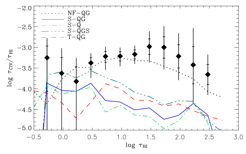
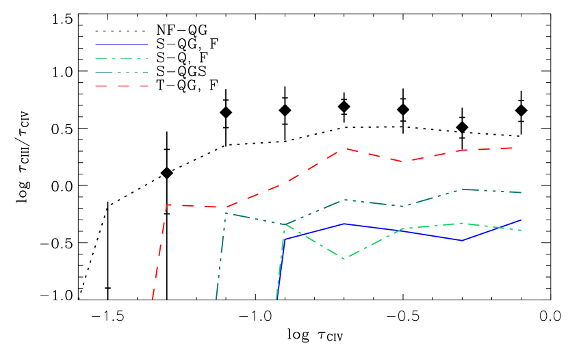
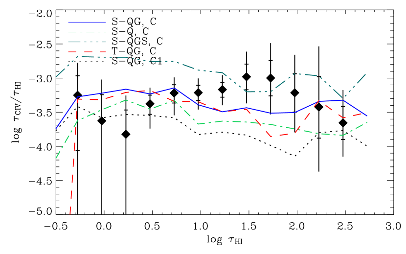
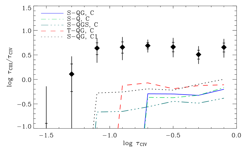
Figure 1 shows median optical depths $({\rm med}\,\tau_{\rm CIV})/\tau_{\rm HI}$ vs. $\tau_{\rm HI}$ (left) and $({\rm med}\,\tau_{\rm CIII})/\tau_{\rm CIV}$ vs. $\tau_{\rm CIV}$ (right) for observations (data points) and three simulations. The dotted line shows the non-feedback (NF) simulation upon which the carbon distribution of S03 has been imposed. The other lines show the SH03 (S) and T02 (T) simulations with the three choices of UVB (QG, Q, and QGS). Except for the extremely soft UVB QGS, the simulations woefully under-predict the median C IV absorption at all $\tau_{\rm HI}$. In Table 1 (column 4) we quantify this by providing the best-fit offset to each set of simulated C IV/H I optical depths (e.g., simulation S-QG is $\approx 1.2\,$dex too low). A super-solar yield could somewhat ameliorate this but seems unlikely for carbon, which is underabundant relative to $\alpha$-elements in the IGM (e.g., A04). Although the QGS models are only 0.26-0.64 dex too low overall, they cannot reproduce the observed shape of $\tau_{\rm CIV}/\tau_{\rm HI}$ vs. $\tau_{\rm HI}$: there is too much absorption at low density (low $\tau_{\rm HI}$) and too little at high-density.

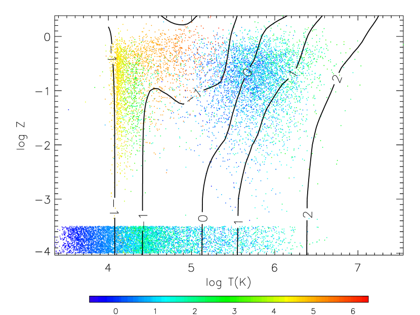
The prime reason for this failure can be seen in Fig. 2, which shows the metallicity, temperature, and density of a random subsample of the S simulation particles (the T simulation is similar). The metal rich intergalactic (overdensity $\log\delta<2$) gas is almost entirely at $T=10^{5}-10^{7}\,$K. Because the C IV/C fraction rapidly falls off at $T\gtrsim 10^{5}\,$K, this gas is essentially invisible in C IV, except at very low density if the UVB is extremely soft.

Even for such an extreme UVB, however, the feedback simulations predict far too little absorption by C III relative to C IV, as can be seen from the upper-right panel of Fig. 1 which shows $({\rm med}\,\tau_{\rm CIII})/\tau_{\rm CIV}$ vs. $\tau_{\rm CIV}$ for the same models. The C III/C IV ratio drops rapidly for $T\gtrsim 10^{5}\,$K and falls roughly linearly with decreasing density for $T\sim 10^{4}\,$K (See Fig. 7 of S03). Thus, the fact that the C IV visible in the feedback simulations is accompanied by insufficient C III means that the enriched gas is too hot and/or of too low density. Note, on the other hand, that the NF simulation reproduces the C III/C IV values quite well once the carbon distribution is chosen to match the C IV/H I values.

The problem that the metals in the feedback simulations are too hot may, however, have a solution. In both simulations the enriched gas is relatively metal-rich by IGM standards ($Z\sim 0.1-1{\,Z_{\odot}}$) and should, in fact, be able to cool via metal line emission, which was not included in the simulations. The contours in Fig. 2 show $\log(t_{c}/t_{H})$, where $t_{c}$ is the radiative cooling time for gas that is in collisional ionization equilibrium computed for overdensity $\delta\equiv\rho/\langle\rho\rangle=1$ ($t_{c}\propto\delta^{-1}$) using Sutherland & Dopita (1993), and $t_{H}$ is the $z=3$ Hubble time. Nearly all of the $\delta\sim 10$ gas and much of the $\delta\sim 1$ gas has $t_{c}<t_{H}$ and should, in the absence of heating, cool to $T\sim 10^{4}\,$K which would increase its visibility in C IV. To test the importance of cooling, we have generated simulated spectra for which all particles with $t_{c}<t_{H}$ are set to $T=2\times 10^{4}\,$K; see bottom panels of Fig. 1. In this case, the QG simulations can roughly match the observed $\tau_{\rm CIV}/\tau_{\rm HI}$ values, although the trend with $\tau_{\rm HI}$ is still not reproduced. The QGS models with cooling now predict too much C IV absorption.

The employed cooling prescription is rather ad hoc. The particle metallicities may be unreliable because the simulation assumes perfect mixing at the particle level and zero mixing between particles once they leave the star forming gas. Furthermore, heating is ignored in the calculation of the cooling times, the gas may not be in collisional ionization equilibrium, conduction is ignored, and the density may not remain constant as the gas cools. To further illustrate the sensitivity of the results to the cooling prescription, the dotted curves in the lower panels of Fig. 1 show the results for the S-QG simulation if the gas cools only when $t_{c}<0.1t_{H}$. The C IV absorption is lower by about 0.5 dex, nearly independent of $\tau_{\rm HI}$. Varying the final temperature between $1-3\times 10^{4}\,$K has a relatively small effect.

Figure 2.— Metallicities (in solar units) and temperatures of particles in the S simulation (only a random 0.5% of metal enriched particles are shown, and 0.05% of the metal-free particles are shown in the scattered bar near $Z=10^{-4}$). The particle colors reflect the log of the gas overdensity as shown by the colored bar: intergalactic $\delta\alt 100$ gas is blue-green; galactic gas (with effective temperatures given by the sub-grid multiphase model) is yellow-red. The contours indicate $\log(t_{c}/t_{H})$ at $\delta=1$ and $z=3$. Since $t_{c}\propto\delta^{-1}$, particles inside the ‘0’ contour at $\delta=1$ can cool, as can particles at $\delta=10$ inside the ‘1’ contour.

Although metal line cooling may help resolve the discrepancy for C IV/H I, it actually makes the problem worse for C III/C IV as can be seen from the bottom right panel of Fig. 1. This indicates that in the simulations the C IV absorption arises in gas with too low a density. The level of $\log\tau_{\rm CIII}/\tau_{\rm CIV}\sim-0.5$ predicted by the simulations indicates that the C IV absorption with $\tau_{\rm CIV}\gtrsim 0.1$ arises in $\delta\sim 1-5$ gas, whereas the corresponding observed absorption appears to occur in gas of $\delta\sim 10-30$ (see Fig. 7 of S03). The increase in density that would very likely accompany the gas cooling may alleviate this problem, but this will have to be determined using future simulations that include metal-line cooling.

Information on the homogeneity of the observed metal distribution can be inferred by using additional percentiles of the $\tau_{\rm CIV}(\tau_{\rm HI})$ distribution (S03). In columns 3–5 of Table 1 we give the best-fit offset to the simulations in the 31st, 50th and 84th percentiles of the C IV distribution. We find that models that can roughly reproduce the medians cannot simultaneously reproduce the other percentiles. In all cases, the metals are too inhomogeneously distributed as compared to the observations (e.g., in S-QG with cooling, the 31st percentile is too low by $\sim 0.8\,$dex while the 84th is too high by $\sim 0.6\,$dex, indicating a wider distribution). This appears to be true independent of the UVB and the cooling prescription and is hence a rather robust inconsistency. It is also interesting because while small-scale unresolved physical effects such as a multiphase structure of the IGM and outflows (or emission from interfaces between phases) are potentially quite important, they seem likely to make the metals appear less rather than more uniformly distributed.

Table 1Comparisons made

Sim-		Offset for percentile in CIV/HI			in CIII/CIV
UVB	Cool	31	50	84	50
NF-QG	-	$0.26\pm 0.13$	$0.15\pm 0.06$	$0.12\pm 0.05$	$0.16\pm 0.05$
S-QG	-	NA	$1.22\pm 0.09$	$0.73\pm 0.07$	$1.00\pm 0.11$
S-Q	-	NA	$1.41\pm 0.10$	$0.73\pm 0.07$	$1.05\pm 0.12$
S-QGS	-	$3.46\pm 0.24$	$0.64\pm 0.06$	$0.41\pm 0.05$	$0.73\pm 0.08$
T-QG	-	NA	$0.94\pm 0.07$	$0.69\pm 0.06$	$0.41\pm 0.07$
T-Q	-	NA	$1.43\pm 0.10$	$0.94\pm 0.07$	$0.58\pm 0.07$
T-QGS	-	$1.40\pm 0.22$	$0.26\pm 0.06$	$0.02\pm 0.05$	$0.56\pm 0.07$t
S-QG	C	$0.82\pm 0.17$	$0.05\pm 0.05$	$-0.59\pm 0.07$	$0.76\pm 0.07$
S-Q	C	$1.14\pm 0.24$	$0.28\pm 0.06$	$-0.16\pm 0.07$	$0.87\pm 0.07$
S-QGS	C	$-0.01\pm 0.13$	$-0.45\pm 0.06$	$-1.42\pm 0.05$	$0.96\pm 0.08$
T-QG	C	$1.18\pm 0.19$	$0.13\pm 0.05$	$-0.31\pm 0.06$	$0.77\pm 0.08$
T-Q	C	$1.29\pm 0.21$	$0.42\pm 0.06$	$0.04\pm 0.06$	$0.68\pm 0.08$
T-QGS	C	$0.10\pm 0.14$	$-0.28\pm 0.06$	$-1.27\pm 0.06$	$1.07\pm 0.12$
S-QG	C1	$2.92\pm 0.20$	$0.48\pm 0.06$	$0.11\pm 0.06$	$0.65\pm 0.06$
S-Q	C1	$3.34\pm 0.27$	$0.63\pm 0.06$	$0.34\pm 0.06$	$0.78\pm 0.07$
S-QGS	C1	$1.60\pm 0.22$	$0.20\pm 0.06$	$-0.46\pm 0.06$	$0.75\pm 0.06$
T-QG	C1	$1.86\pm 0.23$	$0.44\pm 0.06$	$0.18\pm 0.05$	$0.57\pm 0.06$
T-Q	C1	$4.65\pm 0.32$	$0.81\pm 0.07$	$0.47\pm 0.05$	$0.44\pm 0.07$
T-QGS	C1	$0.68\pm 0.18$	$0.09\pm 0.06$	$-0.42\pm 0.06$	$0.84\pm 0.07$

4. Conclusions

A major goal for cosmological simulations is to develop a prescription for feedback with which observations of the IGM and galaxies can be simultaneously reproduced. We have compared in detail the statistics of C IV and C III absorption in a set of six high-quality $z\sim 3-4$ quasar spectra to that in simulated spectra drawn from two tate-of-the-art cosmological SPH simulations with a wide range of UVB models and two different prescriptions for feedback: the simulation of Springel & Hernquist (2003a), which predicts a numerically resolved star formation history that is consistent with the observations and the simulation of Theuns et al. (2002) which matches observations of the H I Ly$\alpha$ forest. We have come to the following conclusions:

• The simulations predict far too little C IV absorption unless the UVB is extremely soft.

• In all cases, the simulations predict far too small C III/C IV ratios.

• The simulations predict that many of the heavy elements reside in gas that is metal-rich ($Z\gtrsim Z_{\odot}$) and hot ($10^{5}\,\lesssim T<10^{7}\,$K). Much of this gas should be able to cool via metal lines, which was not included in the simulations. It will be important to accurately model cooling in future numerical simulations.

• If a crude cooling prescription is applied, the C IV absorption increases significantly, but the predicted C III/C IV ratio is still far too low because the metals reside in gas that is too low density. Cooling should increase the enriched gas density, and this can be estimated in future simulations with metal-line cooling.

• Independent of the cooling prescription, the metal distribution in the simulations is too inhomogeneous to match the observed distribution of $\tau_{\rm CIV}(\tau_{\rm HI})$.

Numerical simulations with strong outflows from $M_{\rm baryon}\gtrsim 10^{8}{\rm\,M_{\odot}}$ galaxies deposit most intergalactic metals in hot, metal-rich bubbles that preferentially inhabit voids and comprise a relatively small filling factor, which allows them to avoid overly disrupting the Ly$\alpha$ forest (Theuns et al. 2002). However, these very attributes appear to prevent them from reproducing the observations of absorption by heavy elements.

If metal cooling is efficient or if the gas has an unresolved multiphase structure then these winds may account for some of the observed enrichment; otherwise they would be largely hidden from current observations. In either case it appears that an additional ingredient – either in the form of another enrichment mechanism, or higher-$z$ enrichment that is unresolved by the simulations – is needed.

References

- Aguirre et al. (2001) Aguirre, A., Hernquist, L., Schaye, J., Weinberg, D. H., Katz, N., & Gardner, J. 2001, ApJ, 560, 599
- Paper (I) Aguirre, A., Schaye, J., & Theuns, T. 2002, ApJ, 576, 1 (A02)
- Aguirre et al. (2004) Aguirre, A., Schaye, J., Kim, T., Theuns, T., Rauch, M., & Sargent, W. L. W. 2004, ApJ, 602, 38 (A04)
- Anders & Grevesse (1989) Anders, E. & Grevesse, N. 1989, Geochim. Cosmochim. Acta, 53, 197
- Aracil, Petitjean, Pichon, & Bergeron (2004) Aracil, B., Petitjean, P., Pichon, C., & Bergeron, J. 2004, A&A, 419, 811
- Boksenberg et al. (2003) Boksenberg, A., Sargent, W.L.W., & Rauch, M. 2003, ApJS, submitted; astro-ph/0307557
- Cen, Nagamine, & Ostriker (2004) Cen, R., Nagamine, K., & Ostriker, J. P. 2004, astro-ph/0407143
- Cowie & Songaila (1998) Cowie, L. L. & Songaila, A. 1998, Nature, 394, 44
- Cowie et al. (1995) Cowie, L. L., Songaila, A., Kim, T., & Hu, E. M. 1995, AJ, 109, 1522
- Ellison et al. (2000) Ellison, S. L., Songaila, A., Schaye, J., & Pettini, M. 2000, AJ, 120, 1175
- Furlanetto & Loeb (2003) Furlanetto, S. R. & Loeb, A. 2003, ApJ, 588, 18
- Gnedin (1998) Gnedin, N. Y. 1998, MNRAS, 294, 407
- Haardt & Madau (2001) Haardt, F. & Madau, P. 2001, astro-ph/0106018
- Hernquist & Springel (2003) Hernquist, L. & Springel, V. 2003, MNRAS, 341, 1253
- Kay, Pearce, Frenk, & Jenkins (2002) Kay, S. T., Pearce, F. R., Frenk, C. S., & Jenkins, A. 2002, MNRAS, 330, 113
- Paper (II) Schaye, J., Aguirre, A., Kim, T., Theuns, T., Rauch, M., & Sargent, W.L.W. 2003, ApJ, 596, 768 (S03)
- Scannapieco, Ferrara, & Madau (2002) Scannapieco, E., Ferrara, A., & Madau, P. 2002, ApJ, 574, 590
- Simcoe, Sargent, & Rauch (2004) Simcoe, R. A., Sargent, W. L. W., & Rauch, M. 2004, ApJ, 606, 92
- Shapley, Steidel, Pettini, & Adelberger (2003) Shapley, A. E., Steidel, C. C., Pettini, M., & Adelberger, K. L. 2003, ApJ, 588, 65
- Songaila & Cowie (1996) Songaila, A. & Cowie, L. L. 1996, AJ, 112, 335
- Springel & Hernquist (2003) Springel, V. & Hernquist, L. 2003a, MNRAS, 339, 312 (SH03)
- Springel & Hernquist (2003) Springel, V. & Hernquist, L. 2003b, MNRAS, 339, 289
- Sutherland & Dopita (1993) Sutherland, R. S. & Dopita, M. A. 1993, ApJS, 88, 253
- Theuns et al. (2002) Theuns, T., Viel, M., Kay, S., Schaye, J., Carswell, R. F., & Tzanavaris, P. 2002, ApJ, 578, L5 (T02)