From gas to galaxies

Abstract

The unsurpassed sensitivity and resolution of the Square Kilometer Array (SKA) will make it possible for the first time to probe the continuum emission of normal star forming galaxies out to the edges of the universe. This opens the possibility for routinely using the radio continuum emission from galaxies for cosmological research as it offers an independent probe of the evolution of the star formation density in the universe. In addition it offers the possibility to detect the first star forming objects and massive black holes.

In deep surveys SKA will be able to detect HI in emission out to redshifts of $z\approx 2.5$ and hence be able to trace the conversion of gas into stars over an era where considerable evolution is taking place. Such surveys will be able to uniquely determine the respective importance of merging and accreting gas flows for galaxy formation over this redshift range (i.e. out to when the universe was only one third its present age). It is obvious that only SKA will able to see literally where and how gas is turned into stars.

These and other aspects of SKA imaging of galaxies will be discussed.

1 Introduction

More and more evidence supports the paradigm that galaxies form hierarchicallly, i.e. that present day galaxies have been built up over cosmological time scales by the coalescence of many smaller, less massive galactic systems [4, 57, 65, 82, 19, 1]. For a particular galaxy this process is described by the so-called merger tree: the accumulation of dark matter mass over time into a final halo. These merger trees are extracted from numerical comological simulations and only describe the merging of dark matter haloes in a robust manner.

Many properties of galaxy populations including current star-formation rates, luminosity functions, the Tully-Fisher relation, morphology segregation, and the variation of star-formation histories with environment are explained by semi-analytical, hierarchical models. However, the role and fate of the gas and stars in this merging process is not well understood due to an incomplete understanding of the relevant physics, the simplicity of the hydrodynamical codes and the lack of numerical resolution. The behaviour of the baryons in these merging dark matter haloes is often described with semi-analytical techniques [53, 7, 19, 20] (see also Baugh et al. (this volume)). In this scheme, the physics of galaxy formation is encoded in a set of rules that are either physically motivated or have been designed to reproduce the results of numerical simulations e.g. the consequences of galaxy mergers. A merger tree (the “family history”) of a dark matter halo is either generated using Monte Carlo techniques or is extracted from an N-body simulation. The uppermost branches of the tree are filled with gas that is shock heated to the virial temperature of these progenitor halos, and a set of rules is followed to describe the subsequent evolution of this gas. Apart from the issue of properly modelling the fate of the baryons, it is also true that the typical shape of a galaxy merger tree has not been confirmed robustly from observations. Observationally, the galaxy mass functions and the merger rates as a function of redshift are largely unknown.

In this picture there still are several key questions that need to be addressed. These are:

• When and how quickly did the gas settle into the dark matter potential wells?

• Where, when and how did the gas get converted into stars?

• When and how did the merging process of small galaxies develop?

• What is the relative importance of gas accretion versus galaxy merging?

• Are galaxies still (trans)forming today?

In order to address these questions it is necessary to have a census of galaxies and their properties over a large range of environments and as large a possible range of cosmic time or redshift. While the stellar content of galaxies can be probed using optical and NIR imaging and spectroscopy using the best facilities on the ground and in space, the only way to probe the cold gas content of galaxies is to use a radio telescope, either at very short wavelengths to measure molecular line emission (see also Blain et al. this volume on molecular lines), or at long wavelengths to measure the HI emission using the 21-cm line. To do this out to redshifts of $z=3$, since when considerable evolution may have taken place [83, 37], requires a radio telescope tenfold larger (in collecting area) than any of the existing facilities. The SKA is such a telescope and the purpose of this chapter is to review the current state of affairs, from both the observational and theoretical points of view, and to outline how the SKA will be instrumental in answering the above questions to which we do not yet have firm answers.

Equally as important, SKA can probe the star formation rates in galaxies using the radio continuum emission. The radio continuum emission provides an estimate of the star formation density with redshift independent of other tracers such as optical or ultraviolet light which is affected by extinction. The caveat is that the relation between the non-thermal radio emission and the star formation rate is assumed not to vary significantly with cosmic time.

The framework for the discussion in this chapter will be the hierarchical structure formation models of Baugh et al. (this volume), who use the technique of semi-analytic modelling to predict the evolution of the HI mass function and the number of star forming radio galaxies, both signposts of evolution to be probed with SKA. This follows a widely accepted idea of how galaxies form, based on the success of the Cold Dark Matter ($\Lambda$CDM) simulations.

Although $\Lambda$CDM has proven to be very succesful in reproducing the WMAP results and resulting large scale structure, SKA will observe the baryonic component of the universe directly. Predictions of what we should observe are still wide open, as recent hydrodynamical simulations indicate that some of the basic assumptions of the semi-analytic models, i.e. that the gas gets heated quickly to the virial temperature, may not be correct. In the semi-analytic modelling the assumption is that the gas gets immediately shock heated to the virial temperature as it flows into the dark matter potential wells. Recently Binney [10], Katz et al. [51] and Murali at al. [66] have pointed out that hydrodynamical simulations suggest that most of the gas is not heated to the virial temperature but accretes slowly in a cool phase from the surrounding large scale structure filaments. The consequence is that galaxies grow through accretion of gas rather than merging of dark matter halos. At redshifts beyond $z\approx 2$ this cool mode of accretion appears to dominate over merging as the main process for galaxy formation. Because these two scenarios differ in the evolutionary scenario of the gas, SKA is the ultimate telescope for distinguishing these from one another.

We will first discuss the properties of radio continuum emission from galaxies and in this context the first luminous objects in the universe. Then we will discuss the subsequent evolution of galaxies following the theoretical scenarios, and finally connect this with the evolution of galaxies which is still ongoing and observable at the present time in the local universe.

2 The radio continuum emission from star–forming galaxies

When and how the first episodes of star formation took place remains a key question of modern cosmology. Much effort has been devoted to measuring the integrated cosmic star formation rate (SFR) of the universe as a function of redshift or look-back time, initially at ultraviolet wavelengths [61], and more recently in the millimetre and radio regimes [12, 38]. Unlike ultraviolet or optical light, radio continuum emission is unaffected by dust, which eliminates the need for uncertain extinction corrections. SKA will detect the radio continuum emission from very large numbers of AGN and star–forming galaxies at redshifts $z>3$. However, we caution that the conversion between a measured radio continuum flux and a derived a global SFR requires the adoption of canonical scaling relations [22] which remain valid out to at least $z\sim$1 [36, 3] but, as we discuss below, may not be directly applicable to primordial star-forming systems at $z>3$.

In the models considered here, the radio continuum emission from star–forming galaxies is computed using the spectro-photometric code GRASIL written by Silva et al.[79]. This code takes star–formation histories generated by GALFORM, including bursts of star formation, and produces a full spectral energy distribution, ranging from the far-UV to the radio. The radio emission includes both synchroton radiation by electrons accelerated in supernova remnants and free–free emission from HII regions. The plots presented in this section are for a model very similar to that of Baugh et al. (this volume). Note that beyond redshifts of $z>6$ inverse compton losses against the cosmic microwave background will begin to affect the synchrotron emission. The non-relativistic, thermal emission is not affected [16] so that radio continuum emission still is a very good tracer of star formation at high redshifts, albeit in another regime.

Figure 1: Predicted 1.4 GHz flux densities for star–forming galaxies (with SFRs of 1, 10 and 100 M_⊙/yr) at different redshifts. The horizontal line at 100 nJy represents the nominal SKA detection limit for an 8 hr integration.

2.1 The first luminous objects (z$>$5)

Little is currently known about the properties of star–forming objects at redshifts above z$\sim 5$ but the next few years are likely to see rapid progress in this area.

Several recent results suggest substantial star formation at high redshift [5]. Studies of the stellar ‘fossil record’ of nearby galaxies for example (e.g. [40]) imply that the star–formation rate in the most massive galaxies increases with redshift and peaks at z=3 or higher. The recent detection of QSOs at redshifts with z$>$6 [28], in which the gas appears to have solar or above-solar metallicity [69] suggests that the massive first stars in the Universe had already formed by z=8 or even earlier. Observations with the HST and ground–based optical/IR telescopes have begun to provide direct measurements of the number of star–forming galaxies at $z\sim$  5–6 [14, 98, 47, 81]. These studies find typical surface densities of $\sim 100$ deg^-2 for star–forming galaxies at $z\sim 6$. So it appears that the global star–formation rate at $z\sim 6$ is roughly similar to that at $z\sim$ 3–4, though with substantial uncertainities because the distribution of high–redshift galaxies appears to be clustered on scales comparable to the diameters of the individual fields studied to date [47].

At even higher redshift, the detections of individual (gravitationally–lensed) galaxies at $z\sim 7$ [58] and $z=10$ [68] have recently been reported, but the density of star–forming galaxies at $z>7$ is essentially unknown at present.

SKA will be a sensitive probe of high-redshift star formation through the detection of radio continuum emission from star–forming regions and the radio afterglows of gamma–ray bursts (GRBs), many of which are now known to arise from the supernova explosions of massive stars.

Models for dwarf galaxies forming in the vicinity of high–redshift QSOs imply likely star–formation rates of 30–60 M$\odot$/yr for these objects [67]. Deep continuum surveys at 1.4 GHz with SKA will reach detection limits of 100 nJy in 8 hr, and as low as 10 nJy in longer integrations of $\sim$1000 hr [86]. This should allow objects with star–formation rates as low as 10 M$\odot$/yr to be detected at redshifts up to z$\sim$4 (8 hr) and z$\sim$11 (in 1000 hr) respectively (see Fig. 1). Individual globular clusters forming at high redshift may also be detectable by SKA, though there are currently few available predictions for the star–formation rates in such objects.

2.2 What will SKA see?

SKA will be able to detect very faint (10–100 nJy) radio continuum sources, i.e. 2–3 orders of magnitude fainter than those seen by present–day telescopes. It is therefore important to keep in mind that simulations of the likely surface density, angular size and redshift distribution of these faint sources require extrapolations from our current knowledge (as well as assumptions about the cosmic evolution of each population). Nevertheless, the work done so far (e.g. [46, 36, 94]) gives us some valuable ideas about what to expect. At 100 nJy, the surface density of continuum sources will be very high ($\sim$200,000 deg^-2), with “normal”, starburst and active galaxies all contributing over a wide range in redshift. Simulations by Hopkins et al. [46] imply that very high–redshift ($z>5$) AGN and starburst galaxies will have surface densities of $\sim$1,000 deg^-2 and $\sim$7,000 deg^-2 respectively in surveys with a detection limit of 100 nJy at 1.4 GHz.

2.3 Distinguishing starbursts from AGN

Although star–forming galaxies dominate the radio source counts at flux densities below about 1 mJy, active galaxies still account for a significant fraction of the population at levels of a few $\mu$ Jy [39]. The problem of distinguishing star–forming galaxies from AGN is discussed by Garrett et al. [35]. Several parameters measurable by the SKA itself (including brightness temperature, morphology, time variability and possibly polarization) can be used, and Garrett et al.[35] show that radio continuum observations with high spatial resolution ($\sim 25$ mas) can reliably distinguish AGN from star forming galaxies at faint flux levels. This would require the SKA to have good sensitivity on baselines of at least 3000 km. High spatial resolution is also required because of the likely source density at flux levels of $\sim$10 nJy, which may be as high as 3 arcsec^-2 [86].

2.4 Probing high–redshift star formation through GRBs

Because of their transient nature, which makes them easy to recognize, and because they appear to be associated with the supernova explosions of young, very massive stars, GRBs may be one of the most direct tracers of star formation at very high redshifts. SKA, with its wide field of view, should be able to detect the radio afterglows of many ‘orphan’ GRB events in which the jet is misaligned with the observer’s line of sight, and thus remains undetected in gamma–rays (e.g. Frail et al [29]). Bromm & Loeb [15] predict that at least 50% of GRBs originate at redshift $z>5$, and Berger et al.[9] find that GRB host galaxies have typical star–formation rates of at least 100 M_⊙/yr. In the next decade, therefore, GRBs are likely to become increasingly common probes of high–redshift star formation up to (and perhaps even within) the epoch of reionization.

2.5 Redshift measurements and estimates

Although SKA will be able to detect many millions of star–forming galaxies over a very wide range in redshift, recognizing the highest–redshift objects will not be straightforward. For most star–forming galaxies with z$<$3, redshifts should be available from the large–area HI surveys which SKA itself will carry out. Alternatives at higher redshift include:
(i) HI absorption lines ([17]; see also Kanekar and Briggs, this volume).
(ii) CO emission–line redshifts, using either the low order transitions observed with SKA, or higher–order transitions observed with ALMA. (see Blain et al. this volume)
(iii) Radio ’photometric redshifts’ based on the spectral slope between 1.4 GHz and 350 GHz [99]. This would require matching high-frequency observations from ALMA.
(iv) Photometric redshift estimates from wide-field multicolour optical/IR images, or spectroscopic measurements in the optical/IR for small samples of particular interest.

3 How different is high–redshift star formation?

In this section, we examine the assumptions underlying the use of the radio continuum to measure SFR, and assess their validity at the high redshifts where SKA will be able to make a unique contribution. We also outline new simulations which will enable us to better interpret the planned deep surveys.

Figure 2: 1.4 GHz radio luminosity (log) plotted against total far–infrared luminosity (taken from Bell 2003 [8]), showing the curvature at low luminosities. Normal star–forming galaxies are plotted as circles, intensely star–forming galaxies as stars (filled stars are ULIRGS, open stars are starbursts). Triangles are BCDs from a comparison sample. The dotted and solid lines represent forward and bisector fits to the data. The thick dashed line shows the trend predicted by the final star–formation calibrations of Bell 2003 [8].

Because of the far-infrared/radio (FIR-R) correlation (e.g. [42]), it is straightforward to show that the radio luminosity in evolved luminous starbursts varies only with SFR [22]. The radio continuum emission below about 10 GHz is dominated by non-thermal emission, which is thought to be proportional to the supernova rate $\nu_{\rm SNR}$. Although the mechanism linking $\nu_{\rm SNR}$ to the non-thermal radio luminosity is complex, depending on poorly understood physics of cosmic-ray confinement and diffusion operating over $10^{7}-10^{8}$ yr, radio continuum surveys have been used to constrain co-moving SFR locally, and at redshifts of up to z$\sim$1–2 [25, 64, 84, 38].

Nevertheless, standard conversion of the radio continuum may not properly estimate the SFR for all galaxies. Low-luminosity dwarf galaxies, particularly BCDs, have higher SFRs than would be estimated by applying canonical relations [56] and also have globally flatter radio spectral indices, clearly reflecting a dominant thermal component [56, 26]. In these galaxies, particularly those of low metal abundance, the SFR derived assuming the standard mix of thermal/non-thermal contributions is underestimated by a factor of five or more [59, 5, 48]. While rare locally (see [60]), low-metallicity low-mass galaxies might be much more frequent at early times and high redshifts, given the predictions of the hierarchical merger models (e.g. Baugh et al. (this volume), [19]. Indeed, such objects may represent the primordial “building blocks” – or “sub-galaxies” [71] – in hierarchical scenarios of galaxy formation. Consequently, at redshifts $z>3$, it is possible that the canonical scaling of SFR with radio continuum does not apply. Such a systematic mis-estimate of SFR could strongly skew our interpretation of deep radio continuum surveys.

3.1 The radio/far-infrared correlation revisited

While the ubiquity of the radio/far-infrared (RFIR) correlation is well documented (e.g. [42, 24, 27, 96, 70, 36, 22, 74], it is also clear that the slope of the relation depends on the characteristics of the sample. Samples dominated by low-luminosity galaxies have steeper than unit slopes [27, 70, 97, 73] but unit or flatter slopes are obtained for high-luminosity samples (e.g. [24, 22, 100]). This is equivalent to saying that the ratio of FIR-to-radio luminosity $q$ ([42]):

$$q=\log\left[\frac{{\rm FIR}/(3.75\times 10^{12}{\rm Hz})}{S_{1.4GHz}}\right]$$

(with FIR = $1.26\times 10^{-14}[\,2.58F_{60\mu{\rm m}}+F_{100\mu{\rm m}}\,]$) increases with decreasing luminosity [8], as shown in Figure 2.

The slope inflection of the FIR-R correlation at low luminosities probably stems from a number of factors involving both the radio continuum and the infrared SED. Moreover, there is some evidence that both the radio continuum and FIR underestimate the SFR at low luminosities [8].

3.2 Luminosity, metallicity, and age: variations in the radio continuum

As noted above, thermal emission increasingly dominates the radio spectrum of galaxies with low luminosity and low metallicity in general, and this is reflected in their flatter radio spectral indices [56, 55, 26]. The same trend is seen in galaxies with very young star-forming regions, where non-thermal radio emission is virtually absent [72]. The SFR estimated by assuming a purely thermal spectrum is roughly ten times higher than inferred from a “standard” mainly non-thermal spectrum [22].

Moreover, optically thick HII regions are very likely to be prevalent in young starbursts [59, 5, 6]. This means that instead of a flat thermal spectrum, we would see a rising or highly-absorbed spectrum at $\sim$ 1 GHz, which would again alter the standard assumptions. Such an effect would also be expected to vary with redshift.

Figure 3: The integrated star–formation history of the Universe, from [40]. The SFR calculated from the “fossil record” in the Sloan Digital Sky Survey (SDSS) is shown by the eight large filled circles. The other symbols correspond to independent determinations using instantaneous measurements of the star formation rate at various wavelengths.

Figure 4: Local ($z<0.1$) star–formation density for galaxies with star–formation rates between 0.01 and 1000 M_⊙ yr^-1 [73]. The solid line is derived from a fit to the local radio luminosity function for star–forming galaxies, while filled squares show values derived from optical measurements of the H$\alpha$ emission line [34]. In the local universe, the most likely place for a star to form appears to be in a galaxy with a star–formation rate around 10 M_⊙  yr^-1. The integral under this plot is the zero-point of the ’Madau diagram’ which plots the integrated star–formation density at different redshifts.

If non-thermal radio emission is suppressed in low-luminosity galaxies, the disk magnetic field must either be absent or substantially weaker than in galaxies with higher luminosities (see [56, 55, 73]). If the starbursts are young, it could also mean that there has not been enough time to set up the usual $10^{8}$ yr diffusion of cosmic ray electrons [41]. If the radio emission is also compact ($<$200 pc), such as that in many BCDs (e.g., SBS 0335$-$052), there can be no $\sim$kpc large-scale diffusion. This means that any non-thermal emission must be produced by a different mechanism (e.g. evolved supernovae expanding in a dense medium [18, 2]; young supernova remnants; etc.).

In any case, the inescapable implication of the radio spectral differences as a function of luminosity, metallicity, or age is that the conversion of radio continuum to SFR may change as a function of redshift. While this is probably not an issue with current facility surveys which probe only a limited redshift regime, deep SKA surveys will be able to detect not only the most luminous radio sources at each redshift, but also adequately sample the statistically dominant “normal” star-forming population out to redshifts of 10 or so. Changes in the conversion factors as a function of redshift need to be considered when mapping cosmic star formation.

3.3 The evolving stellar content of galaxies

The integrated star-formation history of the universe (the Madau diagram; see Fig. 3) is likely to be accurately mapped out fairly soon. This tells us how much star–formation occurred at a given cosmic epoch, but to understand galaxy evolution we need to know more than this. In particular, where and in what range of environments, did star formation occur at each epoch? Did most stars form in galaxies undergoing “quiescent”star formation, or in galaxies undergoing violent starbursts, and how does this vary with redshift? How important a role do mergers play in triggering star formation? In the local universe, star formation occurs in a wide range of environments, and in galaxies with star–formation rates ranging over at least five orders of magnitude (Fig. 4). There is no reason to suppose that the high–redshift universe is any less diverse.

Understanding the evolving stellar content of galaxies, and the chemical enrichment of the interstellar and intergalactic medium which accompanies this, requires a multi-wavelength approach. ALMA is sure to have a big impact, and will be a powerful tracer of star–forming galaxies over a wide redshift range, detecting large numbers of normal star–forming galaxies out to z$\sim$3 and Arp 220–like starbursts to z$\sim$10 (e.g. [95]). But SKA can equally well chart out such luminous star burst galaxies at almost any redshift and has the great advantage of a much larger field of view and hence superior survey capabilities. Moreover, unlike ALMA, the sensitivity of SKA to star formation does not depend on the presence of metals. Since the first stars must form in a primordial metal-free environment, molecular clouds would not be expected to contain CO or other molecules beyond molecular hydrogen. Hence SKA will provide a much ”cleaner” less biased view of high-redshift star formation.

4 The assembly of galaxies ($0.2<z<5$).

SKA has the unique ability to trace the transformation of HI gas into stars (and into the enriched hot gas which future X–ray missions will detect) in a wide range of environments and over a large fraction of cosmic time. The fact that HI observations trace the depth of a galaxy’s potential, and so can relate star–formation to halo mass as well as to luminosity, is also important because it allows direct tests of galaxy evolution models which deal with mass as well as light.

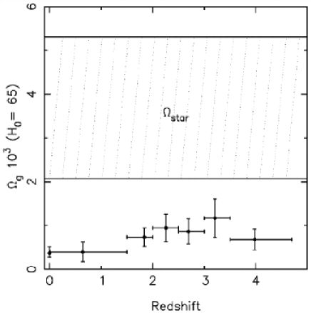
Figure 5: Comoving HI mass density in neutral gas contributed by damped Ly$\alpha$ absorbers plotted as a function of redshift for a cosmology with $\Omega_{M}$ = 0.27, and $\Omega_{\Lambda}$ = 0.73  [83]. The region $\Omega_{\rm star}$ is the $\pm 1\sigma$ range for the mass density in stars in nearby galaxies [33]. The point at z = 0 is the value inferred from 21 cm emission from local galaxies [103].

Figure 6: The evolution of the HI mass function with redshift in the Baugh et al. (this volume) model. The points show the recent determination using HIPASS galaxies by Zwaan et al.[106]. The curves show the model predictions at different redshifts (solid: z=0 ; dotted: z=1 ; dashed: z=3, dot-dashed: z=4).

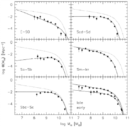
Figure 7: The HI mass function for different morphological types. Shown are Schechter fits (solid lines) and the overall HI mass function for the total sample (dashed line). From Zwaan et al.[106].

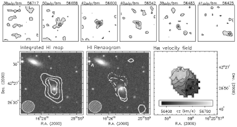
Figure 8: Atomic Hydrogen detected in Abell 2192 at z=0.1887. Upper panels: individual channel maps from the VLA datacube. The rms noise and Heliocentric velocity are noted above each panel. Lower left: Total HI map. The contours coincide with the position of an inclined barred late-type galaxy. Lower middle: contours from the three channel maps plotted on top of each other; solid: cz=56483 km/s, dashed: cz=56542 kms, dotted: cz=56600 km/s. Lower right: H$\alpha$ velocity field of the optical counterpart obtained with the PMAS IFU spectrograph at the 3.5m telescope on Calar Alto. There is excellent correspondence between the HI and H$\alpha$ recession velocities, confirming the HI detection. From Verheijen and Dwarakanath (in preparation).

4.1 basic SKA capabilities for HI emission observations

Before discussing how SKA will contribute to probing the gas content of the universe over cosmic time we will briefly describe its capabilities in terms of sensitivity and resolution to provide a baseline for HI imaging projects. HI line observations typically require a brightness sensitivity of a few Kelvin, which in practice limits the angular resolution. For SKA this implies the following: if one takes as a guideline a $T_{b}$ sensitivity of $\sim 1$ Kelvin in a $0.5^{\prime\prime}$ beam at 1.4 GHz (so baselines out to at most a few hundred km), then one can detect $L_{*}$ galaxies out to a redshift of $z=1.5$ in a 12 hour integration. Although the current design goals require a field of view of one square degree at 1.4 GHz, a much wider field of view appears technically feasible, and would provide an impressive gain in survey speed (see also Blake et al. this volume).

Table 1 gives an indication of the 5$\sigma$ HI detection limits for a 12 hour integration assuming a velocity width of 100 km sec^-1. The calculations assume H₀ = 71 km sec^-1 Mpc^-1, $\Omega_{M}$ = 0.27, and $\Omega_{\Lambda}$ = 0.73. The calculations followed the SKA strawman design figures: A_rme/T_sys = 20000, 70% of the collecting area is within 100 km and assumed two polarizations.

Table 1: Detection limits for HI emission with SKA ⁽¹⁾

$z$	Freq.	Tsys (2)	Angular (3)	Linear	SB	Luminosity	Lookback	HI mass (4)
			Resol.	Resol.	Dimming	Distance	Time	limit
	(MHz)	(K)	(arcsec)	(kpc)	(mag)	(Gpc)	(Gyr)	(M⊙)
0.2	1183.67	50.4	0.52	1.7	0.796	0.972	2.41	$6.1\times 10^{8}$
0.5	946.94	51.4	0.65	4.0	1.486	2.825	5.02	$8.7\times 10^{8}$
1.0	710.20	53.8	0.87	7.0	3.026	6.640	7.73	$2.7\times 10^{9}$
1.5	568.16	57.5	1.09	9.3	4.000	11.02	9.32	$7.2\times 10^{9}$
2.0	473.47	62.7	1.31	11.1	4.796	15.75	10.32	$1.5\times 10^{10}$
2.5	405.83	69.6	1.52	12.5	5.469	20.72	11.00	$2.6\times 10^{10}$
3.0	355.10	78.3	1.74	13.6	6.052	25.87	11.48	$4.3\times 10^{10}$
3.5	315.64	89.3	1.96	14.6	6.566	31.15	11.83	$6.7\times 10^{10}$

¹  assuming t = 12 hours, A_e/T_sys=20000, 2 polarizations and 70% of A_e within 100 km)
  ²  including a contribution from Galactic foreground emission assuming T${}_{\rm Gal}(f_{\rm MHz})$ = 20$(\frac{408}{f_{\rm MHz}})^{2.7}$ K
  ³  fixed array geometry assumed so that resolution scales with wavelength
  ⁴  assuming 5 rms and 100 km sec^-1 profile width. At z=0.2 and z=0.5 the galaxies are assumed resolved      so here the flux has been added over 8.5 and 1.5 beams respectively.

It is clear from Table 1 that it is possible to detect large galaxies in HI emission beyond a redshift of $z=1$ fairly easily, though with limited resolution. For example a galaxy like the Milky Way can be detected out to a redshift of about 1 in a 12 hour integration. Its companions, the Magellanic Clouds, can still be seen out to redshifts of a few tenth. Large spiral galaxies such as M 101 can be probed much farther, to $z\approx 2.5$.

4.2 The evolving gas content of galaxies

Various lines of evidence suggest that there is strong evolution between $z=1$ and $z=3$. This is shown not only by the latest estimates of the change in comoving star formation density with redshift [40] but also by the most recent estimates of the evolution in gas density with redshift from damped Ly$\alpha$ studies [83, 37].

Direct measurements of the evolution of the HI in galaxies out to redshifts of 1 and beyond are not yet available, because present day instruments lack the sensitivity and resolution to directly measure the HI in galaxies at these redshifts. The largest redshift HI detection to date is a deep VLA observation of the cluster Abell 2192 at $z=0.1887$ [92] which detected HI in a late type galaxy at this redshift (see Fig. 8 ). Scaling this observation to the capabilities of SKA one expects to get similar results for galaxies at distances beyond $z=1$.

Damped Ly$\alpha$ studies  [83] indicate that the comoving HI mass density is a few times the present value beyond $z=1$ and out to $z=3$ as illustrated in Fig. 5. The evolution in comoving HI mass density as shown in Fig. 5 is still dependent on assumptions. A recent study of the column density distribution function of HI from observations of nearby galaxies by Zwaan et al.  [106] suggests that there is not as strong an evolution in comoving HI mass density as suggested in Fig. 5. SKA, however, will be able to measure the HI emission in galaxies back to redshifts of $z\approx 3$ directly and will revolutionize this area of research.

There are various ways in which the SKA will contribute significantly to determining the way in which galaxies assemble over cosmic time. Since the evolution of comoving HI gas density as described above has not been directly measured, but has been derived from HI column density measurements of Damped Ly$\alpha$ absorbers it is crucial to be able to image the entire HI disks associated with these Damped Ly$\alpha$ absorbers. If the associated HI masses are indeed of the order of M${}^{*}_{\rm H\kern 0.70004pt{\scriptsize I}~{}}$ = $6.2\times 10^{9}$ M_⊙ [104, 105, 106] then SKA can image these disks out to $z=1.4$ in integration times of 12 hours. Such observations will be crucial for linking the existing column density measurements to the local HI density from observations of the emission.

Another way to probe the evolution of galaxies over cosmic time is to determine variations in the HI Mass Function as a function of environment (local galaxy density) and redshift. From recent studies (see Fig. 7 from Zwaan et al. [106]) it is already apparent that the HI mass function depends on Hubble type. The HI mass function also appears to depend on environment. The slope of the overall HI mass funtion is steeper ($\sim-1.3$ [106]) than in the Local Group [107] and Ursa Major cluster [93] where the slope is $\sim-1.0$. So by measuring the HI mass function over a range of redshifts and in different environments one can probe the effects of galaxy evolution. The models of Baugh et al. (this volume) also indicate changes in the HI mass function (see Fig. 6) which SKA will be able to determine.

In order to do this reliably, sufficient numbers of galaxies over a range of HI masses need to be detectable. A deep HI survey using of order 30 days of integration time will be able to detect L_∗ galaxies (which typically have HI masses of $6.2\times 10^{9}$ M_⊙ assuming H₀ = 71 km/s/Mpc) out to redshifts of $z\approx 2.7$, i.e. beyond the redshift where the universe shows considerable evolution. Using the HI mass function of Zwaan et al.(2003) [105] and assuming no evolution of the HI properties of galaxies with redshift one can calculate how many galaxies one would expect to detect per redshift interval in a one square degree field of view. Table 2 gives a brief summary. These calculations were performed for a $\Omega_{M}=0.27$ and $\Omega_{\Lambda}=0.73$ cosmology. In such long integrations the emission associated with Damped Ly$\alpha$ systems in the field of view can be detected out to $z\approx 2.7$ (assuming they are $\approx$ M${}^{*}_{\rm{HI}}$ systems).

Table 2: Detectable HI Masses as a function of redshift and number of detected galaxies per
square degree in 360 hour and 1000 hour integrations

Redshift	Look Back Time	HI Mass Limit (1)	Number	HI mass limit (1)	Number
	(Gyr)	( M⊙)	of detections	( M⊙)	of detections
		t = 360 h		t = 1000 h
0.5 – 1.0	5.0 – 7.7	$5.0\times 10^{8}$	$1.6\times 10^{6}$	$3.0\times 10^{8}$	$2.4\times 10^{6}$
1.0 – 1.5	7.7 – 9.3	$1.3\times 10^{9}$	$1.8\times 10^{6}$	$7.9\times 10^{8}$	$2.7\times 10^{6}$
1.5 – 2.0	9.3 – 10.3	$2.7\times 10^{9}$	$1.9\times 10^{6}$	$1.6\times 10^{9}$	$2.7\times 10^{6}$
2.0 – 2.5	10.3 – 11.0	$4.8\times 10^{9}$	$1.7\times 10^{6}$	$2.9\times 10^{9}$	$2.5\times 10^{6}$
2.5 – 3.0	11.0 – 11.5	$7.8\times 10^{9}$	$1.6\times 10^{6}$	$4.7\times 10^{9}$	$2.3\times 10^{6}$
3.0 – 3.5	11.5 – 11.8	$1.2\times 10^{10}$	$1.4\times 10^{6}$	$7.3\times 10^{9}$	$2.0\times 10^{6}$
3.5 – 4.0	11.8 – 12.1	$1.8\times 10^{10}$	$1.2\times 10^{6}$	$1.1\times 10^{10}$	$1.8\times 10^{6}$
4.0 – 4.5	12.1 – 12.3	$2.7\times 10^{10}$	$1.0\times 10^{6}$	$1.6\times 10^{10}$	$1.5\times 10^{6}$

¹  calculated for the larger $z$ in each interval. Other assumtions as in table 1.

Out to $z\approx 0.3$ one will be able to resolve a fair fraction of the galaxies so one can obtain rotation curves, mass distributions, and gas fractions for more than $\approx 10^{4}$ galaxies between now and 3 Gyr ago. One then is in a unique position to trace the evolution of the ISM in galaxies over a substantial fraction of the age of the universe, from the era of strongest evolution and star formation activity until the present. In addition one would learn whether and how the evolution depends on the dark matter content and environment.

The hierarchical galaxy formation simulations suggest that most of the evolution in the HI mass function is in the mass range M${}_{H\kern 0.70004pt{\scriptsize I}~{}}$ = 4 $\times$ 10⁸ – 4 $\times$ 10⁹ M_⊙and within the last seven billion years. Fig. 6 shows that at $z=1$ one expects $\sim 3$ times more galaxies in this mass range than at $z=0$. This figure also illustrates that there is very little evolution in the high mass ( M${}_{\rm{H\kern 0.70004pt{\scriptsize I}~{}}}$ $>4\times$ 10⁹ M_⊙) end of the HI mass function. This is the range where the SKA is especially sensitive and can probe easily to at least $z=1$, so that this prediction can be verified.

If, on the other hand, the suggestion that the gas accretes along filaments and is not heated to the virial temperature  [10, 51, 66] is correct, then a deep SKA survey should be able to see the filamentary cool gas reservoirs out to $z=3$ since until $z\approx 1$ there is as much gas in filaments as there is in galaxies. Since in this picture the size of the filaments that feed the galaxies grow from galaxy size at high redshift, to hundreds of kpc size structures feeding entire groups at low redshifts, deep HI surveys should be able to verify this idea. If on the other hand mergers of predominantly small systems are the main process one expects to find a very different distribution of HI structures with redshift.

In addition, as detailed in the previous section, one can use the continuum emission to probe the star formation rates of the detected galaxies, independent of the effects of extinction using the radio continuum-FIR correlation  [42, 41, 21, 22, 78] and test the model predictions. In addition, this information can be used to link the star formation rates to the HI contents of galaxies as a function of redshift and environment. The global star formation rates can be compared with the semi-analytic models and the cool gas accretion models in order to test the predictions. That environment plays an important role is suggested by the analysis of Sloan Digital Sky Survey (SDSS) data [53, 52, 45, 44] which shows a dependence of galaxy mass and star formation rate on environment.

5 Evolution now ($z<0.2$).

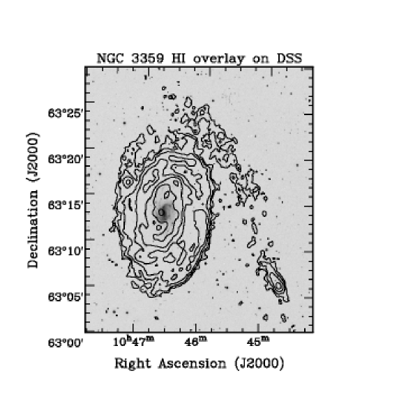
Figure 9: HI distribution of NGC 3359 at a resolution of 30^′′ superposed on the digital sky survey image (left panel). Contours are 0.1, 0.2, 0.4, 0.8, 1.6, 3.0, and 5.0 $\times 10^{21}$ cm^-2 [87]

The process of merging and accretion continues to the present time. Ample evidence is already provided from existing observations, both optical and HI imaging. Zaritsky [101] and Zaritsky & Rix [102] studied several tens of galaxies and ascribed the coincidence of evidence for recent star formation from stellar population studies with measurable asymmetries in the galaxy shapes, to recent accretion events. Kinematic lopsidedness, observed in the 2 dimensional HI velocity fields of galaxies [90, 85] has also been considered as a result of recent minor mergers. Furthermore there are at least twenty examples of galaxies which in HI show either signs of interactions and/or have small companions [75, 76, 87]. This suggests that galaxies often reside in an environment where material for accretion is available. An example is given in Fig. 9 which shows a new HI image of the galaxy NGC 3359 which is accreting gas from a faint HI companion.

Other clear evidence for ongoing minor merger activity comes from the discovery of the Sagittarius dwarf galaxy [49] and of substructure in the halo of the Local Group galaxy M 31 [50, 23, 63].

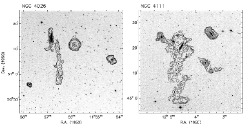
Figure 10: Extended HI filaments observed near the brightest lenticular galaxies in the Ursa Major cluster. These lenticulars are located in small sub-groups within the Ursa Major volume. and the HI morphology indicates that tidal interaction between the galaxies is taking place. From Verheijen and Zwaan [91]

The HI Rogues Gallery of Galaxies [43],  www.nrao.edu/astrores/HIrogues/) gives a glimpse of the role of gas in galaxy evolution at $z=0$. Ideally one would want to make complementary Rogues Galleries at $z=0.5$, $z=1$, $z=1.5$, and $z=2$ to study the process of accretion in detail. Inspection of the Rogues Gallery clearly demonstrates the importance of using the HI for probing galaxy evolution. The prospect of obtaining similar information to either higher depth in sensitivity or to much larger redshifts is truly exciting as radio observations are the only means to probe these aspects of galaxy evolution. There simply is no other way to trace the neutral atomic gas around galaxies. A very good illustration is the extended HI around SO galaxies in the Ursa Major cluster shown in Fig. 10. SO galaxies are thought to be the result of galaxy transformation by gas removal (stripping and/or tidal effects) but in these objects this is not so obvious. A second example of the diagnostic power of HI imaging is NGC 4522 in the Virgo cluster, where the HI morphology presents overwhelming evidence that stripping by ram pressure is taking place. (see Fig. 11)

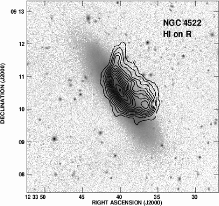
Figure 11: NGC 4522 in the Virgo cluster from Kenney et al. [54]. The HI contours are displaced from the optical disk and clearly show the sweeping effect of ram-pressure stripping.

That indeed the environment plays an important role in determining the HI properties (and hence probably the evolution) of galaxies has become clear from different lines of evidence (for a recent review see van Gorkom [89]): the finding that galaxies in clusters out to 2 Abell radii are deficient in HI as compared to galaxies of similar type in the field [80], see also Fig. 12 ) and the truncated and sometimes displaced HI distributions of galaxies in rich environments (resulting from ram pressure stripping and tidal effects). Additional evidence for strong environmental effects is shown in Fig. 13 from Verheijen et al.  [91]. In the denser environments of the core of the Virgo cluster the HI deficiencies and HI to optical sizes are notably different (respectively larger and smaller) than in the less dense environment of the Ursa Major cluster and the field.

The velocity structure and spatial distribution of HI detected galaxies near clusters suggests that infall is still going on and that clusters are still capturing galaxies which fall in along large scale structure filaments. Evidence such as the HI structures around S0 galaxies and the stripped gas in NGC 4522 (Fig. 10 and Fig. 11) are crucial in pinning down these processes and SKA will be able to see such structure over a considerable range of redshift (i.e. evolution).

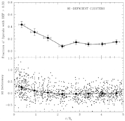
Figure 12: Top: HI deficient fraction in bins of projected radius from the cluster center for the superposition of all the HI deficient clusters. Bottom: HI deficiency versus projected radius from the cluster center. Small dots show the radial variation of HI deficiency for individual galaxies, while the arrows indentify non detections plotted at their estimated lower limit. Large dots are the medians of the binned number distribution. From Solanes et al. [80].

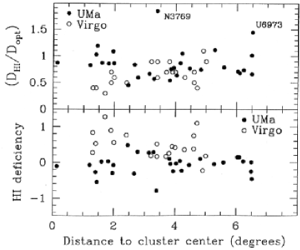
Figure 13: A comparison of HI properties of galaxies in the Ursa Major and Virgo clusters as a function of projected distance to the cluster center. Upper panel: ratio of HI to optical diameters. Lower panel: overall HI deficiency as a function projected distance.

A shallow survey covering 100 square degrees in two months (assuming 100 km sec^-1 profile width, a 5$\sigma$ detection limit, a field of view of one square degree at 1.4 GHz , and an instantaneous bandwidth of 500 MHz) will be able to see NGC 3359–like structures to $z=0.15$ opening the exciting prospect of being able to probe the environment of several million galaxies and pin down the merger/accretion characteristics at the present time over a range of galaxy densities. The resolution and sensitivity of such a survey will be comparable to that of the images shown in Fig. 9 and Fig. 10. The volume covered by such a survey is $\sim$ 15,000 Mpc³ and will detect $\sim$ half a million galaxies, providing a detailed HI image, not only of the galaxies but also of their HI environments. Only with such data can the evolution of galaxies, in particular the mechanisms for converting gas into stars in and around galaxies be studied.

References

- [1] Abadi M.G., Navarro J.F., Steinmetz M., Eke V.R., 2003, ApJ, 591, 499
- [2] Allen, M. L. & Kronberg, P. P. 1998, ApJ, 502, 218
- [3] Appleton, P.N., Fadda, D.T., Marleau, F.R., Frayer, D.T., Helou, G., Condon, J.J., Choi, P.I., Tan, L., Lacy, M., Wilson, G., Armus, L., Chapman, S.C., Fang, F., Heinrichson,I., Im, M., Januzzi, .T., Storrie-Lombardi, L.J., Shupe, D., Soifer, B.T., Squires, G. & Teplitz, H.I., 2004, astro-ph/0406030
- [4] Baugh C.M., Cole S., Frenk C.S., 1996, MNRAS, 283, 1361
- [5] Beck, S. C., Turner, J. L., & Kovo, O. 2000, AJ, 120, 244
- [6] Beck, S. C., Turner, J. L., Langland-Shula, L. E., Meier, D. S., Crosthwaite, L. P., & Gorjian, V. 2002, AJ, 124, 2516
- [7] Benson, A. J., Pearce, F. R., Frenk, C. S., Baugh, C. M., & Jenkins, A. 2001, MNRAS, 320, 261
- [8] Bell, E. F. 2003, ApJ, 586, 794
- [9] Berger, E., Cowie, L.L., Kulkarni, S., Frain, D.A., Aussel, H, Barger, A.J., 2003, ApJ, 588, 99
- [10] Binney, J. 2004, MNRAS, 347, 1093
- [11] Blain, A. W., Barnard, V. E., & Chapman, S. C. 2003, MNRAS, 338, 733
- [12] Blain, A. W., Smail, I., Ivison, R. J., & Kneib, J.-P. 1999, MNRAS, 302, 632
- [13] Boomsma, R., Oosterloo, T., van der Hulst, J. M., & Sancisi, R. 2003, IAU Symposium, 217, ASP Conf. Ser., in press
- [14] Bouwens, R.J. et al. 2003, ApJ, 595, 589
- [15] Bromm, V., Loeb, A. 2002, ApJ, 575, 111
- [16] Carilli, C. L. & Yun, M. S. 1999, ApJ, 513, L13
- [17] Carilli, C.L., Gnedin, N.Y., Owen, F. 2002, ApJ, 577, 22
- [18] Chevalier, R. A. & Fransson, C. 2001, ApJl, 558, L27
- [19] Cole, S., Lacey C.G., Baugh, C.M. & Frenk, C.S., 2000, MNRAS319, 186
- [20] Cole, S., Aragon-Salamanca, A., Frenk, C. S., Navarro, J. F., & Zepf, S. E. 1994, MNRAS, 271, 781
- [21] Condon, J. J., Anderson, M. L., & Helou, G. 1991, ApJ, 376, 95
- [22] Condon, J. J. 1992, ARA&A, 30, 575
- [23] Ferguson, A. M. N., Irwin, M. J., Ibata, R. A., Lewis, G. F., & Tanvir, N. R. 2002, AJ, 124, 1452
- [24] Cox, M. J., Eales, S. A. E., Alexander, P., & Fitt, A. J. 1988, MNRAS, 235, 1227
- [25] Cram, L., Hopkins, A., Mobasher, B., & Rowan-Robinson, M. 1998, ApJ, 507, 155
- [26] Deeg, H., Brinks, E., Duric, N., Klein, U., & Skillman, E. 1993, ApJ, 410, 626
- [27] Devereux, N. A. & Eales, S. A. 1989, ApJ, 340, 708
- [28] Fan, X., et al. 2003, AJ, 125, 1649
- [29] Frail, D.A. et al. 2001, ApJ, 562, L55
- [30] Fraternali, F., Oosterloo, T., & Sancisi, R. 2004, Ap&SS, 289, 377
- [31] Fraternali, F., van Moorsel, G., Sancisi, R., & Oosterloo, T. 2002, AJ, 123, 3124
- [32] Fraternali, F., Oosterloo, T. A., Sancisi, R., van Moorsel, G., & Cappi, M. 2002, ASP Conf. Ser. 276: Seeing Through the Dust: The Detection of HI and the Exploration of the ISM in Galaxies, 419
- [33] Fukugita, M., Hogan, C. J. & Peebles, P. J. E. 1998, ApJ, 503, 518
- [34] Gallego, J., Zamorano, J., Aragon-Salamanca, A., & Rego, M. 1995, ApJ, 455, L1
- [35] Garrett, M.A. et al. 2001, A&A, 366, L5
- [36] Garrett, M.A., 2002, A&A, 384, L19
- [37] Giavalisco, M., et al. 2004, ApJ, 600, L103
- [38] Haarsma, D. B., Partridge, R. B., Windhorst, R. A., & Richards, E. A. 2000, ApJ, 544, 641
- [39] Hammer, F., Crampton, D., Lilly, S.J., Le Fevre, O., Kenet, T. 1995, MNRAS, 276, 1085
- [40] Heavens, A., Panter, B., Jimenez, R., Dunlop, J. 2004, Nature, 428, 6983
- [41] Helou, G. 1991, ASP Conf. Ser. 18: The Interpretation of Modern Synthesis Observations of Spiral Galaxies, 125
- [42] Helou, G., Soifer, B. T., & Rowan-Robinson, M. 1985, ApJ, 298, L7
- [43] Hibbard, J. E., van Gorkom, J. H., Rupen, M. P., & Schiminovich, D. 2001, ASP Conf. Ser. 240: Gas and Galaxy Evolution, 657
- [44] Hogg, D. W., et al. 2004, ApJ, 601, L29
- [45] Hopkins, A. M., et al. 2003, ApJ, 599, 971
- [46] Hopkins, A., Windhorst, R., Cram, L., Ekers, R. 2000, Experimental Astronomy, 10, 419
- [47] Hu, E.M., Cowie, L.L., Capak, P., McMahon, R.G., Hayashino, T., Komiyama, Y. 2004, AJ, 127, 563.
- [48] Hunt, L. K., Dyer, K. D., Thuan, T. X., & Ulvestad, J. S. 2003, ApJ, submitted
- [49] Ibata, R., Irwin, M., Lewis, G., Ferguson, A. M. N., & Tanvir, N. 2001, Nature, 412, 49
- [50] Ibata, R. A., Gilmore, G., & Irwin, M. J. 1994, Nature, 370, 194
- [51] Katz, N., Keres, D., Dave, R., & Weinberg, D. H. 2003, Astrophysics and Space Science Library Vol. 281: The IGM/Galaxy Connection. The Distribution of Baryons at z=0, 185
- [52] Kauffmann, G., White, S.D.M., Heckman, T.M., Menard, B., Brinchmann, J., Charlot, S., Tremonti, C. & Brinkmann, J. 2004, MNRASsubmitted, Astroph/0402030
- [53] Kauffmann, G., White, S. D. M., & Guiderdoni, B. 1993, MNRAS, 264, 201
- [54] Kenney, J. D. P., van Gorkom, J. H., & Vollmer, B. 2003, AJ submitted
- [55] Klein, U., Weiland, H., & Brinks, E. 1991, A&A, 246, 323
- [56] Klein, U., Wielebinski, R., & Thuan, T. X. 1984, A&A,141, 241
- [57] Klypin, A., Kravtsov, A. V., Valenzuela, O., & Prada, F. 1999, ApJ, 522, 82
- [58] Kneib, J., Ellis, R. S., Santos, M. R., & Richard, J. 2004, ApJ, 607, 697
- [59] Kobulnicky, H. A. & Johnson, K. E. 1999, ApJ, 527, 154
- [60] Kunth, D. , & Östlin, G. 2000, Astron. & Astrophysics Review, 10, 1
- [61] Madau, P., Ferguson, H. C., Dickinson, M. E., Giavalisco, M., Steidel, C. C., & Fruchter, A. 1996, MNRAS, 283, 1388
- [62] P. Madau, L. Pozetti and M. Dickinson, The Astrophysical Journal, 498, 106-116 (1998)
- [63] McConnachie, A. W., Irwin, M. J., Ibata, R. A., Ferguson, A. M. N., Lewis, G. F., & Tanvir, N. 2003, MNRAS, 343, 1335
- [64] Mobasher, B., Cram, L., Georgakakis, A., & Hopkins, A. 1999, MNRAS, 308, 45
- [65] Moore, B., Ghigna, S., Governato, F., Lake, G., Quinn, T., Stadel, J., & Tozzi, P. 1999, ApJ, 524, L19
- [66] Murali, C., Katz, N., Hernquist, L., Weinberg, D. H. & Romeel, D. 2002, ApJ, 571, 1
- [67] Natarajan, P., Sigurdsson, S., Silk, J. 1998, MNRAS 298, 577
- [68] Pelló, R., Schaerer, D., Richard, J., Le Borgne, J.-F., & Kneib, J.-P. 2004, A&A, 416, L35
- [69] Pentericci, L. et al. 2002, AJ, 123, 2151
- [70] Price, R. & Duric, N. 1992, ApJ, 401, 81
- [71] Rees, M. J. 1998, Space Science Reviews, 84, 43
- [72] Roussel, H., Helou, G., Beck, R., Condon, J. J., Bosma, A., Matthews, K., & Jarrett, T. H. 2003, ApJ, 593, 733
- [73] Sadler, E. M., Oosterloo, T. A., Morganti, R., & Karakas, A. 2000, AJ, 119, 1180
- [74] Sadler, E. M. et al. 2002, MNRAS, 329, 227
- [75] Sancisi, R. 1999, IAU Symp. 186: Galaxy Interactions at Low and High Redshift, 186, 71
- [76] Sancisi, R. 1999, Ap&SS, 269, 59
- [77] Schiminovich, D., van Gorkom, J., van der Hulst, J. M., Oosterloo, T., & Wilkinson, A. 1997, ASP Conf. Ser. 116: The Nature of Elliptical Galaxies; 2nd Stromlo Symposium, 362
- [78] Sauvage, M. & Thuan, T. X. 1992, ApJ, 396, L69
- [79] Silva, L., Granato, G. L., Bressan, A., & Danese, L. 1998, ApJ, 509, 103
- [80] Solanes, J. M., Manrique, A., Garcia-Gomez, C., Giovanelli, R., & Haynes, M. P. 2001, ApJ, 548, 97
- [81] Stanway, E.R., Bunker, A.J., McMahon, R.G., Ellis, R.S, Treu, T., McCarthy, P.J. 2004, ApJ, 607, 704
- [82] Steinmetz, M. & Navarro, J. F. 2003, New Astronomy, 8, 557
- [83] Storrie-Lombardi, L. J. & Wolfe, A. M. 2000, ApJ, 543, 552
- [84] Sullivan, M., Mobasher, B., Chan, B., Cram, L., Ellis, R., Treyer, M., & Hopkins, A. 2001, ApJ, 558, 72
- [85] Swaters, R. A., Schoenmakers, R. H. M., Sancisi, R., & van Albada, T. S. 1999, MNRAS, 304, 330
- [86] Taylor, A. R. & Braun, R. 1999, Science with the Square Kilometer Array : a Next Generation World Radio Observatory,
- [87] van der Hulst, J. M. & Sancisi, R. 2003, IAU Symposium, 217, ASP Conf. Ser., in press
- [88] van Gorkom, J. & Schiminovich, D. 1997, ASP Conf. Ser. 116: The Nature of Elliptical Galaxies; 2nd Stromlo Symposium, 310
- [89] van Gorkom, J. H. 2004, Clusters of Galaxies: Probes of Cosmological Structure and Galaxy Evolution, 306
- [90] Verheijen, M. 1997, PhD dissertation, University of Groningen
- [91] Verheijen, M. A. W., & Zwaan, M. 2001 in Gas and Galaxy Evolution, eds. J. E. Hibbard, M. Rupen, & J. H. van Gorkom, ASP Conf Ser 240, 867
- [92] Verheijen, M. A. W., 2004 in Outskirts of Galaxy Clusters: Intense Life in the Suburbs, Iau Coll. 195 ed. A. Diaferio, in press.
- [93] Verheijen, M. A. W., Trentham, N., Tully, R. B. & Zwaan, M. A. 2001 in Gas and Galaxy Evolution, eds. J. E. Hibbard, M. Rupen, & J. H. van Gorkom, ASP Conf Ser 240, 507
- [94] Windhorst, R.A. 2003, New Astronomy Reviews, 47, 357
- [95] Wootten, A. 2003, SPIE, 4837, 110
- [96] Wunderlich, E. & Klein, U. 1991, A&AS, 87, 247
- [97] Xu, C., Lisenfeld, U., Volk, H. J., & Wunderlich, E. 1994, A&A, 282, 19
- [98] Yan, H., Windhorst, R.A. 2004, ApJ, 600, L1
- [99] Yun, M. S. & Carilli, C. L. 2002, ApJ, 568, 88
- [100] Yun, M. S., Reddy, N. A., & Condon, J. J. 2001, ApJ, 554, 803
- [101] Zaritsky, D. 1995, ApJ, 448, L17
- [102] Zaritsky, D. & Rix, H. 1997, ApJ, 477, 118
- [103] Zwaan, M., Briggs, F. H., Sprayberry, D. & Sorar, E. 1997, ApJ, 490, 173
- [104] Zwaan, M., Briggs, F. H., & Verheijen, M. 2002, ASP Conf. Ser. 254: Extragalactic
- [105] Zwaan, M. A., van der Hulst, T. J. M., Verheijen, M. A., Ryan-Weber, E., & Briggs, F. H. 2003, IAU Symposium, 217, Gas at Low Redshift, 169
- [106] Zwaan, M. A., et al. 2003, AJ, 125, 2842
- [107] Zwaan, M. A. & Briggs, F. H. 1997, ApJ 530, L61