The Physics of CMBR Anisotropies

Abstract

The observed structures in the universe are thought to have arisen from gravitational instability acting on small fluctuations generated in the early universe. These spatial fluctuations are imprinted on the CMBR as angular anisotropies. The physics which connects initial fluctuations in the early universe to the observed anisotropies is fairly well understood, since for most part it involves linear perturbation theory. This makes CMBR anisotropies one of the cleanest probes of the initial fluctuations, various cosmological parameters governing their evolution and also the geometry of the universe. We review here in a fairly pedagogical manner the physics of the CMBR anisotropies and explain the role they play in probing cosmological parameters, especially in the light of the latest observations from the WMAP satellite.

I Introduction

The cosmic microwave background radiation (CMBR) is of fundamental importance in cosmology. Its serendipitous discovery by Penzias and Wilson PW65 , gave the first clear indication of an early hot ’Big bang” stage on the evolution of the universe. The subsequent verification by host of experiments, culminating in the results of the COBE satellite confirmed that its spectrum is very accurately Planckian mather_etal , with a temperature $T=2.725$. This is the firmest evidence that the universe was in thermal equilibrium at some early stage. Indeed the observed limits on the spectral distortions severely constrain any significant energy input into the CMBR below $z<10^{7}$ or so ydistortion .

Shortly after its discovery, it was also predicted that the CMBR should show angular variations in its temperature, due to photons propagating in an inhomogeneous universe SW67 . In the standard picture, the baryonic matter in the early universe was in a highly ionized form with radiation strongly coupled to the baryons. As the universe expanded, the matter cooled and atoms formed below about $3000^{o}$ K. After this epoch the photon mean free path increased to greater than the present Hubble radius, and they could free stream to us. These are the photons that we detect in the CMB. They carry information both about the conditions at the epoch of their last scattering, as well as processes which affect their propagation subsequently. Fluctuations in the early universe result in inhomogeneities on the ’last scattering surface’ (henceforth LSS). These inhomogeneities should be seen today as angular anisotropies in the temperature of the CMB. Further, the CMB photons are influenced by a number of gravitational and scattering effects during their passage from the LSS to the observer. These are also expected to generate additional CMBR anisotropies.

These CMBR anisotropies took a long time to be discovered and its absence in the early observations were beginning to prove embarrassing, for theories of structure formation. It was not until 1992 that the temperature anisotropies in the CMBR were detected, on large angular scales, by the Differential Microwave Radiometers (DMR) experiment on the COBE satellite smoot92 . The fractional temperature anisotropies are at the level of $10^{-5}$ and ruled out some of the earlier baryon dominated models, and hot dark matter dominated models, but were quite consistent with expectations from latter Cold Dark matter models of structure formation EBW92 ; PN92 .

Since the COBE discovery a large number of expreiments have subsequently probed the CMBR angular anisotropies over a variety of angular scales, from degrees to arc minutes (cf. bcp03 for a recent review). This has culminated in the release of the first year all-sky data from the Wilkinson Microwave Anisotropy Probe (WMAP) satellite bennett03 . These observations, especially the ’acoustic oscillations’ which are inferred from the anisotropy power spectrum, have led to the confirmation of a popular ’standard’ picture for structure formation; one where an early epoch of inflation generated adiabatic perturbations in a spatially flat universe. The observed anisotropy patterns also allow cosmological parameters to be probed with considerable precision, especially when combined with other data sets related to the observed inhomogeneous universe spergel03 ; tegmark04 . It has therefore become imperative for the modern cosmologist to understand the physics behind CMBR anisotropies. We review here in a pedagogical fashion, the relevant physics of the temperature anisotropies and also briefly mention the polarization of the CMBR. There are a large number of reviews cmbrev ; hudodr ; hurev ; zal03 , and text books paddycos ; dodelson on this subject. The authors aim is to present some of these ideas in a manner in which he, as a non expert, understood the subject, which may be of use to some!

II The CMB observables

The CMB is described by its brightness (or intensity) distribution. Since the spectrum of the CMB brightness, seen along any direction on the sky ${\bf n}$, is very close to thermal, it suffices in most cases to give the temperature $T({\bf n})$. The temperature is very nearly uniform with fluctuations $\Delta T(\bm{n})$ at the level of $10^{-5}T$, after removing a dipole contribution. It is convenient to expand the temperature anisotropies $\Delta T(\bm{n})/T=\Theta(\bm{n})$ at the observer in spherical harmonics

$$\Theta({\bf n})\equiv{\Delta T\over T}(\theta,\phi)=\sum_{lm}a_{lm}Y_{lm}(\theta,\phi)$$ (1)

with $a_{lm}^{*}=(-1)^{m}a_{l-m}$, since the temperature is a real quantity.

In the standard picture, the universe is assumed to have evolved from density fluctuations initially described by a Gaussian random field, and one can then take $\Theta$ to be a Gaussian random field. In this case $a_{lm}$’s are also Gaussian random variables with zero mean and a variance completely described by their power spectrum,

$$\langle a_{lm}a_{l^{\prime}m^{\prime}}\rangle=C_{l}\delta_{ll^{\prime}}\delta_{mm^{\prime}}.$$ (2)

Here we have assumed also the statistical isotropy of $\Theta(\bm{n})$ field because of which the power spectrum is independent of $m$. Theoretical predictions of CMBR anisotropy are then compared with observations by computing the $C_{l}$’s or the correlation function $C(\alpha)=\langle\Theta(\bm{n})\Theta(\bm{m})\rangle$, where if we have statistical isotropy, $C$ depends only on $\cos\alpha=\bm{n}\cdot\bm{m}$. From Eq. (2) and the addition theorem for the spherical harmonics, we have

$$C(\alpha)=\sum_{lm}\sum_{{l^{\prime}}{m^{\prime}}}\langle a_{lm}a^{*}_{{l^{\prime}}{m^{\prime}}}\rangle Y_{lm}Y^{*}_{{l^{\prime}}{m^{\prime}}}=\sum_{l}C_{l}{2l+1\over 4\pi}P_{l}(\cos\alpha).$$ (3)

The mean-square temperature anisotropy, $\langle(\Delta T)^{2}\rangle=T^{2}C(0)$ is

$$\langle(\Delta T)^{2}\rangle=T^{2}\sum_{l}C_{l}{2l+1\over 4\pi}\approx T^{2}\int\frac{l(l+1)C_{l}}{2\pi}\ d\ln l$$ (4)

with the last approximate equality valid for large $l$, and so $l(l+1)C_{l}/2\pi$ is a measure of the power in the temperature anisotropies, per logarithmic interval in $l$ space. (We will see below that scale invariant potential perturbations generate anisotropies, due to the Sachs-Wolfe effect SW67 , with a constant $l(l+1)C_{l}$, which provides one motivation for this particular combination).

Note that the CMB brightness and hence $\Theta$ is also a function of the space-time location $({\bf x},\eta)$ of the observer. Here $\bm{x}$ is the conformal spatial and $\eta$ the conformal time co-ordinates respectively (see below). One computes the correlation function $C(\alpha)$ predicted by a given theory by taking the ensemble average of $\langle\Theta({\bf x_{0}},\eta_{0},\bm{n})\Theta({\bf x_{0}},\eta_{0},\bm{m})\rangle$. For the statistically isotropic case this again only depends on $\cos\alpha={\bf n}\cdot{\bf m}$. Further the Fourier component of $\Theta$, for every $\bm{k}$ mode, often depends on $\bm{n}$ only through $\hat{\bm{k}}\cdot\bm{n}=\mu$, where $\hat{\bm{k}}=\bm{k}/|\bm{k}|$. One can then conveniently expand $\Theta$ in a Fourier, Legendre series as

$$\Theta({\bf x_{0}},\eta_{0},{\bf n})=\int{d^{3}{\bf k}\over(2\pi)^{3}}e^{i{\bf k}.{\bf x_{0}}}\sum_{l}(-i)^{l}(2l+1)a_{l}(\bm{k},\eta_{0})P_{l}(\hat{\bm{k}}\cdot\bm{n})$$ (5)

For a homogeneous, isotropic, Gaussian random $\Theta$ field, $\langle a_{l}({\bf k},\eta_{0})a^{*}_{l^{\prime}}({\bf p},\eta_{0})\rangle=\langle|a_{l}(k,\eta_{0})|^{2}\rangle\delta_{l,l^{\prime}}(2\pi)^{3}\delta^{3}({\bf k}-{\bf p})$, where the power spectrum $\langle|a_{l}(k,\eta_{0})|^{2}\rangle$ depends only on $k=|\bm{k}|$. One then gets

$$C(\alpha)=\sum_{l}\frac{2}{\pi}\int{dk\over k}k^{3}\langle|a_{l}(k,\eta_{0})|^{2}\rangle\frac{2l+1}{4\pi}P_{l}(\cos\alpha),$$ (6)

where we have used the addition theorem

$$P_{l}(\hat{\bm{k}}\cdot\bm{n})=\frac{4\pi}{2l+1}\sum_{m}Y_{lm}(\bm{n})Y^{*}_{lm}(\hat{\bm{k}})$$ (7)

and carried out the angular part of the integral over $d^{3}{\bf k}$ using the orthogonality of the Spherical harmonics. Comparing Eq. (6) with Eq. (3) we see that

$$C_{l}=\frac{2}{\pi}\int{dk\over k}k^{3}\langle|a_{l}(k,\eta_{0})|^{2}\rangle$$ (8)

We will use this equation below to calculate $C_{l}$’s for various cases. One can roughly set up a correspondence between angular scale at the observer $\alpha$, the corresponding $l$ value it refers to in the multipole expansion of $\langle\Theta^{2}\rangle$ and also the corresponding co-moving wavenumber $k$. One has $(\alpha/1^{o})\approx(100/l)$ and $l\approx kR^{*}$ where $R^{*}$ is the comoving angular diameter distance to the LSS and is $\sim 10h^{-1}$ Gpc, for a standard $\Lambda$CDM cosmology (see below).

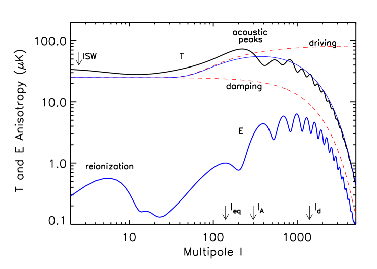
Figure 1: Temperture and E-type polarization anisotropies versus the multipole number, for a flat $\Lambda$CDM model, consistent with WMAP and computed using CMBFAST cmbfast . The parameters are: $\Omega_{b}=0.046,\Omega_{m}=0.27,\Omega_{\Lambda}=0.73,h=0.72,n_{s}=0.99$. Some of the effects discussed in the text are marked in the figure, as well as the location of different characteristic scales $l_{eq}$, $l_{A}$ and $l_{D}$. Radiation driving leads to the rise of the temperature anisotropy above $l_{eq}$, while Silk damping and the damping due the finite thickness of the LSS causes the amplitude to fall for $l>l_{D}$. The forms for these envelopes are taken from hu_white97 . The ISW effect is important at small $l$. The early ISW effect is important around $l_{eq}$ and is one reason for the first peak’s shift to $l_{1}<l_{A}$. The polarization rises as $(l/l_{D})$ in the tight coupling limit, due to the small quadrupole source, and is also damped for $l>l_{D}$. The effect of reionization is to cause the rise of the polarization signals at low $l$. The figure is inspired by a similar figure in Hu hurev .

We show in Figure 1 a plot of the temperature anisotropy $\Delta T=T\sqrt{l(l+1)C_{l}/2\pi}$ and polarization anisotropy versus $l$, for a standard $\Lambda$CDM cosmology, got by running the publicly available code CMBFAST cmbfast . One sees a number of features in such a plot, a flat plateau at low $l$ rising to several peaks and dips, as well as a cut-off at high $l$. Our aim will be to develop a physical understanding of the various features that the figure displays. We now turn to the formalism for computing the $C_{l}$‘s for any theory.

III The Boltzmann equation

The distribution function for photons, $f(x^{i},p_{\beta})\equiv f({\bf x},{\bf p},\eta)$, is defined by giving their number in an infinitesimal phase space volume, $dN=f(x^{\alpha},p_{\beta},\eta)d^{3}x^{\alpha}d^{3}p_{\beta}$. Note that we will use Greek letters for purely spatial co-ordinates and Latin ones for space-time co-ordinates. We can write $dN$ in a co-ordinate independent way,

$$dN=\int_{p_{0}}\frac{d^{4}p_{k}}{\sqrt{-g}}\ f(x^{i},p_{j})\ p^{l}d\Sigma_{l}\ 2\delta[p_{m}p^{m}]$$ (9)

where $g$ is the determinant of the metric, $d\Sigma_{i}=\sqrt{-g}\ \epsilon_{ijkl}\ [dx^{i}\wedge dx^{j}\wedge dx^{k}]/3!$ is an infinitesimal spacelike hypersurface, $p_{i}$ the photon 4-momentum and the delta function ensures that $p_{i}$ is a null vector. To get the simple expression for $dN$, one chooses a time slicing with $d\Sigma_{i}\equiv(\sqrt{-g}dx^{1}dx^{2}dx^{3},0,0,0)$ and carries out the integral over $p_{0}$ retaining only the positive energy part of the delta function. This shows explicitly that $f$ is a co-ordinate invariant scalar field. Further, in the absence of collisions, both $dN$ and the phase-space volume $d^{3}x^{\alpha}d^{3}p_{\beta}$ would be conserved along the photon trajectory and hence also the phase space density $f$. If $\lambda$ is an affine parameter along the null geodesic, we will then have $df/d\lambda=0$. On the other hand when collisions are present the distribution function will change. This situation is generally handled by introducing a collision term on the RHS of the CBE, that is writing $df/d\lambda=\tilde{c}(f)$. Further it is generally convenient to use the time co-ordinate itself, say $\eta$, as the independent parameter along the photon trajectory and write $df/d\lambda=(d\eta/d\lambda)(df/d\eta)=\tilde{c}(f)=(d\eta/d\lambda)c(f)$. One then has

$${df\over d\eta}={\partial f\over\partial\eta}+{dx^{\alpha}\over d\eta}{\partial f\over\partial x^{\alpha}}+{dp_{\alpha}\over d\eta}{\partial f\over\partial p_{\alpha}}=c(f)$$ (10)

We look at this equation in the spatially flat, perturbed FRW universe. Its metric in the conformal-Newton gauge is

$$ds^{2}=a^{2}(\eta)\left[(1+2\phi)d\eta^{2}-(1-2\phi)(dx^{2}+dy^{2}+dz^{2})\right]$$ (11)

Here $a(\eta)$ is the expansion factor and $\eta$ is the conformal time, related to the proper time by $a(\eta)d\eta=dt$. (We adopt $c=1$ units). We have assumed that a single potential $\phi$ describes the scalar perturbation, which holds if the source of the perturbations is a perfect fluid with no off-diagonal components to the energy-momentum tensor.

Since the photon 4-momentum $p^{i}$ is a null vector we have $g^{ik}p_{i}p_{k}=0$. We choose the photon 4-momentum to have components $p_{i}\equiv(\sqrt{g^{\alpha\alpha}/g^{00}}\ p,-pn^{\alpha})$ where, we have defined the magnitude of the spatial component of (co-variant) momentum, $p=\Sigma_{\alpha}p_{\alpha}p_{\alpha}$. Also $\bm{n}$ is a unit vector in the direction of the photon 3-momentum $p^{\alpha}$.

Then to linear order in the perturbed potential,

$$\frac{dx^{\alpha}}{d\eta}={dx^{\alpha}/d\lambda\over d\eta/d\lambda}={p^{\alpha}\over p^{0}}=n^{\alpha}(1+2\phi).$$ (12)

The geodesic equation for the photons to the linear order in the perturbations is

$${dp_{i}\over d\eta}=2p{\partial\phi\over\partial x^{i}}.$$ (13)

The Boltzmann equation then becomes

$${df\over d\eta}={\partial f\over\partial\eta}+(1+2\phi)n^{\alpha}{\partial f\over\partial x^{\alpha}}+2p{\partial\phi\over\partial x^{\alpha}}{\partial f\over\partial p_{\alpha}}=c(f)$$ (14)

An observer at rest in the perturbed FRW universe, has a 4-velocity $u^{i}\equiv(1/\sqrt{g_{00}},0)$. So the energy of the photon measured by such an observer is $E=p_{i}u^{i}=p(1+\phi)/a$. In the unperturbed FRW universe, the energy simply redshifts with expansion with $E=p/a$. The distribution function for the photons, in the absence of perturbations is then described by the Planck law,

$$f_{b}\left(\frac{p}{T}\right)=\frac{A}{exp(p/T)-1}.$$ (15)

Defining the perturbed phase space density $f_{1}(\bm{x},p,\bm{n},\eta)=f(\bm{x},p,\bm{n},\eta)-f_{b}(p)$, to linear order the Boltzmann equation becomes

$${\partial f_{1}\over\partial\eta}+\bm{n}\cdot\bm{\nabla}f_{1}-2p\ \bm{n}\cdot\bm{\nabla}\phi{\partial f_{b}\over\partial p}=c(f)$$ (16)

where we have replaced $f$ by $f_{b}$ in the term last on the LHS of Eq. (14) and used $(\partial f_{b}/\partial p_{\alpha})=(p_{\alpha}/p)(\partial f_{b}/\partial p)=-n^{\alpha}(\partial f_{b}/\partial p)$.

In the perturbed FRW universe we note that both the perturbed trajectory and the effect of collisions (under the Thomson scattering approximation) do not depend on the photon energy. This motivates us to define the perturbed phase space density in terms of a purely temperature perturbation $\delta T(\bm{x},\eta,\bm{n})$ in $f_{b}$. We take

$$f({\bf x},p,{\bf n},\eta)=f_{b}\left[\frac{p}{T+\delta T(\bm{x},\eta,\bm{n})}\right].$$ (17)

(Note that in such an approximation, we are also neglecting the effects of any spectral distortion). To the first order in $\delta T/T$ one can expand $f$ in Eq. (17) to get $f_{1}=-p(\partial f_{b}/\partial p)(\delta T/T)$. Again because both the perturbed trajectory and the effect of collisions do not depend on $p$, we will usually integrate over $p$’s. It is then useful to deal with not the full phase space density, but just its associated fractional brightness perturbation defined by

$$i=\frac{\int f_{1}p^{3}dp}{\int f_{b}p^{3}dp}=4\frac{\delta T}{T}(\bm{x},\eta,\bm{n}).$$ (18)

To appreciate better the meaning of $(\delta T/T)=i/4$ let us look at the energy momentum tensor of the photons. This is

$$T^{i}_{j}=\int{d^{4}p_{k}\over\sqrt{-g}}\ p^{i}p_{j}2\ \delta(p^{m}p_{m})f=\int{d^{3}p_{\alpha}\over\sqrt{-g}}{p^{i}p_{j}\over p^{0}}f$$ (19)

The energy density in the perturbed FRW universe, with metric given by Eq. (11) is

$$\rho=T^{0}_{0}={(1+4\phi)\over a^{4}}\int p^{3}dp\ d\Omega\ f=\rho_{R}(1+4\phi)\left[1+\int i{d\Omega\over 4\pi}\right]$$ (20)

where $\rho_{R}=(4\pi/a^{4})\int p^{3}dpf_{b}(p)$ is the radiation energy density in the absence of perturbations. Let us define $i_{0}=\int i(d\Omega/4\pi)$ and $(\delta T/T)_{0}=\int(\delta T/T)(d\Omega/4\pi)$, the zeroth moments of the perturbed brightness $i$ and temperature $(\delta T/T)$ respectively, over the directions of the photon momenta. The fractional perturbation to the radiation energy density is given by

$$\delta_{R}={\rho-\rho_{R}\over\rho_{R}}=4\phi+i_{0}=4\left[\left(\frac{\delta T}{T}\right)_{0}+\phi\right]$$ (21)

Note that in the conformal Newton gauge the radiation density perturbation has an additional contribution from the perturbed potential itself (over and above the contribution from the perturbed distribution function). One may feel that this differs from the naive expectation that the radiation energy density to vary as $\rho\propto T^{4}$ and hence the ’physical’ temperature perturbation go as just $(1/4)\delta\rho/\rho$. Since the energy of a photon seen by an observer at rest in the perturbed FRW universe is $E=p(1+\phi)/a$ (see above), one can write the phase space density in the perturbed FRW universe, to linear order as

$$f=f_{b}\left(\frac{p}{\,{\rm T}+\delta T}\right)=f_{b}\left(\frac{Ea}{(\,{\rm T}+\delta T)(1+\phi)}\right)=f_{b}\left(\frac{Ea}{\,{\rm T}+(\delta T+\phi)}\right).$$ (22)

This shows that $\Theta=\delta T+\phi$ is indeed the ’physical’ temperature perturbation measured by an observer at rest in the perturbed FRW universe and that $\Theta_{0}=\int\Theta(d\Omega/4\pi)=\delta_{R}/4$, as expected.

IV The collision term and the equation for the perturbed brightness

We now consider the effect of collisions. The process that we wish to take into account is the scattering between photons and electrons. In fact to linear order it is sufficient to consider the Thomson scattering limit of negligible energy transfer in the electron rest frame. Since the distribution function is a scalar, the effects of collision are most simply calculated by going to the electron (or fluid) rest frame and transferring the results to any other co-ordinate frame. Suppose the distribution function changes by $df=d\bar{f}=d\tau\bar{c}$ in the fluid rest frame. Henceforth quantities with an ’overbar’ will represent variables in the fluid rest frame. Then one can write $df/d\eta=(d\tau/d\eta)\bar{c}$. The differential cross section for Thomson scattering of unpolarized radiation is given by

$$\frac{d\sigma}{d\Omega^{\prime}}=\frac{\sigma_{T}}{4\pi}\left(1+\frac{P_{2}(\bar{\bm{n}}\cdot\bar{\bm{n}}^{\prime})}{2}\right)$$ (23)

where $\sigma_{T}$ is the Thomson cross section and $\bar{\bf n}$ and $\bar{\bf n}^{\prime}$ are the unit vectors specifying the direction of the initial and the scattered photon momenta in the fluid rest frame. The collision term $df/d\tau=d\bar{f}/d\tau=\bar{c}$ will have a source due to the photons scattered into the beam from a direction $\bar{\bm{n}}^{\prime}$ and a sink due to scattering out of the beam. So we have

$$\bar{c}(\bar{f})=n_{e}\sigma_{T}\int\frac{d\Omega^{\prime}}{4\pi}\left[1+\frac{P_{2}(\bar{\bm{n}}\cdot\bar{\bm{n}}^{\prime})}{2}\right]\left[\bar{f}(\bar{p},\bar{\bm{n}}^{\prime})-\bar{f}(\bar{p},\bar{\bf n})\right]$$ (24)

where the integration over $d\Omega^{\prime}$ is over the directions of $\bar{\bf n}^{\prime}$.

In order to derive the equation satisfied by the brightness perturbation we multiply the linearized Boltzmann equation (16) by $p^{3}$ and integrate over $p$ to get

$${\rho_{R}a^{4}\over 4\pi}\left[{\partial i\over\partial\eta}+{\bf n}.\nabla i+8{\bf n}.\nabla\phi\right]={d\tau\over d\eta}\int p^{3}dp\ \bar{c}(\bar{f})$$ (25)

We simplify the collision term on the RHS of Eq. (25), in Appendix A. From Eq. (25), Eq. (80) and Eq. (81) the equation satisfied by $i$, to the leading order of the perturbations, is given by

$${\partial i\over\partial\eta}+{\bf n}.\nabla i+8{\bf n}.\nabla\phi=n_{e}\sigma_{T}a\left[i_{0}+4{\bf n}.{\bf v}+\frac{1}{10}\sum_{m}Y_{2m}(\bm{n})i_{2m}-i\right].$$ (26)

The effects of Thomson scattering is to drive the photon distribution such that the RHS of Eq. (26) would vanish. If the scattering cross section had been isotropic, then $i$ would have been driven to $i_{0}$ in the fluid rest frame; but in the frame where the fluid moves there is a doppler shift. In addition the anisotropy of Thomson scattering introduces the dependence on the quadrupole moment of the brightness. The perturbed brightness equation will be used to derive the equation for the CMBR anisotropies, and also the dynamics for the baryon photon fluid.

V Integral solution for CMBR anisotropies

Consider the perturbed brightness equation Eq. (26) in Fourier space, in terms of the Fourier coefficients $\hat{\Theta}(\bm{k},\eta,\bm{n})$ of the ’physical’ temperature perturbation $\Theta=\delta T/T+\phi=i/4+\phi$, that is

$$\Theta(\bm{x},\eta,\bm{n})=\int\frac{d^{3}\bm{k}}{(2\pi)^{3}}e^{\mathrm{i}\bm{k}\cdot\bm{x}}\hat{\Theta}(\bm{k},\eta,\bm{n}).$$ (27)

Henceforth we shall denote the Fourier transform of any quantity $A$ by $\hat{A}$, except for the velocity ($\bm{v}$) and potential ($\phi$) whose Fourier transforms are denoted by $\bm{V}$ and $\Phi$ respectively. We also assume that these Fourier co-efficients depend on $\bm{n}$ only through $\mu=\hat{\bm{k}}\cdot\bm{n}$, as will obtain for example for scalar perturbations. In this case one can choose an axis for each $\bm{k}$ mode such that $i_{2m}=0$ for $m\neq 0$ and $\sum_{m}Y_{2m}(\bm{n})\hat{i}_{2m}/10=-\hat{\Theta}_{2}P_{2}(\mu)/2$, where

$$\Theta(\bm{k},\eta,\mu)=\sum_{l}(-\mathrm{i})^{l}(2l+1)\hat{\Theta}_{l}(\bm{k},\eta)P_{l}(\mu)$$ (28)

is the expansion of $\hat{\Theta}$ in a Legendre series. For scalar perturbations, $\bm{V}$ is also parallel to the $\bm{k}$ vector, and so $\bm{n}\cdot\bm{V}=(\bm{n}\cdot\hat{\bm{k}})V=V\mu$. Further, it is much more convenient to work with the equation for the combination $\hat{\Theta}+\Phi$. From the Fourier transform of Eq. (26) we then have

$$(\dot{\hat{\Theta}}+\dot{\Phi})+(\mathrm{i}k\mu+n_{e}\sigma_{T}a)[\hat{\Theta}+\Phi]=n_{e}\sigma_{T}a\ S(\bm{k},\eta,\mu)+2\dot{\Phi},$$ (29)

where, henceforth an over dot will denote a partial derivative, i.e. $\dot{f}=\partial f/\partial\eta$, for any $f$. We have also defined the source function

$$S(\bm{k},\eta,\mu)=\left[\hat{\Theta}_{0}+\Phi+V\mu-\frac{P_{2}(\mu)\hat{\Theta}_{2}}{2}\right]$$ (30)

Suppose we define the differential optical depth to electron scattering $d\tau=n_{e}\sigma_{T}a\ d\eta=n_{e}\sigma_{T}dt$. Then one can solve Eq. (29) formally as

$$\hat{\Theta}(\bm{k},\eta_{0},\mu)+\Phi(\bm{k},\eta_{0}) = [\hat{\Theta}(\eta_{i})+\Phi(\eta_{i})]e^{-ik\mu(\eta_{0}-\eta_{i})}e^{-\tau(\eta_{0},\eta_{i})}$$ (31)

$$+ \int_{\eta_{i}}^{\eta_{0}}d\eta\ e^{-\tau(\eta_{0},\eta)}\left[\dot{\tau}S({\bf k},\eta^{\prime},{\bf n})+2\dot{\Phi}\right]e^{-ik\mu(\eta_{0}-\eta)}$$

where we have defined the optical depth to electron scattering between epochs $\eta$ to the present $\eta_{0}$

$$\tau(\eta_{0},\eta)=\int_{\eta}^{\eta_{0}}d\eta^{\prime}n_{e}(\eta^{\prime})\sigma_{T}a(\eta^{\prime}),$$ (32)

and $\dot{\tau}(\eta)=d\tau(\eta,\eta^{\prime})/d\eta=n_{e}(\eta)\sigma_{T}a(\eta)$. The first term on the RHS of Eq. (31) can be neglected by taking a small enough initial time $\eta_{i}$, because the exponential damping for large optical depths. One can then simplify Eq. (31) to get at the present epoch $\eta_{0}$

$$\hat{\Theta}(\bm{k},\eta_{0},\mu)+\Phi(\bm{k},\eta_{0})=\int_{\eta_{i}}^{\eta_{0}}d\eta\ S(\bm{k},\eta,\mu)g(\eta_{0},\eta)e^{-ik\mu(\eta_{0}-\eta)}+2\int_{\eta_{i}}^{\eta_{0}}d\eta\ \dot{\Phi}\ e^{-ik\mu(\eta_{0}-\eta)}e^{-\tau(\eta_{0},\eta)}.$$ (33)

We have defined above the visibility function

$$g(\eta_{0},\eta)=\dot{\tau}(\eta)e^{-\tau(\eta_{0},\eta)}=n_{e}(\eta)\sigma_{T}a(\eta)\ \exp\left[-\int_{\eta}^{\eta_{0}}d\eta^{\prime}n_{e}(\eta^{\prime})\sigma_{T}a(\eta^{\prime})\right],$$ (34)

such that $g(\eta_{0},\eta)d\eta$ gives for every $\eta_{0}$ the probability that the last scattering of a photon occurred in the interval $(\eta,\eta+d\eta)$. Suppose $\eta_{0}$ is the conformal time at the present epoch. Then as $\eta$ decreases from $\eta_{0}$, the optical depth to electron scattering will increase and so will $g$. However far back into the past when $\tau\gg 1$, $g$ will be exponentially damped. So the visibility function generally increases as one goes into the past attains a maximum at an ’epoch of last scattering’ and decreases exponentially thereafter. Its exact behavior of course depends on the evolution of the free electron number density during the recombination epoch and also on the subsequent ionization history of the universe. If the universe went through a standard recombination epoch with no significant reionization thereafter, then the ’surface of last scattering’ is centered at $z\approx 1100$ with a very small half width $\Delta z\approx 100$. If on the other hand the universe got significantly reionized at high redshifts, as it seems to be indicated by the WMAP observations, some fraction $\tau_{ri}\sim 0.17$, of the photons will suffer last scattering surface at later epochs.

We can calculate $a_{l}(\bm{k},\eta_{0})$ by taking the Legendre transform of both sides of Eq. (33). Note that the term $\Phi({\bf k},\eta_{0})$ on the LHS of Eq. (33), does not depend on the photon direction and so does not contribute to CMBR anisotropy at all. Using the expansion of plane-waves in terms of spherical waves,

$$e^{-ik\mu x}=\sum_{l}(-\mathrm{i})^{l}(2l+1)j_{l}(x)P_{l}(\mu),$$ (35)

and writing $\mu\exp(-\mathrm{i}\mu kx)=id(\exp(-\mathrm{i}\mu kx))/d(kx)$, we get

$$a_{l}(\bm{k},\eta_{0})=\int_{0}^{\eta_{0}}d\eta g(\eta_{0},\eta)\left[(\hat{\Theta}_{0}+\Phi)j_{l}(k\Delta\eta)+\mathrm{i}Vj_{l}^{\prime}(k\Delta\eta)+\frac{\hat{\Theta}_{2}}{2}\ \frac{\left(3j_{l}^{\prime\prime}(k\Delta\eta)+j_{l}(k\Delta\eta)\right)}{2}\right]$$ (36)

$$+\int_{0}^{\eta_{0}}d\eta\ e^{-\tau(\eta_{0},\eta)}2\dot{\Phi}j_{l}(k\Delta\eta)$$

Here $j_{l}(kx)$ is the spherical Bessel function, and $j_{l}^{\prime}$ denotes a derivative with respect to the argument, $\Delta\eta=\eta_{0}-\eta$.

Let us interpret the various terms in Eq. (36). This equation shows that anisotropies in the CMBR result from a combination of radiation energy density perturbations $\hat{\Theta}_{0}$ and potential perturbations $\Phi$ (the monopole term), on the last scattering surface and the doppler effect due to the line of sight component of the baryon velocity $V$ (the dipole term). The anisotropy of the Thomson scattering cross section also leads to a dependence on the radiation quadrupole $\hat{\Theta}_{2}$. The spherical Bessel function and its derivatives in front of these terms project variations in space, at the conformal time $\eta$ around last scattering, to the angular (or $l$) anisotropies at the present epoch $\eta_{0}$. (A popular jargon is to say that the monopole, dipole and quadrupole at last scattering free stream to produce the higher order multipoles today). These spherical Bessel functions generally peak around $k\Delta\eta\approx l$. The multipoles $l$ are then probing generally spatial scales with wavenumber $k\sim l/\Delta\eta$ at around last scattering. The visibility function weighs the contribution at any conformal time $\eta$ by the probability of last scattering from that epoch. Finally, the last term ($\dot{\Phi}$ term) shows that any variation of the potential along the line of sight will also lead to CMBR anisotropies, and is usually referred to as the integrated Sachs-Wolfe (ISW) effect.

In the limit of a very narrow LSS at $\eta=\eta^{*}$, For angular scales (and $l$’s) such that, their associated spatial scales at the LSS are much larger than the LSS thickness, one can take the variation of the $j_{l}^{\prime}s$ with $\eta$ to be much slower than that of the visibility function. In such a narrow LSS approximation, we get

$$a_{l}(\bm{k},\eta_{0})=(\hat{\Theta}_{0}+\Phi)(\eta^{*})j_{l}(kR^{*})+\mathrm{i}V(\eta^{*})j_{l}^{\prime}(kR^{*})+\frac{\hat{\Theta}_{2}(\eta^{*})}{2}\ \frac{\left(3j_{l}^{\prime\prime}(kR^{*})+j_{l}(kR^{*})\right)}{2}+\int_{\eta^{*}}^{\eta_{0}}d\eta 2\dot{\Phi}j_{l}(k\Delta\eta),$$ (37)

where $R^{*}=\eta_{0}-\eta^{*}$ is the co-moving angular diameter distance to the LSS. Note that due to the presence of $e^{-\tau}$ in the in the last term, the range of integration is restricted to be from about $\eta^{*}$ to the present. The presence of a finite width of the LSS causes a contribution to the ISW effect from epochs just around last scattering as well, usually referred to as the early ISW effect. Once we calculate the photon brightness, and the baryon velocities at the epochs corresponding to last scattering, one can calculate $a_{l}$ using Eq. (36) and $C_{l}$ from Eq. (8). Before considering the dynamics of the the baryon-photon fluid in detail, let us first use the Eq. (37) to calculate the CMBR anisotropies at large angular scales.

VI Sachs-Wolfe effect and large angle anisotropies

We wish to calculate the anisotropies generated at large angular scales (or small values of $l$), large enough such that the associated spatial scales are larger than the Hubble radius at the LSS (i.e. $k\eta^{*}\ll 1$). For such scales one can neglect the thickness of the LSS and calculate $a_{l}$ using Eq. (37). Let us also assume that the universe is spatially flat and that it is matter dominated by the time $\eta=\eta^{*}$. The evolution of the gravitational potential $\phi$ is considered in detail in the review by Mukhanov et al. MBF for a variety of initial conditions, and in various epochs. We will draw upon several of their results below.

VI.1 Adiabatic perturbations

Consider first adiabatic (or isentropic) perturbations, for which $\delta\rho_{n}/(\rho_{n}+p_{n})$ is the same initially for all components. (Here $p_{n}$ is the pressure of component $n$). This condition is preserved by the evolution on super Hubble scales MBF . As we show below, it is also preserved in the evolution of the tightly-coupled baryon-photon fluid. For a flat matter dominated universe, the potential evolves as $\ddot{\phi}+(6/\eta)\phi=0$, which implies that $\phi$ is constant in time, ignoring the decaying mode MBF . A detailed calculation starting from an initial potential perturbation $\phi_{i}$ and following the evolution of the adiabatic mode from radiation era through the matter radiation equality gives, $\phi=(9/10)\phi_{i}\equiv\phi_{0}$. The perturbed Einstein equation also gives for the matter density perturbation MBF , $\delta_{m}=-2\phi+(\eta^{2}/6)\nabla^{2}\phi$, and $\bm{v}=-(1/3)\eta\bm{\nabla}\phi$. For adiabatic perturbations $\delta_{R}=(4/3)\delta_{m}$. So $\Theta_{0}=\delta_{R}/4=\delta_{m}/3=-(2/3)\phi+(\eta^{2}/18)\nabla^{2}\phi\to-(2/3)\phi$, for large scales, such that $k\eta\ll 1$. So the Fourier co-efficient $\hat{\Theta}_{0}+\Phi=-(2/3)\Phi+\Phi=\Phi/3$. Further since $V=-(\mathrm{i}/3)(k\eta)\Phi$, this dipole term in Eq. (37) is negligible compared to the monopole term $\hat{\Theta}_{0}+\Phi$. Also because of tight coupling and negligible thickness to the LSS there is negligible quadrupole component to $\hat{\Theta}_{2}$ for $k\eta\ll 1$. On super Hubble scales, for adiabatic perturbations one then has

$$a_{l}=a_{l}^{SW}=\frac{1}{3}\Phi_{0}\ j_{l}(kR^{*});\quad C_{l}^{SW}=\frac{2}{\pi}\int{dk\over k}\frac{k^{3}\langle|\Phi_{0}(k)|^{2}\rangle}{9}\ j_{l}^{2}(kR^{*})$$ (38)

The above $C_{l}$, which describes the CMBR anisotropies on large scales due to initially adiabatic potential perturbations, was first derived by Sachs and Wolfe SW67 and is referred to as the Sachs-Wolfe effect. For a power law spectrum of potential perturbations, with $\Delta_{\phi}^{2}=k^{3}|\Phi_{0}(k)|^{2}/(2\pi^{2})=A_{\phi}^{2}(k_{0})(k/k_{0})^{n_{s}-1}$, one gets

$$C_{l}^{SW}=\frac{2A_{\phi}^{2}}{9}\left(\frac{1}{k_{0}R^{*}}\right)^{n_{s}-1}\frac{2^{n_{s}-4}\Gamma(3-n_{s})\Gamma((2l+n_{s}-1)/2)}{\Gamma^{2}((4-n_{s})/2)\Gamma((2l+5-n_{s})/2)}.$$ (39)

(In the above equation $\Gamma(x)$ is the usual gamma function). In theories of inflation, one obtains a nearly scale invariant spectrum corresponding to $n_{s}=1$. For this case, one gets a constant

$$\frac{l(l+1)C_{l}^{SW}}{2\pi}=\left(\frac{A_{\phi}}{3}\right)^{2}.$$ (40)

It is this constancy of $(l(l+1)C_{l})/2\pi$ for scale invariant spectra that motivates workers in the field to use this combination to present their results. For power law spectra, the recent WMAP results by themselves, favor a nearly scale invariant spectral index with $n_{s}=0.99\pm 0.04$, but when other large scale structure data is added slightly lower values of $n_{s}$ are favored spergel03 . Spergel et al spergel03 also explore more complicated, running spectral index models, for fitting the results from WMAP, other fine scale CMB experiments and large scale structure data. A recent study combining CMB and large scale structure data favors a scale invariant spectrum, with $n_{s}=0.98\pm 0.02$ with $dn_{s}/d\ln k=0.003\pm 0.01$i seljaketal . Slightly different set of parameters are derived by tegmark04 , when they combine the WMAP data with the SDSS results.

One can relate the normalization constant $A_{\phi}$ to the scalar normalization $A$ used in CMBFAST and by the above authors. Verde et al verde03 give $\Delta_{\phi}^{2}(k_{0})=(800\pi^{2}/T)A^{2}$, where $T=2.725\times 10^{6}\mu\,{\rm K}$ and $k_{0}=0.002\,{\rm Mpc}^{-1}$. For $n=1$, and adopting a value $A=0.9$, the best fit value for WMAP data alone, gives $A_{\phi}\sim 3\times 10^{-5}$, in agreement with the earlier COBE results. We can also relate $A_{\phi}$ to the normalization of the matter power spectrum $\delta_{H}^{2}=k^{3}P(k)/(2\pi^{2})$, evaluated at $k=H_{0}$. We have $\delta_{H}=(2/3)A_{\phi}(D_{1}(a=1)/\Omega_{m})^{1/2}$, where $D_{1}(a)$ is the growth factor dodelson . For a flat matter dominated model one would then get $\delta_{H}\sim 2\times 10^{-5}$ consistent with earlier COBE results.

VI.2 The isocurvature mode

The Sachs-Wolfe effect in theories which begin initially with isocurvature perturbations can be computed in an analogous manner. Suppose for example, one assumes that the universe has two dominant components, radiation with density $\rho_{R}$ and dark matter with density $\rho_{m}$. Then the total density perturbation will be $\delta_{T}=(\rho_{R}\delta_{R}+\rho_{m}\delta_{m})/(\rho_{R}+\rho_{m})=(\delta_{R}+y\delta_{m})/(1+y)$. Here we have defined $y=\rho_{m}/\rho_{R}=a(\eta)/a(\eta_{eq})$ with $\eta_{eq}$ the epoch of matter-radiation equality. In such a model there is also an independent ’isocurvature’ mode, where the initial curvature fluctuation is zero, but there are non-zero fluctuations in the ’entropy per particle’, $S\propto n_{R}/n_{m}\propto T^{3}/\rho_{m}$. This entropy fluctuation is characterized by $\sigma=\delta S/S=3\Theta_{0}-\delta_{m}$. In terms of $\delta_{T}$ and $\sigma$, we have $\delta_{R}=(\delta_{T}(1+y)+y\sigma)/(1+3y/4)$. For such isocurvature initial conditions on super Hubble scales, the initial value of $\sigma=\sigma_{i}$ is preserved, and this drives the generation of curvature or potential perturbations in the radiation dominated era (see for example MBF ). The resulting potential fluctuations freeze after matter domination, on super Hubble scales, and are given by $\phi=\sigma_{i}/5$ with an associated density perturbation $\delta_{T}=-2\phi=-2\sigma_{i}/5$. Also at matter domination, with $y\gg 1$, one has $\delta_{R}\to(4/3)(\delta_{T}+\sigma)$. So $\Theta_{0}=\delta_{R}/4\to(1/3)(-2\phi+5\phi)=\phi$ and $\Theta_{0}+\phi=2\phi$. Then the associated CMBR anisotropies due to the monopole term in Eq. (37) is $a_{l}=(\hat{\Theta}_{0}+\Phi)j_{l}(kR^{*})=2\Phi j_{l}(kR^{*})$. The associated dipole and quadrupole can again be neglected for super horizon scales. For the same amplitude of potential perturbations at the epoch of last scattering, isocurvature initial conditions therefore lead to $6$ times larger temperature anisotropies on large scales. We have considered here only a two component system; for several components, several independent modes of perturbations can obtain with a variety of associated CMBR anisotropies mood_buc_tur .

VI.3 The integrated Sachs-Wolfe effect

If the potential $\phi$ were to change with time after decoupling, we see from Eq. (37) that further anisotropies can be generated at large angular scales. This effect is known as the integrated Sachs Wolfe effect, and typically arises in open universes, or in a flat universe with dark energy/cosmological constant, wherein the potential decays after the universe is dominated by curvature or dark energy respectively. The gravitational potential is also traced by other measures of large scale structure, There has therefore been considerable interest in checking whether there is a large angle cross-correlation between the temperature anisotropies (some of which will arise due the ISW effect) and other measures of large scale structure, with some tentative detections isw_de .

The Sachs-Wolfe and the ISW effects are dominant on scales larger than a few degrees, or $l<20$ or so as schematically indicated in Figure 1. In order to understand the smaller scale anisotropies we have to have study in greater detail the baryon-photon dynamics, to which we now turn.

VII The Baryon-Photon dynamics

We have already derived the equation for the perturbed brightness for the photons. To complete the description of the baryon-photon system we have to also write down the continuity and Euler equations for the Baryons in the perturbed FRW universe. The continuity equation for the baryon density perturbation $\delta_{B}$ is

$$\dot{\delta}_{B}+\bm{\nabla}\cdot\bm{v}=3\dot{\phi}$$ (41)

where term on the RHS takes account of the variation of the spatial volume due to the perturbed potential. In the baryon Euler equation, we include the force exerted by the radiation on the Baryons due to $\gamma-e$ collisions. This force is most simply calculated as the negative of the rate of momentum density transfer to the photons by the electrons. The change in the momentum density of photons per unit conformal time to linear order in the perturbations is given by

$$\frac{dT_{0}^{\beta}}{d\eta}=\int\frac{d^{3}p_{\alpha}}{\sqrt{-}g}\frac{p^{\beta}p_{0}}{p^{0}}\left(\frac{df}{d\eta}\right)_{coll}=\frac{1}{a^{4}}\int p^{3}dpd\Omega n^{\beta}\ c(f)$$ (42)

where $(df/d\eta)_{coll}=c(f)$ is the change in photon momentum density due to collisions calculated in Section IV. The momentum transfer to the electrons will be negative of the value calculated in Eq. (42). The radiative force density exerted on the electrons (and hence the baryons) by the radiation is then

$$\bm{f}_{rad}=-\frac{4\pi}{a^{4}}\int\frac{d\Omega}{4\pi}\left[n_{e}\sigma_{T}a\frac{\rho_{R}a^{4}}{4\pi}\left(i_{0}+\frac{i_{2m}Y_{2m}}{10}+4\bm{n}\cdot\bm{v}-i\right)\bm{n}\right]=n_{e}\sigma_{T}\rho_{R}a\left[\bm{F}-\frac{4}{3}\bm{v}\right]$$ (43)

where $\bm{F}=\int(d\Omega/4\pi)\ i\ \bm{n}$ is the first moment over photon directions of the fractional brightness. So the baryons feel a force due to the radiative flux $\bm{F}$ and a drag proportional to their velocity. The Euler equation for the baryons is then

$$\rho_{B}[\dot{\bm{v}}+{\cal H}\bm{v}]=-\rho_{B}\nabla\phi-\nabla p_{B}+n_{e}\sigma_{T}\rho_{R}a\left[{\bf F}-{4\over 3}{\bf v}\right]$$ (44)

where ${\cal H}=(da/d\eta)/a$ and $p_{B}$ is the baryon pressure. The equations Eq. (26), Eq. (41). Eq. (44) together with an equation of state for the Baryon gas form the basic set of equations for the Baryon-Photon system. These equations can be solved to a good approximation in the tight coupling limit, where we consider scales of the perturbations much larger than the photon mean-free path. This approximation is likely to be very accurate, before the recombination epoch, when matter is mostly in an ionized form. Note that the co-moving photon mean free path $L_{\gamma}=(n_{e}\sigma_{T}a)^{-1}$ grows to about $\,{\rm Mpc}$ scales just before the decoupling epoch. So the approximation $kL_{\gamma}\ll 1$ (which corresponds to the limit $l=kR^{*}\ll R^{*}/L_{\gamma}\sim 10^{4}$), should hold quite accurately for most scales of interests probed by CMBR anisotropies. One can then solve for the brightness perturbation iteratively. For this we first rewrite equation Eq. (26) as

$$i=i_{0}+{i_{2m}Y_{2m}\over 10}+4\bm{n}\cdot\bm{v}-L_{\gamma}\left[\frac{\partial i}{\partial\eta}+\bm{n}\cdot\bm{\nabla}i+8\bm{n}\cdot\bm{\nabla}\phi\right].$$ (45)

(The repeated $m$ index is assumed to be summed over). We can now write down the solution by iteration in powers of $L_{\gamma}$. We get

$$i^{(0)}=i_{0}+{i_{2m}Y_{2m}\over 10}+4\bm{n}\cdot\bm{v}$$ (46)

$$i^{(1)}=i^{(0)}-L_{\gamma}\left[\frac{\partial i^{(0)}}{\partial\eta}+\bm{n}\cdot\bm{\nabla}i^{(0)}+8\bm{n}\cdot\bm{\nabla}\phi\right]$$ (47)

Here $i^{(0)}$ and $i^{(1)}$ are iterative solutions to Eq. (45) giving $i$ to the zeroth and first order in $L_{\gamma}$, respectively. (We will later consider iteration up to the second order when deriving Silk damping).

Consider to begin with the effects of the baryon - photon tight coupling to the first nontrivial order given by $i^{(1)}$. Taking the zeroth moment of Eq. (47), that is averaging both sides of Eq. (47) over the all directions of the photon momentum, we get

$$i_{0}=i_{0}-L_{\gamma}\left[\frac{\partial i_{0}}{\partial\eta}+\frac{4}{3}\bm{\nabla}\cdot\bm{v}\right],$$ (48)

where we have used the fact that $\int(d\Omega/4\pi)n_{i}n_{j}=(1/3)\delta_{ij}$. Using $\Theta_{0}=i_{0}/4+\phi$, we then have

$$\frac{\partial\Theta_{0}}{\partial\eta}+\frac{1}{3}\bm{\nabla}\cdot\bm{v}=\dot{\phi}$$ (49)

This implies that the fractional perturbation to the photon number density $\delta n_{R}/n_{R}=3\Theta_{0}$ satisfies the same equation as $\delta_{B}$. So initially adiabatic perturbations in the baryons, with $\delta_{B}=3\Theta_{0}=(3/4)\delta_{R}$ initially, maintain this relation in the radiation era.

The first moment, (that is multiplying Eq. (47) by ${\bf n}$ and integrating over the directions of photon momenta) gives

$$\bm{F}=\frac{4}{3}\bm{v}-L_{\gamma}\left[{\nabla i_{0}\over 3}+{4\over 3}\dot{\bm{v}}+{8\over 3}\nabla\phi\right]$$ (50)

The radiative force experienced by the baryons is then

$$\bm{f}_{rad}=\frac{\rho_{R}}{L_{\gamma}}\left[\bm{F}-{4\over 3}\bm{v}\right]=-\rho_{R}\left[{\nabla i_{0}\over 3}+{4\over 3}\dot{\bm{v}}+{8\over 3}\nabla\phi\right]$$ (51)

So the Euler equation for the baryons, after substituting $\Theta_{0}=i_{0}/4+\phi$, becomes

$$[\rho_{B}+{4\over 3}\rho_{R}]\dot{\bm{v}}+\rho_{B}{\cal H}\bm{v}=-[\rho_{B}+{4\over 3}\rho_{R}]\bm{\nabla}\phi-\bm{\nabla}(p_{B}+\rho_{R}{4\Theta_{0}\over 3})$$ (52)

We see therefore that in the tight coupling limit, the effect of Thomson scattering by radiation, to the leading order, is to add to the baryon Euler equation : (i) a radiation pressure gradient term with $p_{rad}=\rho_{R}4\Theta_{0}/3=\rho_{R}\delta_{\gamma}/3$, (ii) an extra inertia due to the radiation by adding a mass density $(4\rho_{R}/3)$, to the inertial term in the LHS of Eq. (52) and to the gravitational force term on the RHS. When the radiation energy density and pressure dominate over that of matter, the baryon photon fluid, in the tight coupling limit, behaves as though its mass density is $(\rho_{R}+p_{R})$ and its pressure $p_{R}=\rho_{R}/3$ is due to radiation. The ratio of the inertia due to baryons and that due to radiation is given by $R=3\rho_{B}/4\rho_{R}\approx 0.6(\Omega_{b}h^{2}/0.02)(z/10^{3})^{-1}$. So baryon inertia cannot be neglected. (On the other hand the fluid pressure can be neglected compared to the radiation pressure, since the thermal speed in the fluid is much smaller than $c/\sqrt{3}$).

On taking the time derivative of the continuity equation Eq. (49), substituting for $\dot{\bm{v}}$ from the Euler equation Eq. (52), and taking its Fourier transform, we get

$$\frac{\partial^{2}\hat{\Theta}_{0}}{\partial\eta^{2}}+\frac{\dot{R}}{1+R}\frac{\partial\hat{\Theta}_{0}}{\partial\eta}+\frac{k^{2}\hat{\Theta}_{0}}{3(1+R)}=-\frac{k^{2}\Phi}{3}+\ddot{\Phi}+\frac{\dot{R}}{1+R}\dot{\Phi}$$ (53)

We see that the baryon photon fluid can undergo acoustic oscillations, driven by the potential, and with an effective sound speed $c_{s}=1/\sqrt{3(1+R)}$. If the baryon inertia were subdominant, with $R\to 0$, $c_{s}\to 1/\sqrt{3}$ which is the sound speed for a highly relativistic fluid. The baryon inertia leads to a reduction of $c_{s}$ from this extreme relativistic value. The oscillator equation Eq. (53) can also be cast in a more suggestive form (cf.Eq. 16 of hudodr ),

$$c_{s}^{2}\frac{\partial}{\partial\eta}\left(c_{s}^{-2}\frac{\partial\hat{\Theta}_{0}}{\partial\eta}\right)+c_{s}^{2}k^{2}\hat{\Theta}_{0}=-\frac{k^{2}\Phi}{3}+c_{s}^{2}\frac{d}{d\eta}\left(c_{s}^{-2}\dot{\Phi}\right).$$ (54)

We will use the solution of the oscillator equation Eq. (53) to discuss the imprint of the acoustic waves on $C_{l}$.

VIII Acoustic peaks

The acoustic oscillations of the baryon-photon fluid lead to a rich structure of peaks and troughs in the CMB anisotropy power spectrum, on sub degree angular scales (or $l>100$). To understand their basic features, let us look at an approximate solution of the oscillator equation Eq. (53). To begin with let us neglect the slow variation of $R$ with time, compared to the oscillation frequency $kc_{s}$. Then we can rewrite Eq. (53) as

$$\frac{\partial^{2}(\hat{\Theta}_{0}+\Phi)}{\partial\eta^{2}}+k^{2}c_{s}^{2}(\hat{\Theta}_{0}+\Phi)=-k^{2}c_{s}^{2}R\Phi+2\frac{\partial^{2}\Phi}{\partial\eta^{2}}$$ (55)

Also consider first modes which enter the Hubble radius in the matter dominated era, for which $(\partial^{2}\Phi)/\partial\eta^{2}\approx 0$. Then the solution of Eq. (55) is

$$\hat{\Theta}_{0}+\Phi=A(k)\cos kr_{s}(\eta)+B(k)\sin kr_{s}(\eta)-R\Phi$$ (56)

where $r_{s}(\eta)=\int_{0}^{\eta}d\eta^{\prime}/\sqrt{3(1+R)}$ is called the ’sound horizon’. Note the sine and cosine oscillations will persist in the full solution but will have a slow damping due to a variable $R$. The $-R\Phi$ term is the particular solution of the inhomogeneous equation. The effect of a non-zero $R$ (called ’baryon loading’) is to change the sound speed $c_{s}$ and also shift the zero point of the oscillations of the monopole $(\hat{\Theta}_{0}+\Phi)$. One needs to specify initial conditions to fix $A(k)$ and $B(k)$ in Eq. (56). Note that as $\eta\to 0$, for adiabatic or curvature perturbations, we already showed in Section VI that $\hat{\Theta}_{0}+\Phi\to\Phi/3$. This fixes $A(k)=(\Phi/3)(1+3R)$. Also in the tight coupling limit, we have from Eq. (49), $\mathrm{i}kV=-\partial\hat{\Theta}/\partial\eta$. Using this relation, and noting from Section VI that for adiabatic initial conditions $V\to 0$ as $k\eta\to 0$, fixes $B(k)=0$. Imposing these initial conditions we have for modes which enter in the matter dominated era,

$$\hat{\Theta}_{0}+\Phi=\frac{\Phi}{3}(1+3R)\cos kr_{s}-R\Phi;\qquad\mathrm{i}V=-\frac{3}{k}\frac{\partial\hat{\Theta}}{\partial\eta}=\Phi\frac{1+3R}{\sqrt{3(1+R)}}\sin kr_{s}$$ (57)

where we have again neglected the time variation of $\Phi$ and $R$.

VIII.1 Radiation driving

For modes which enter the Hubble radius during the radiation dominated era, one cannot neglect the variation in the gravitational potential $\Phi$. The comoving wavenumber $k_{eq}$, corresponding to the Hubble radius at matter-radiation equality, is $k_{eq}=H(z_{eq})/(1+z_{eq})=(2\Omega_{m}H_{0}^{2}z_{eq})^{1/2}$, and modes with $k>k_{eq}$ enter the Hubble radius in the radiation dominated era. During radiation domination, for the fluid which has an equation of state $p=\rho/3$, as would obtain for the tightly coupled baryon-photon fluid, the Einstein equations give $\ddot{\Phi}+(4/\eta)\dot{\Phi}+(k^{2}/3)\Phi=0$ (dots as before denote derivatives with respect to conformal time) MBF . The solution for ’adiabatic’ initial condition is

$$\Phi(k,\eta)=\frac{3}{(\omega\eta)^{3}}\left[\sin\omega\eta-\omega\eta\cos\omega\eta\right]\Phi_{i}(k)$$ (58)

where $\omega=k/\sqrt{3}=kc_{s}$ is the frequency of the acoustic waves and $\Phi_{i}(k)$ the initial potential perturbation on super horizon scales. (Note that during radiation domination $c_{s}=1/\sqrt{3}$). One sees that at early times on super horizon scales, with $k\eta\ll 1$, $\Phi\to\Phi_{i}$ where as once a mode enters the Hubble radius, the potential decays with time, going asymptotically as $\Phi(k,\eta)\to-(3\cos\omega\eta)\Phi_{i}/(\omega\eta)^{2}$ for $k\eta\gg 1$. This decay of $\Phi$ causes extra driving of the acoustic oscillations for such modes. We can estimate the effect of this extra driving by directly solving for the associated density perturbation $\delta_{R}=\delta\rho_{R}/\rho_{R}$ using the Einstein equations (cf. MBF ); $4\pi Ga^{2}\delta\rho_{R}=-k^{2}\Phi-3{\cal H}\dot{\Phi}-3{\cal H}^{2}\Phi$, and $3{\cal H}^{2}=8\pi Ga^{2}\rho_{R}$. For $k\eta\ll 1$ one gets $\delta_{R}\to-2\Phi_{i}$, giving an initial value for the monopole $(\hat{\Theta}_{0}+\Phi)=\delta_{R}/4+\Phi\to\Phi_{i}/2$. On the other hand, after a mode enters the Hubble radius, one has asymptotically, $\delta_{R}\to-(2k^{2}\eta^{2}/3)\Phi(k,\eta)=6\Phi_{i}(k)\cos(kc_{s}\eta)$ for $k\eta\gg 1$. So a mode which enters the Hubble radius early in the radiation dominated era has acoustic oscillations with

$$\hat{\Theta}_{0}+\Phi\to\hat{\Theta}_{0}=\delta_{R}/4=\frac{3}{2}\Phi_{i}(k)\cos kc_{s}\eta.$$ (59)

The amplitude of the oscillation, is therefore enhanced relative to a mode entering in the matter dominated era, by a factor $(3\Phi_{i}/2)/(\Phi_{0}/3)=5$, where we have used $\Phi_{0}=(9/10)\Phi_{i}$. This enhancement is referred to in the literature as ’radiation driving’ husug95 ; husugsil . The factor of $5$ derived above gets modified to about $4$, if we include the neutrino component husug95 . It is also valid only in the asymptotic limit of very small scales and ignores the damping effect to be discussed below. Further the modes which are seen as the first few peaks in the $C_{l}$ spectrum have $k/k_{eq}$ larger than unity only by a modest factor, and so the enhancement is smaller. Nevertheless, the rise from the Sachs-Wolfe plateau of the $C_{l}$ versus $l$ curve as $l$ increases from a few $10$’s to above $100$ or so, as displayed in Figure 1, is dominated by this radiation driving effect.

Note that due to the decay of the potential $\Phi$, the baryon loading term $R\Phi$ in Eq. (57) is absent for modes which enter the Hubble radius well into radiation domination; so if one does see the effect of baryon loading in the $C_{l}^{\prime}s$ at higher $l$, this would be a firm evidence for the importance of a dark matter component in the universe (see below).

VIII.2 Silk damping

So far we have ignored the effects of departures from tight coupling. This departure introduces viscosity and heat conduction effects, and associated damping of the acoustic oscillations on small scales, worked out by Silk silk_damp . To calculate Silk damping effects, one needs to go the second order in $L_{\gamma}$. We give a detailed derivation, starting from the Boltzmann equation in Appendix B. In this derivation we neglect the anisotropy of the Thomson scattering, and also the effects of $\phi$. (The scales for which damping is important, enter in the radiation era, and so $\phi$ decays as explained above).

For plane wave solutions of the form,

$${\bf v}={\bf V}\exp(\mathrm{i}\bm{k}\cdot\bm{x}+\int^{\eta}\Gamma d\eta^{\prime});\quad\Theta_{0}=\hat{\Theta}_{0}\exp(\mathrm{i}\bm{k}\cdot\bm{x}+\int^{\eta}\Gamma d\eta^{\prime})$$ (60)

we derive the dispersion relation

$$\Gamma=\pm\mathrm{i}kc_{s}-\frac{k^{2}L_{\gamma}}{6(1+R)^{2}}\left[R^{2}+\frac{4}{5}(1+R)\right]$$ (61)

To the first order in $L_{\gamma}$, the baryon-photon acoustic waves suffer a damping, with the damping rate being larger for larger $k$ or smaller wavelengths. This damping effect silk_damp , is referred to in the literature as Silk damping, (If one takes into account the anisotropy of the Thomson scattering one gets $16/15$ instead of $4/5$ in the last factor above kaiser ). Silk damping introduces an exponential damping factor $\exp-(k/k_{D})^{2}$ into the sine and cosine terms of Eq. (57), where the damping scale $k_{D}$ is determined by,

$$k_{D}^{-2}=\int_{0}^{\eta}d\eta^{\prime}\frac{L_{\gamma}}{6(1+R)^{2}}\left[R^{2}+\frac{4}{5}(1+R)\right]$$ (62)

(Also since modes with $k>k_{D}$, for which Silk damping becomes important, enter in the radiation dominated era and their potential $\Phi$ has already decayed significantly; so the $R\Phi$ term for such modes is not important). Since $R$ grows to at most $\sim 0.5$ by decoupling, the Silk damping scale $k_{D}^{-1}\sim[\eta^{*}L_{\gamma}(\eta^{*})]^{1/2}$ by the last scattering epoch, or the geometric mean of the comoving photon mean free path and the the Hubble scale at last scattering.

VIII.3 Putting it all together

We can now put all the above ideas together to explicitly write $C_{l}$ incorporating the baryon-photon oscillations. For scales much larger than the thickness of the LSS it suffices to use Eq. (37) for $a_{l}$, substituting the tight coupling expressions in Eq. (57), for $\hat{\theta}_{0}+\Phi$ and $\mathrm{i}V$. (The quadrupole term has negligible effect in the limit of tight coupling). The resulting $a_{l}$ is substituted into Eq. (8) to compute $C_{l}$. Then we have for the anisotropy power spectrum,

$$C_{l}=\frac{2}{\pi}\int\frac{dk}{k}\frac{k^{3}\langle|\Phi_{0}|^{2}\rangle}{9}\left[\left\{E(k)(1+3R)\cos k\eta_{s}^{*}-3R\right\}j_{l}(kR^{*})+\left(\frac{E(k)\sqrt{3}(1+3R)}{1+R}\sin k\eta_{s}^{*}\right)j^{\prime}_{l}(kR^{*})\right]^{2}$$ (63)

Note that Eq. (57) only describes accurately modes which enter in the matter dominated era. For modes which enter the Hubble radius during radiation domination, one has to take account of the $k$ dependent enhancement due to radiation driving. Also for large $k$ we have to take account of Silk damping. These effects can only be accurately incorporated in a numerical solution for $C_{l}$. However many of the physical effects governing the properties of the acoustic peaks can be illustrated without such a detailed solution, keeping in mind that the co-efficients of the oscillatory terms will have an extra $k$ dependence due to radiation driving and Silk damping. The fudge factor $E(k)$ has been incorporated into Eq. (63) to remind ourselves of the existence of these effects.

It is also important to recall that $j_{l}(kR^{*})$ is a function sharply peaked at $kR^{*}\sim l$. So for any given $l$, the $k$ integral is dominated by modes which satisfy $k\sim l/R^{*}$. On the other hand, the function $j^{\prime}_{l}(x)$ is not as strongly peaked as $j_{l}(x)$ and has also a much smaller amplitude compared to $j_{l}$ (see for example husug95 ; huwhite97 ). So the contribution from the doppler term (which contains $j^{\prime}_{l}(kR^{*})$), is subdominant compared to the term depending on the temperature and potential (which contains $j_{l}(kR^{*})$). We can now use Eq. (63) to understand various features in the $C_{l}$ spectrum.

• The CMBR power spectrum, or $C_{l}$ has a series of peaks whenever the monopole term is maximum, that is when $\cos(kr_{s}^{*})=\pm 1$, where $r_{s}^{*}=r_{s}(\eta^{*})$ is the sound horizon at last scattering. This obtains for $kr_{s}(\eta^{*})=n\pi$, where $n$ is an integer; or for $l\sim kR^{*}=nl_{A}$, where we define $l_{A}=\pi(R^{*}/r_{s}(\eta^{*}))$. These acoustic peaks were a clear theoretical prediction from early 70’s peeb_yu ; sun_zel70 ; they used to be called doppler peaks, but note that the doppler term is subdominant compared to the temperature and potential contribution to $C_{l}$. The peak structure for a standard $\Lambda$CDM model is shown in Figure 1.

• The location of the first peak depends sensitively on the initial conditions, (isocurvature or adiabatic) and also most importantly on the curvature of the universe. The current observations favor a flat universe. For a flat geometry, the location of the first peak can be used to measure the age of the universe.

• For isocurvature initial conditions the monopole term would have $\sin(kr_{s}^{*})$, which would be maximum at $kr_{s}^{*}=(2m+1)\pi/2$, where $m=0,1,2..$. The peak at $kr_{s}^{*}=\pi/2$ is generally hidden. The first prominent peak for isocurvature initial condition is at $kr_{s}^{*}=3\pi/2$, and so occurs at larger $l$ than for adiabatic perturbations; present observations favor adiabatic initial conditions.

• Almost independent of the initial conditions the spacing between the peaks is $\sim l_{A}$.

• Due to a non zero baryon density, that is a non zero $R$, the peaks are larger when $\cos(kr_{s}^{*})$ is negative, since in this case, the cosine term and the $-3R$ term in Eq. (63) add. Due to this effect of ’baryon loading’, the odd peaks, with $n=1,3,..$ have larger amplitudes than the even peaks with $n=2,4,..$.

• The radiation driving effect, as we explained earlier causes the $C_{l}$ curve to rise above the Sach-Wolfe signal for $l$ values corresponding to the acoustic peaks (cf. Figure 1). Note also that the $R\Phi$ term would be absent, if the the scale corresponding to a given peak enters during radiation domination, such that the potential $\Phi$ has decayed by the epoch $\eta^{*}$. Indeed the observed existence of a 3’rd peak almost comparable in height to the 2’nd is an indication of the importance of (dark) matter in the universe.

• Silk damping cuts of the $C_{l}$ spectrum exponentially beyond $l\sim k_{D}R^{*}\sim 1500$ (cf. Figure 1). There is also damping of the $C_{l}$ spectrum due to the finite thickness of the last scattering surface. The scales for both damping are similar. The decline in $C_{l}$ due to both effects has been parametrized by a $\exp[-(l/l_{D})^{m_{D}}]$ factor, where $l_{D}=k_{D}R^{*}$, and $m_{D}\sim 1.2$ hu_white97 ; huetal2001 .

We also mention some of the other consequences of the varying gravitational potential, for the $C_{l}$ spectrum.

• Th effects of a varying gravitational potential lead to the ISW effect as mentioned earlier. This can operate both after last scattering and during the period of recombination. In an universe which is at present dominated by dark energy, the potential associated with sub horizon scales decay after dark energy domination. The resulting increase in $C_{l}$ leads to the upturn for $l<10$, from the Sachs-Wolfe plateau seen in Figure 1.

• There is also an early ISW effect for modes which enter the Hubble radius in the radiation dominated era. However due to the $e^{-\tau}$ factor multiplying $\dot{\Phi}$ in Eq. (36), this contributes to $C_{l}$ only for those modes whose potential’s decay just before last scattering. The early ISW causes an increase in $C_{l}$ for such modes.

• The early ISW effect partly fills in the rise to the first peak and leads to a shift in the location of the first acoustic peak to a lower $l<l_{A}$ hurev . Also for modes with $k>k_{eq}$, entering the Hubble radius in the radiation era, the decaying potential leads to a difference between the exact solution to Eq. (53) from the approximate solution given by Eq. (56). This leads to a further shift in the location of the acoustic peaks, to lower $l$ dodelson ; huetal2001 . Finally, $j_{l}^{2}(x)$ has a peak at slightly smaller $l$ than $l=x$. All these effects lead to a shift of the peak location to an $l$ value lower than $l=nl_{A}$, by $\sim 25\%$ or so, which can only be calibrated by numerical solution huetal2001 (see below).

Note that we can use both the location and the relative heights of the acoustic peaks as a sensitive probe of the cosmological parameters, an issue to which we now turn.

VIII.4 The acoustic peaks and cosmological parameters

The cosmological parameters which have been constrained include the curvature of the universe or the total energy density $\Omega_{T}$, the baryon density $\omega_{b}=\Omega_{b}h^{2}$, dark matter density $\omega_{m}=\Omega_{m}h^{2}$ (which is predominantly thought to be cold dark matter), and the slope of the primordial power spectrum $n_{s}$. We outline some of these ideas, following mainly Hu et al huetal2001 and the post WMAP analysis of Page et al pageetal2003 .

VIII.4.1 The location of the acoustic peaks

For the flat matter dominated universe, the conformal time $\eta\propto a^{1/2}\propto(1+z)^{-12}$. If we neglect the effect of baryons, $c_{s}=1/\sqrt{3}$ and $r_{s}^{*}=\eta^{*}/\sqrt{3}$. Also $R^{*}=\eta_{0}-\eta^{*}$, and so the acoustic scale $l_{A}=\sqrt{3}\pi(\eta_{0}-\eta^{*})/\eta^{*}\approx\sqrt{3}\pi(\eta_{0}/\eta^{*})=172(z^{*}/10^{3})^{1/2}$. We therefore expect the first acoustic peak around this value. It is however important to also take account of the radiation and baryon densities before decoupling. Radiation density increases the expansion rate and the baryon density decreases the sound speed and so $r_{s}^{*}$ gets altered (cf. Eq 2 in pageetal2003 )

$$r_{s}(z^{*})=\frac{109.4}{\sqrt{\omega_{m}}}\ \left(\frac{z^{*}}{10^{3}}\right)^{-1/2}\frac{1}{\sqrt{R^{*}}}\ln\frac{\sqrt{1+R^{*}}+\sqrt{R^{*}+r^{*}R^{*}}}{1+\sqrt{r^{*}R^{*}}}\,{\rm Mpc}.$$ (64)

Here $r^{*}=\rho_{R}(\eta^{*})/\rho_{m}(\eta^{*})\approx 0.3(\omega_{m}/0.14)^{-1}(z^{*}/10^{3})$. Also for a universe with non-zero curvature, in determining the mapping between $l$ and $k$, its necessary to replace the comoving angular diameter distance $d_{A}=R^{*}=\eta_{0}-\eta^{*}$ corresponding to a flat universe, by $d_{A}$ applicable to a general cosmology. This is given by, husug95 ; paddycos

$$d_{A}\approx\frac{6000}{\sqrt{\omega_{m}}}\ d\,{\rm Mpc};\qquad d=\frac{[1+\ln(1-\Omega_{V})^{0.085}]^{1+1.14(1+w)}}{\Omega_{T}^{(1-\Omega_{V})^{-0.76}}}.$$ (65)

Here $\Omega_{V}$ is the ratio of the dark energy to the critical energy density, and $w$ the dark energy equation of state parameter ($w=-1$ for the cosmological constant). For a flat $\Lambda$CDM cosmology with $\Omega_{V}=0.73$ and $\Omega_{T}=1$ one gets $d\sim 0.89$. Using $l_{A}=\pi d_{A}/r_{s}^{*}$, we see that the $\omega_{m}$ dependence cancels out and

$$l_{A}=\frac{\pi d_{A}}{r_{s}^{*}}\approx 172\ d\left(\frac{z^{*}}{10^{3}}\right)^{-1/2}\left[\frac{1}{\sqrt{R^{*}}}\ln\frac{\sqrt{1+R^{*}}+\sqrt{R^{*}+r^{*}R^{*}}}{1+\sqrt{r^{*}R^{*}}}\right]^{-1}$$ (66)

Note that for a flat universe ignoring the effect of baryons and radiation, one then gets $l_{A}\sim 172$, as before. But with $\omega_{b}=0.02$, $\omega_{m}=0.14$, even for a flat universe, $l_{A}\sim 300$ and so is much larger. We note from Eq. (66) that the acoustic scale is most sensitive to the value of $\Omega_{T}$, the total density parameter.

Further, the location of the first peak is shifted from $l_{A}$ because of the effects of potential decay (as described above), which becomes important for modes with $k>k_{eq}$, entering the Hubble radius during radiation era. The comoving wavenumber $k_{eq}$ corresponds to $l=l_{eq}=k_{eq}d_{A}$, where husug95

$$l_{eq}=(2\Omega_{m}H_{0}^{2}z_{eq})^{1/2}d_{A}\approx 164\ d\ \left(\frac{\omega_{m}}{0.14}\right)^{1/2}.$$ (67)

One needs to work out the exact shift numerically; For a scale invariant model, with $n_{s}=1$ and $\omega_{b}=0.02$, Hu et al huetal2001 give $l_{n}=l_{A}(n-\psi)$ where $\psi\sim 0.267(r^{*}/0.3)^{0.1}$, and for better accuracy one replaces $0.267$ with $0.24$ for $l_{2}$ and $0.35$ for $l_{3}$. For example, for a flat $\Lambda$CDM cosmology with $\omega_{b}=0.02$, $\omega_{m}=0.14$, $\Omega_{T}=1$, $w=-1$, and taking account of the phase shift, the first peak is predicted to be located at $l_{1}\approx 220$. For the WMAP data, the measured value of the $l_{1}=220.1\pm 0.8$. So the data is indeed consistent with such a flat universe. (The peaks also get affected mildly by the tilt in the power spectrum from $n_{s}=1$).

However one should caution that $l_{1}$ alone does not determine the geometry; one needs some idea of $\Omega_{m}$ and $\Omega_{b}$ which can be got from the full WMAP data. There still remains potential degeneracies bond_efs_teg_1997 ; zal_sperg_sel97 ; efs_bond99 , whereby the peak location can be left unchanged by simultaneous variation in $\Omega_{m}-h$ space and $\Omega_{m}-\Omega_{\Lambda}$ space. If one imposes $h>0.5$ as seems very reasonable, one infers $0.98<\Omega_{T}<1.08$ ($95\%$ confidence level) spergel03 . For the HST Key project measurement of $H_{0}$ as a prior, one gets $\Omega_{T}=1.02\pm 0.02$. The observations strongly favor a flat universe. Also from the inferred values of $\omega_{b}$ and $\omega_{m}$ from the full data, one gets an acoustic scale $l_{A}\sim 300$. If one assumes a flat universe, it turns out that that the position of the first peak is directly correlated with the age of the universe. The WMAP data gives $t_{0}=13.6\pm 2$ yr for the $\Lambda$CDM model spergel03

Finally, the whole $C_{l}$ spectrum is damped strongly beyond the scale $l_{D}=k_{D}R^{*}$. Numerically, we have from Hu et al

$$l_{D}\approx\frac{2240\ d}{[(1+r^{*})^{1/2}-(r^{*})^{1/2}]^{1/2}}\left(\frac{z^{*}}{10^{3}}\right)^{5/4}\omega_{b}^{0.24}\omega_{m}^{-0.11}.$$ (68)

For the $\Lambda$CDM model with WMAP parameters, one gets $l_{D}\sim 1470$. The damping scale shows a much stronger dependence on $\omega_{b}$ and the redshift $z^{*}$ compared to $l_{A}$. The small angular scale experiments like the Cosmic Background Imager (CBI) cbiobs do find evidence for such a damping.

VIII.4.2 Peak heights

The heights of the different peaks, can also be used to infer cosmological parameters. We define the height of the first peak as huetal2001 , $H_{1}=(\Delta T_{l_{1}}/\Delta T_{10})^{2}$, that giving its amplitude relative to the power at $l=10$. (For the WMAP data the height of the first peak is $\Delta T_{l_{1}}=74.7\pm 0.5\mu\,{\rm K}$). $H_{1}$ increases if (a) $\omega_{m}$ decreases (because radiation driving is more effective a lower matter density), (b) if $\omega_{b}$ increases (due to the baryon loading) (c) if one has a lower $\Omega_{\Lambda}$ or higher $\Omega_{T}$ (because then the integrated Sachs Wolfe effect is smaller which decreases $\Delta T_{10}$). Further $H_{1}$ can decrease if one has re-ionization (since a fraction $\tau$ of photons are re-scattered), or if one has a contribution from tensor fluctuations (tensors will contribute to Sachs-Wolfe effect but not to acoustic oscillations). Since $H_{1}$ depends on several effects, there is no simple fitting formula; around $\Lambda$CDM huetal2001 have given a crude formula for its variation with various parameters.

The height of the second peak is defined relative to the first, as $H_{2}=(\Delta T_{l_{2}}/\Delta T_{l_{1}})^{2}$. This ratio is insensitive to reionization or to the overall amplitude of the power spectrum since these scale both peaks by the same amount. The dependence on $\omega_{m}$ is also weak because radiation driving roughly affects both peaks similarly. $H_{2}$ is most sensitive to the baryon density $\omega_{b}$, since baryon loading increases the first peak relative to the second. It is also sensitive to any tilt in the spectrum, away from $n_{s}=1$. From fitting to a grid of spectra using CMBFAST cmbfast , one has pageetal2003

$$H_{2}=0.0264\omega_{b}^{-0.762}(2.42)^{n_{s}-1}\times\exp[-0.476\ln(25.5\omega_{b}+1.84\omega_{m})^{2}]$$ (69)

$$\frac{\Delta H_{2}}{H_{2}}=0.88\Delta n_{s}-0.67\frac{\Delta\omega_{b}}{\omega_{b}}+0.039\frac{\Delta\omega_{m}}{\omega_{m}}$$ (70)

For the WMAP data, $H_{2}=0.426\pm 0.015$. For a fixed $\omega_{m}$ the first two terms of Eq. (70) quantifies the degeneracy in the $\omega_{b}-n_{s}$ plane.

The height of the third peak increases as $\omega_{b}$ increases (baryon loading). The ratio $H_{3}=(\Delta T_{l_{3}}/\Delta T_{l_{1}})^{2}$ is most sensitive to $n_{s}$ or any departures from scale invariance, because of the long $l$ baseline. Hu et al huetal2001 give

$$H_{3}=\frac{2.17\omega_{m}^{0.59}(3.6)^{n_{s}-1}}{[1+(\omega_{b}/0.044)^{2}][1+1.63(1-\omega_{b}/0.071)\omega_{m}]}$$ (71)

$$\frac{\Delta H_{3}}{H_{3}}=1.28\Delta n_{s}-0.39\frac{\Delta\omega_{b}}{\omega_{b}}+0.46\frac{\Delta\omega_{m}}{\omega_{m}}$$ (72)

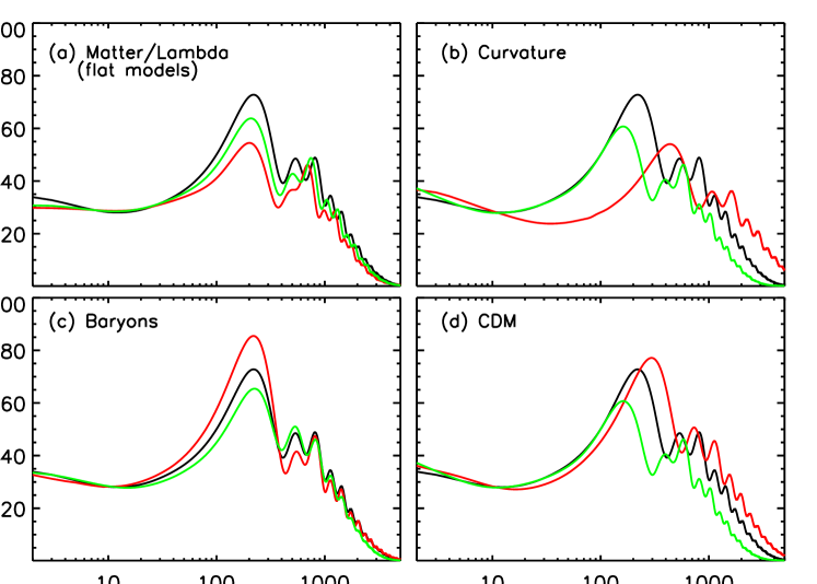
Figure 2: The figure illustrates the sensitivity of the temperature anisotropy to changes in various parameters, about the standard $\Lambda$CDM model of Figure 1. The black (dark) line is always the standard $\Lambda$CDM model. Figure (a): Shows sensitivity to matter/lambda densities for flat models. The three plots with decreasing peak amplitudes result from increasing $\Omega_{m}$ to $0.5$ and $1$, keeping total $\Omega_{T}=1$. Figure (b): Here the effect of total curvature on peak location is illustrated. The plot with the smallest $l$ value for the first peak has $\Omega_{m}=0.448$, $\Omega_{\Lambda}=0.73$, while that with the largest is for an open universe, with $\Omega_{m}=0.27$ and $\Omega_{\Lambda}=0$. Figure (c): Shows the sensitivity to the baryon density. For the three plots with decreasing first peak amplitudes, one has $\Omega_{b}=0.092$, $0.046$ and $0.023$ respectively. Figure (d): The sensitivity to the CDM density parameter. This is $0.112$, $0.224$ and $0.448$ for the three plots, where the first peak progressively shifts to lower $l$ values.

These dependencies are accurate to few percent levels for variation around the WMAP inferred parameters pageetal2003 . WMAP does not yet clearly measure the third peak, but from previous compilations wang03 , Page et al estimate $H_{3}=0.42\pm 0.08$. Note that if $n_{s}$ is fixed, $\omega_{b}$ is well constrained by $H_{2}$ and then $\omega_{m}$ from $H_{3}$. For more details we refer the reader to pageetal2003 . We show in Figure 2 a set of $C_{l}$ versus $l$ curves, generated using CMBFAST, which illustrate the sensitivity of the CMBR to the cosmological parameters discussed above.

VIII.5 Other sources of CMB anisotropies

So far we have concentrated on the primary temperature anisotropies generated at the LSS; a number of effects can generate additional anisotropies after recombination, generally referred to as ’secondary anisotropies’. We do not discuss these in detail; for an extensive review see hudodr . Of the gravitational secondaries, we have already discussed the ISW effect arising from the changing gravitational potential. This effect is also important if there are tensor metric perturbations, say due to stochastic gravitational waves generated during inflation tensorsv . Another important gravitational secondary arises due to gravitational lensing (cf. hudodr and references therein). Scattering effects due to free electrons along the line of sight can also produce a number of effects. The electrons can arise in collapsed objects like clusters or due to re-ionization of the universe. We discuss the effects of re-ionization later below. The scattering of the CMB due to the ionized electrons in clusters of galaxies was first discussed by Sunyaev and Zeldovich (SZ) sun_zel72 . The SZ effect generates power below the damping tail in the $C_{l}$ spectrum, at a level which depends on the normalization of the density power spectrum, $\sigma_{8}$. (Here $\sigma_{8}$ is the RMS density contrast when the density field is smoothed over a ’top hat’ sphere of radius $8h^{-1}\,{\rm Mpc}$). Recently a significant excess power was detected by the CBI experiment cbiobs , at small angular scales ( $l>2000$) at a level of $\sim 355(\mu\,{\rm K})^{2}$. This can arise from the SZ effect, but requires a somewhat large $\sigma_{8}\sim 1$ (cf. cbisz ), larger than values previously assumed. Alternatively the CBI result may point to new physics; it has been suggested for example that primordial magnetic fields can be a significant contributor to the power at large $l$ ksjdb_bc ; trsksjdb . Primordial tangled magnetic fields generate vortical ( Alfvén wave mode) perturbations which lead to temperature anisotropies due to the doppler effect. They also survive Silk damping on much smaller scales compared to the scalar modes jedam ; ksjdba . The test of whether the CBI excess is indeed produced by the SZ effect, will come from the spectral dependence of the excess power (if it is due to the SZ effect, there should be such a spectral dependence), and measurements of polarization on these small angular scales (see below). There are several other interesting gravitational and scattering secondaries which can generate temperature anisotropies, and we refer the interested reader to the excellent review hudodr .

IX Polarization of the CMBR

IX.1 The origin of CMB polarization

It was realized quite soon after the discovery of the CMB that it can get polarized rees68 . Polarization of the CMBR arises due to Thomson scattering of the photons and the electrons, basically because the Thomson cross section is polarization dependent. We used in earlier sections the cross section relevant for unpolarized light, ignoring the small effects of polarization on the temperature evolution. Scattering of radiation which is isotropic or even one which has a dipole asymmetry is however not capable of producing polarization. The incoming radiation needs to have a quadrupole anisotropy. The general features of CMBR polarization are discussed in detail in some excellent reviews kosowsky ; huwhite_new . Note that in the tight coupling limit, the radiation field is isotropic in the fluid rest frame, and can have at most a dipole anisotropy in the frame in which the fluid moves. The quadrupole anisotropy is zero. However to the next order, departures from tight coupling, due to a finite photon mean free path, in the presence of velocity gradients, can generate a small quadrupole anisotropy.

A qualitative argument is as follows zal03 : The last scattering electron (say $O$ at $\bm{x}_{0}$) sees radiation from the ’last but one scattering’ electron ($P$), roughly a photon mean free path ($L_{\gamma}$) away, say at a location $\bm{x}=\bm{x}_{0}+L_{\gamma}\bm{n}$. Here $\bm{n}$ is the direction from $O$ to $P$. The velocity of the baryon-photon fluid at $P$ is $v_{i}(\bm{x})\approx v_{i}(\bm{x}_{0})+L_{\gamma}n_{j}\partial_{j}v_{i}(\bm{x}_{0})$. Due to the Doppler shift, the temperature seen by $O$ is $\delta T(\bm{x}_{0},\bm{n})/T\sim n_{i}[v_{i}(\bm{x})-v_{i}(\bm{x}_{0})]=L_{\gamma}n_{i}n_{j}\partial_{j}v_{i}(\bm{x}_{0})$. This is quadratic in $\bm{n}$ and so corresponds to a quadrupole anisotropy as seen by the last scattering electron. The Thomson scattering of this quadrupole anisotropy can lead to polarization of the CMBR. The fractional polarization anisotropy generated is $\Delta_{P}\sim kL_{\gamma}V$.

One complication is that $L_{\gamma}$ grows rapidly as photons and baryons decouple during recombination. An approximate estimate of its effect, would be to weigh the polarization amplitude derived above, with the probability of last scattering at a given epoch described by the visibility function. Note that the visibility function goes as $\dot{\tau}e^{-\tau}$, where $\dot{\tau}=1/L_{\gamma}$. So during the tight coupling evolution, the $L_{\gamma}$ factor cancels out and after the weighting one gets instead $\Delta_{P}\sim k\delta\eta^{*}V$, where $\delta\eta^{*}$ is the width of the LSS. So the effective photon mean free path generating quadrupole anisotropy and hence polarization of the CMB becomes $\delta\eta^{*}$, the average distance photons travel between their last and last but one scattering, during decoupling. Such an estimate is verified in a more careful calculation zalhar95 .

IX.2 Describing CMBR polarization

There is another complication that has to be handled when dealing with polarization, the fact that polarization is not a scalar quantity. It is conventional to describe polarization in terms of the Stokes parameters, $I$, $Q$, $U$ and $V$, where $I$ is the total intensity, whose perturbed version was called $i$ above, and discussed extensively in earlier sections. For a quasi-monochromatic wave, propagating in the $z$-direction, we can describe the electric field at any point in space as $E_{x}=a_{x}(t)\cos[\omega_{0}t-\theta_{x}(t)]$ and $E_{y}=a_{y}(t)\cos[\omega_{0}t-\theta_{y}(t)]$, where the amplitudes $a_{x}$, $a_{y}$ and the phases $\theta_{x}$, $\theta_{y}$ vary slowly in time, compared to $\omega_{0}^{-1}$. The stokes parameters are defined as the time averages: $I=\langle a_{x}^{2}\rangle+\langle a_{y}^{2}\rangle$, $Q=\langle a_{x}^{2}\rangle-\langle a_{y}^{2}\rangle$, $U=\langle 2a_{x}a_{y}\cos(\theta_{x}-\theta_{y})\rangle$, $V=\langle 2a_{x}a_{y}\sin(\theta_{x}-\theta_{y})\rangle$. Unpolarized light has $Q=U=V=0$. The parameters $Q$ and $U$ describe linear polarization, while $V$ describes circular polarization. At the zeroth order the CMB is unpolarized and its small polarization is expected to arise as explained above due to Thomson scattering. This does not produce circular polarization and so one can set $V=0$.

Note that under a rotation of the $x$ and $y$ axis through an angle $\psi$, the parameters $I$ and $V$ are invariant but $(Q\pm\mathrm{i}U)^{\prime}=e^{\mp 2\mathrm{i}\psi}(Q\pm\mathrm{i}U)$. So $Q\pm\mathrm{i}U$ transform as a spin 2 Tensor under rotation of the co-ordinate axis. The standard spherical harmonics do not provide the appropriate basis for its Fourier expansion on the sky. One then adopts the following approach to this problem zal_sel97 ; KKS97 ; construct scalars under rotation from $Q\pm\mathrm{i}U$ by using spin-lowering ($\partial^{-}$) and spin-raising ($\partial^{+}$) operators, and then make a standard $Y_{lm}$ expansion. Or alternatively construct tensor (’spin’ weighted) spherical harmonics, ${}_{\pm 2}Y_{lm}$ by operating on the $Y_{lm}$’s twice with spin-raising or lowering operators, and then expand

$$(Q\pm\mathrm{i}U)(\bm{n})=\sum_{lm}a_{\pm 2,lm}\ (_{\pm 2}Y_{lm})$$ (73)

in this basis. Alternatively $a_{\pm 2,lm}$ can also be thought of as the $Y_{lm}$ expansion co-efficients of the spin zero quantities, $(\partial^{-})^{2}(Q+\mathrm{i}U)$ and $(\partial^{+})^{2}(Q-\mathrm{i}U)$ respectively, apart from an $l$ dependent normalization factor. The explicit expressions for the raising and lowering operators, the spin weighted harmonics, and the expansions in terms of these are given in zal_sel97 . For example we can write,

$$a_{\pm 2,lm}=\int d\Omega\ (_{\pm 2}Y^{*}_{lm}(\bm{n}))\ (Q\pm\mathrm{i}U)(\bm{n})=\left[\frac{(l+2)!}{(l-2)!}\right]^{-1/2}\int d\Omega\ Y^{*}_{lm}(\bm{n})\left[(\partial^{\mp})^{2}(Q\pm\mathrm{i}U)(\bm{n})\right]$$ (74)

Since $a_{\pm 2,lm}$ are expansion co-efficients of scalar quantities under rotation, they can be used to characterize the polarization on the sky in an ’invariant’ manner. More convenient is to use the linear combinations, $a_{E,lm}=-(a_{2,lm}+a_{-2,lm})/2$ and $a_{B,lm}=\mathrm{i}(a_{2,lm}-a_{-2,lm})/2$ zal_sel97 ; new_pen66 , and the associated real space polarization fields; $E(\bm{n})=\sum_{lm}a_{E,lm}Y_{lm}(\bm{n})$ and $B(\bm{n})=\sum_{lm}a_{B,lm}Y_{lm}(\bm{n})$. The $E$ and $B$ fields specify the polarization field ($Q$ and $U$) completely, are invariant under rotation (just like the temperature $\Theta(n)$) and have definite parity. Under a parity transformation, $E$ remains invariant while $B$ changes sign new_pen66 . The convenience of the $E$-$B$ split comes from the fact that scalar perturbations do not produce any $B$ type polarization. An alternative way of thinking about the $E$ and $B$ split is that they are the gradient and curl type components of the polarization tensor KKS97 . More details of these fascinating but somewhat complicated ideas can be got from the two seminal papers on the subject KKS97 ; zal_sel97 .

In order to describe the statistics of CMBR anisotropies fully, including its polarization, we have to now consider not only $C_{l}$ due to the temperature anisotropy $\Theta$, but also corresponding power spectra of $E$, $B$ and the cross correlation between $\theta$ and $E$. Note that the cross correlation between $B$ and $\Theta$, and $B$ and $E$ vanish if there are no parity violating effects. Since $E$ and $B$ are rotationally invariant quantities, we can define the power spectra $C_{l}^{E}$, $C_{l}^{B}$ and $C_{l}^{TE}$ in an analogous way to the temperature power spectrum. We now turn to their computation.

IX.3 Computing the polarization power spectrum

We focus on scalar perturbations. In this case for any given Fourier mode $\bm{k}$, one can define a co-ordinate system with $\bm{k}\parallel\hat{\bf z}$, and for each plane wave, treat the Thomson scattering as the radiative transport through a plane parallel medium. It turns out that only Stokes Q is generated in this frame because of azimuthal symmetry, and its amplitude depends only on $\mu=\bm{n}\cdot\hat{\bm{k}}$. The stokes parameter $U=0$ in this frame, for each $\bm{k}$ mode. Because $U=0$ and $Q$ is only a function of $\mu$, one has $(\partial^{-})^{2}(Q+\mathrm{i}U)=(\partial^{+})^{2}(Q-\mathrm{i}U)$. (From the explicit form of the spin-raising/lowering operators give in zal_sel97 , it can be checked that $(\partial^{-})^{2}(f(\mu))=(\partial^{+})^{2}(f(\mu))$ for any azimuthally symmetric function which depends only on $\mu$. Second since $U=0$, we have $(Q+\mathrm{i}U)=(Q-\mathrm{i}U)$). Therefore $a_{2,lm}=a_{-2,lm}$, and we have $a_{B,lm}=0$ for such scalar perturbations.

The Boltzmann equation including polarization is given by a number of authors (see for example bond_efs84 ; ma_bert ; hu_white97 ). We will simply quote the result, got using the detailed treatment by hu_white97 . We have

$$C_{l}^{E}=\frac{2}{\pi}\int{dk\over k}k^{3}\langle|a_{l}^{E}(k,\eta_{0})|^{2}\rangle;\qquad a_{l}^{E}(k,\eta_{0})=-\int d\eta\ g(\eta_{0},\eta)\frac{kL_{\gamma}V}{3}\left[\frac{(l+2)!}{(l-2)!}\right]^{1/2}\frac{j_{l}(k\Delta\eta)}{(k\Delta\eta)^{2}}$$ (75)

where we have expressed the quadrupole source for the polarization anisotropy, $P=(\Theta_{2}-\sqrt{6}E_{2})/10$, by its tight coupling limit $P=2kL_{\gamma}V/9$ (see hu_white97 ). As argued on qualitative grounds above, polarization is sourced by the velocity differences of the fluid, over a photon mean free path (i.e. $kVL_{\gamma}$). Once again the spherical Bessel function $j_{l}(k\Delta\eta)$ in Eq. (75) will at a given $l$, pick out (on $k$ integration) a scale $k\sim l/\Delta\eta$ at around last scattering, while the visibility function $g$ weighs the contribution at any time $\eta$ by the probability of last scattering from that epoch.

Suppose we wish to estimate the polarization anisotropy on physical scales much bigger than the thickness of the last scattering surface, or $l\sim kR^{*}<1000$ or so. As we explained earlier, the visibility function goes as $\dot{\tau}e^{-\tau}$ whereas the polarization source is $kL_{\gamma}V/3=(kV/3)(\dot{\tau})^{-1}$, and so in their product, $\dot{\tau}$ cancels and only $e^{-\tau}(kV/3)$ would survive. The integral over $\eta$ in Eq. (75), would be nonzero only for a range of epochs of order the width $\delta\eta^{*}$ of the LSS. (Note that just after recombination, the tight coupling expression cannot be used; however there is also no polarization for $\eta>\eta^{*}$ because there is negligible further Thomson scattering). So one expects a contribution of order $kV\delta\eta^{*}/3$ in doing this integral, apart from an evaluation of the other terms at $\eta^{*}$. A more rigorous analysis, following the time evolution of the polarization source term, gives a further factor of $\sim 1/2$ reduction, if $\delta\eta^{*}$, is defined as the Gaussian width of the visibility function zalhar95 . Making such an approximation, and putting in the tight coupling expression for the velocity of the photon-baryon fluid, gives

$$a_{l}^{E}(k,\eta_{0})=-\frac{k\delta\eta^{*}}{6}\ \Phi_{0}\ E(k)(1+3R)c_{s}\sin k\eta_{s}^{*}\left(\frac{l}{kR^{*}}\right)^{2}\ j_{l}(kR^{*})$$ (76)

Note that again the $k$ integral to find $C_{l}^{E}$ will pick out values of $kR^{*}\sim l$. We can infer a number of features of the polarization from the above:

• The magnitude of the polarization anisotropy, is of order $\Delta P\sim 0.6(k\delta\eta^{*})(\Phi_{0}/3)=0.6\ l(\delta\eta^{*}/R^{*})(\Phi_{0}/3)$, where we have taken $R\sim 0.6$. Adopting $\delta\eta^{*}\sim 10h^{-1}\,{\rm Mpc}$ and $R^{*}\sim 10^{4}h^{-1}\,{\rm Mpc}$, we get at $l\sim 100$, a polarization anisotropy about $6\%$ of the Sachs-Wolfe contribution (or about $2\mu\,{\rm K}$). The amplitude rises with $l$, but at large $l>l_{D}$ the Silk damping cuts off the baryon-photon velocity, and so the polarization gets cut off as $e^{-(l/l_{D})^{m}}$, say. This gives a maximum contribution at $l<l_{D}$ depending on the $m$, with peak amplitude of order $10\%$ of the peak temperature anisotropies. These order of magnitude estimates are borne out by the more detailed numerical integration using CMBFAST shown in Figure 1.

• The acoustic oscillations of the baryon-photon fluid velocity imprints such oscillations also on the polarization. The polarization will display peaks when $\sin(kr_{s}^{*})=\pm 1$, or for $kr_{s}^{*}=(2n+1)(\pi/2)$, with $n=0,1,..$, corresponding to $l\sim(2n+1)l_{A}/2$. These peaks are out of phase with the temperature acoustic peaks, as they arise due to the velocity, and they are sharper (since for temperature there is a partial filling in of the troughs by the velocity contribution).

• Both the polarization and the temperature depend on the potential $\Phi$, and so one expects a significant cross correlation power $C_{l}^{TE}$. Further, the $j_{l}$ term does not significantly correlate with $j_{l}^{\prime}$ term in the $k$-integral for $C_{l}^{TE}$. So this cross correlation will be dominated by the product of the temperature monopole with a $\cos(kr_{s}^{*})$ dependence and the polarization (of $E$ type) with a $\sin(kr_{s}^{*})$ dependence. The peaks of $C_{l}^{TE}$ will then occur when $\sin(kr_{s}^{*})\cos(kr_{s}^{*})\propto\sin(2kr_{s}^{*})=\pm 1$, or when $kr_{s}^{*}=(2n+1)(\pi/4)$, with $n=0,1,..$, corresponding to $l\sim(2n+1)l_{A}/4$. So $C_{l}^{TE}$ has oscillations at twice the frequency compared to the temperature or polarization. There will be shifts in the exact location of the $C_{l}^{E}$ and $C_{l}^{TE}$ peaks, as for the temperature.

• The $E$ type polarization has been detected at a $5\sigma$ level by the Degree Angular scale Interferometer (DASI) at $l$ values of a few hundred, and at a level consistent with the expectations from the detected temperature anisotropy kovac02 . The CBI experiment has also detected the $E$ type polarization, with the peaks in the polarization spectrum showing the expected phase shifts compared to the peaks of the temperature spectrum read2 . The $TE$ cross correlation was detected at $95\%$ significance by DASI, but there is no evidence of any $B$ type polarization. The cross correlation has also been detected by WMAP. The WMAP experiment has released results on $C_{l}^{TE}$, although not on $C_{l}^{E}$. WMAP detects significant negative $C_{l}^{TE}$, at $l\sim 150$ and a positive ’peak’ at $l\sim 300$. The existence of such an anti-correlation between temperature and polarization is an indication that there exist ’super-Hubble’ scale fluctuations on the LSS. This is interpreted as strong evidence for inflation type models, since models which involve seeds (like cosmic strings) can produce super Hubble scale temperature fluctuations (due the ISW type effects) but not the observed anti-correlation in $C_{l}^{TE}$.

IX.4 $B$ type polarization

So far we have emphasized the $E$ type polarization, as scalar modes do not produce the $B$ type signal. However models of inflation which are thought to generate the scalar perturbations, can also generate a stochastic background of gravitational waves. These tensor perturbations and the CMBR anisotropy that they generate has also been studied in detail tensors , although we will not do so here. Their effects are best separated from the scalar mode signals, by the fact that Tensors also lead to $B$ type polarization anisotropy zal_sel97 ; KKS97 . The temperature contribution from tensors is flat roughly upto $l\sim 100$ after which it rapidly falls off. The polarization contribution, produced at recombination, peaks at $l\sim 100$. The peak amplitude of the signal is however expected to be quite small in general with $(l(l+1)C_{l}^{B}/2\pi)^{1/2}\sim 0.1\mu\,{\rm K}(E_{inf}/2\times 10^{16}{\rm GeV})^{2}$, where $E_{inf}$ is the energy scale of inflation. zal03 . (An $E_{inf}\sim 2\times 10^{16}{\rm GeV}$ corresponds to the ratio of the $l=2$ contribution due to tensors compared to scalar, $T/S\approx 0.1$). One of the prime motivations for measuring polarization with great sensitivity is to try and detect the contribution from stochastic gravitational waves. The $B$ type anisotropy can also arise due to gravitational lensing of the CMB, even if one had only $E$ type polarization arising from the recombination epoch zal_sel98b . This could set the ultimate limitation for detecting the $B$ mode from gravity waves. Another interesting source for $B$ type polarization are vector modes, arising perhaps due to tangled magnetic fields generated in the early universe trsksjdb ; seshksjdb ; mack ; lewis , or even present in the initial conditions lewisb . Indeed if there were helical primordial magnetic fields, at the LSS, parity invariance can be broken and one can even generate $T-B$ cross correlations dur_tan .

IX.5 Reionization and CMBR polarization

One of the surprises in the WMAP results was the detection of a significant excess cross-correlation power $C_{l}^{TE}$ at low $l$, over and above that expected if polarization was only generated at recombination. This can be interpreted as due to the effects of re-ionization, But one seems to need a significantly higher optical depth to the re-ionized electrons $\tau_{ri}\sim 0.17$, and a correspondingly high redshift for reionization $z_{ri}\sim 17$. The probes and models of the high redshift intergalactic medium, including the use of the CMBR as a probe of re-ionization is discussed more fully elsewhere in this volume by Sethi sethi04 . We make a few qualitative remarks.

First, note that if photons are re scattered, due to electrons produced in re-ionization, the visibility function will have 2 peaks; one narrow peak around recombination, and a broader peak around the re-ionization epoch (cf. Figure 2 in sethi04 ), which depends on the exact re-ionization history. The probability for last scattering around the usual LSS will diminish by a multiplicative factor $e^{-\tau_{ri}}$, where $\tau_{ri}$ is the optical depth for electron scattering to the re-ionization epoch. At the same time new temperature and polarization anisotropies get generated. The most important effect is that Thomson scattering by electrons generated during re-ionization, produces additional polarization. Note that the quadrupole anisotropy at the the re-ionization epoch is likely to be much larger than at recombination, simply because the monopole can free stream to generate a significant quadrupole at the new LSS. At re-ionization redshifts close enough to the observer, the relevant monopole becomes the Sachs-Wolfe value $\Theta_{0}+\Phi=\Phi_{0}/3$. The quadrupole at the re-ionized epoch $\eta_{ri}$ can then be simply estimated by replacing $\eta_{0}$ in Eq. (37), by $\eta_{ri}$. One gets $\Theta_{2}(\bm{k},\eta_{ri})=a_{2}(\bm{k},\eta_{ri})=(\Phi_{0}/3)j_{2}(k(\eta_{ri}-\eta^{*}))$. Note that this does not have the $kL_{\gamma}$ suppression factor, which obtains around recombination. Also $E_{2}$ in the polarization source term $P$ above is negligible. In evaluating the $E$ type polarization arising from the re-ionization, one can substitute the resulting $P=\Theta_{2}/10$ in Eq. (75) instead of $P=2kL_{\gamma}V/9$; for the range of $\eta$ where scattering by electrons generated due to re-ionization is important.

The resulting re-ionization contribution can be best calculated numerically, for example using CMBFAST, as illustrated by Sethi (this volume). But the scale where the peak in the power spectra can be estimated noting that $a_{l}^{E}$ will involve the product $j_{2}(k(\eta_{ri}-\eta^{*}))j_{l}(k(\eta_{0}-\eta_{ri}))$, which contributes to the $k$-integral dominantly when both $k(\eta_{ri}-\eta^{*})\sim 2$ and $k(\eta_{0}-\eta_{ri})\sim l$. This implies that the re-ionization contribution to $E$ type polarization peaks at $l\sim 2(\eta_{0}-\eta_{ri})/(\eta_{ri}-\eta^{*})\sim 10$ for the parameters appropriate for a $\Lambda$CDM cosmology and a $z_{ri}\sim 20$. This scale basically reflects the angle subtended by the Hubble radius at re-ionization. One has to also take account of the damping due to the large width of the LSS at re-ionization, which will shift the peak to smaller $l$.

The $k$ integral which determines $C_{l}^{TE}$, involves the product $j_{2}(k(\eta_{ri}-\eta^{*}))j_{l}(k(\eta_{0}-\eta_{ri}))j_{l}(kR^{*})$, the last $j_{l}(kR^{*})$ coming from the temperature contribution from the usual LSS. Note that $\eta_{0}$ is much bigger than both $\eta_{ri}$ and $\eta^{*}$, and the two $j_{l}$ factors will re-inforce each other for small $l$. The cross correlation peak will occur at an $l$ similar to the peak in $C_{l}^{E}$. The indication from the WMAP data for significant optical depth from re-ionization is not easy to explain (cf. reiond ). If the preliminary WMAP result continues to firm up with subsequent years data, it will set very strong constraints on the star and active galaxy formation at high redshift. It may be also worth exploring new physical alternatives. For example Ref sethi_sub , explores the possibility that tangled magnetic fields generated in the early universe could form subgalatic objects at high enough redshifts to impact significantly on re-ionization. Note that if there is significant optical depth to re-ionization, then inhomogeneities at the new LSS can lead to new secondary sources of both temperature ostriker_vish and polarization anisotropies polin . Eventually the detailed measurement of the polarization signals, could be a very effective probe of the reionization history of the universe kaplin .

X Concluding remarks

In this review we have tried to emphasize the physics behind the generation of CMBR anisotropies. We have given details of the computation of the primary temperature anisotropies, and also indicated the relevant issues for polarization. Our aim is more to introduce the budding cosmologist to the well known (and reviewed) techniques used to calculate the CMB anisotropies, rather than provide an extensive survey of observations and results. Of course, it is the existence of very good observational data that makes the effort worthwhile. Clearly the CMB is and will continue to be a major tool to probe structure formation and cosmology. We have already learned a great deal from the detailed observations of the degree and sub degree scale temperature anisotropies, particularly the acoustic peaks. The exploration of small angular scale anisotropies is just at a beginning stage and holds the promise of revealing a wealth of information, on the gastrophysics of structure formation. The future lies in also studying in detail the polarization of the CMBR. Already WMAP results have revealed a surprisingly large redshift for the re-ionization of the universe. Polarization will also be a crucial probe of the presence of gravitational waves. We can expect in the years to come much more information on cosmology from WMAP, future missions like PLANK and other CMB experiments, with the possibility of more surprises!

Appendix A The collision term: details

Consider the integral over the collision term on the RHS of Eq. (25). We have $\int p^{3}dp\bar{c}(f)=n_{e}\sigma_{T}(A_{1}+A_{2})$ where

$$A_{1}=\int p^{3}dp{d\Omega^{\prime}\over 4\pi}[\bar{f}(\bar{p},\bar{\bf n}^{\prime})-\bar{f}(\bar{p},\bar{\bf n})];\quad A_{2}=\int p^{3}dp{d\Omega^{\prime}\over 4\pi}{1\over 2}P_{2}(\bar{\bf n}\cdot\bar{\bf n}^{\prime})[\bar{f}(\bar{p},\bar{\bf n}^{\prime})-\bar{f}(\bar{p},\bar{\bf n})]$$ (77)

are respectively, the isotropic and anisotropic contribution to the collision term. From the invariance of the scalar $p_{i}u^{i}$, where $u^{i}$ is the four velocity corresponding to the bulk motion of the electron (Baryonic) fluid we can show that

$$p=a(1+{\bf n}.{\bf v})(1-\phi)\bar{p}$$ (78)

(We have used here the fact that in the fluid rest frame the components of $\bar{u}^{i}=(1,0,0,0)$, while $u^{i}=(\gamma_{v}/\sqrt{g_{00}},\gamma_{v}\bm{v}/\sqrt{|g_{\beta,\beta}|})$ with $\gamma_{v}=(1-v^{2}/c^{2})^{-1/2}$). We split $A_{1}=I_{1}-I_{2}$ with

$$I_{1}=\int p^{3}dp{d\Omega^{\prime}\over 4\pi}\bar{f}(\bar{p},\bar{\bf n}^{\prime})\quad I_{2}=\int p^{3}dp{d\Omega^{\prime}\over 4\pi}\bar{f}(\bar{p},\bar{\bf n})]$$ (79)

For evaluating $I_{2}$ we use the fact that $f$ is a scalar, that is $\bar{f}(\bar{p},\bar{\bf n})=f(p,{\bf n})$. Also the integrand of $I_{2}$ does not depend on $\bar{\bf n^{\prime}}$. So we have $I_{2}=\int p^{3}dpf(p,{\bf n})=(\rho_{R}a^{4}/4\pi)[1+i]$. For evaluating $I_{1}$ we stay in the initial electron rest frame and transform the integral over $p$ to one over $\bar{p}$ using Eq. (78). We get $I_{1}=(a^{4}/4\pi)(1-4\phi)(1+4{\bf n}\cdot{\bf v})\bar{\rho}$ where we have used the fact that $\bar{\rho}=\int d^{3}\bar{\bf p}\bar{p}\bar{f}(\bar{\bf p})$ is the energy density of radiation in the fluid rest frame. Using the invariance of $T^{i}_{k}u_{i}u^{k}$, and from the fact that the components of both $u^{i}$ and $T^{i}_{k}$ which involve one spatial index are of order $v/c$, we can check that $\bar{\rho}=\rho+O(v^{2}/c^{2})$. Since, $\rho=\rho_{R}(1+4\phi)(1+i_{0})$, to linear order $I_{1}=(a^{4}\rho_{R}/4\pi)(1+4{\bf n}\cdot{\bf v}+i_{0})$. So

$$A_{1}={a^{4}\over 4\pi}\rho_{R}\left[i_{0}+4\bm{n}\cdot\bm{v}-i\right]$$ (80)

To simplify $A_{2}$, we use the addition theorem for spherical harmonics to write

$$A_{2}=\sum_{m=-2}^{2}\frac{Y_{2m}(\bar{\bm{n}})}{10}\int p^{3}dp\ d\Omega^{\prime}\ Y_{2m}^{*}(\bar{\bm{n}}^{\prime})[\bar{f}(\bar{p},\bar{\bm{n}}^{\prime})-\bar{f}(\bar{p},\bar{\bm{n}})]={a^{4}\rho_{R}\over 4\pi}\frac{1}{10}\sum_{m}[Y_{2m}(\bm{n})i_{2m}],$$ (81)

where $i_{2m}=\int d\Omega Y^{*}_{2m}i(\bm{x},\eta,\bm{n})$. In evaluating $A_{2}$ we have used the fact that the term $\bar{f}(\bar{p},\bar{\bm{n}})$ does not contribute to the integral over $d\Omega^{\prime}$. Also writing $\bar{f}(\bar{p},\bar{\bm{n}}^{\prime})=f(p,\bm{n}^{\prime})=f_{b}(p)+f_{1}(p,\bm{n}^{\prime})$, the $f_{b}$ term gives zero contribution. And since $f_{1}$ is already first order in perturbations, we can evaluate $A_{2}$ by replacing $\bar{\bm{n}}$ and $\bar{\bm{n}}^{\prime}$ by their unbarred values (these will differ only by terms of order $v/c$ and the difference when multiplied by $i_{2m}$ will not contribute to the first order).

Finally, we also need to evaluate $d\tau/d\eta$. Since $A_{1}$ and $A_{2}$ are already of first order, we need to evaluate this term only to zero’th order, to write down the equation for the perturbed brightness. We have $d\tau/d\eta=\bar{u}^{0}/u^{0}=a$ to the leading order. The perturbed brightness equation (26), given in the main text, is got from Eq. (25), Eq. (80) and Eq. (81).

Appendix B Silk damping: details

We have given in the main text the iterative solution to Eq. (45) to the first order in $L_{\gamma}$. To derive Silk damping one needs to go to the second order iteration,

$$i^{(2)} = i^{(0)}-L_{\gamma}\left[\frac{\partial i^{(1)}}{\partial\eta}+\bm{n}\cdot\bm{\nabla}i^{(1)}+8\bm{n}\cdot\bm{\nabla}\phi\right]$$ (82)

$$= i^{(1)}+L_{\gamma}^{2}\left[\frac{\partial}{\partial\eta}+\bm{n}\cdot\bm{\nabla}\right]\left[\frac{\partial i^{(0)}}{\partial\eta}+\bm{n}\cdot\bm{\nabla}i^{(0)}+8\bm{n}\cdot\bm{\nabla}\phi\right]$$

As mentioned in the text, we neglect the anisotropy of the Thomson scattering, and also the effects of the gravitational potential $\phi$. Taking the zeroth moment of Eq. (82) , we get

$$i_{0}=i_{0}-L_{\gamma}\left[\frac{\partial i_{0}}{\partial\eta}+\frac{4}{3}\bm{\nabla}\cdot\bm{v}\right]+L_{\gamma}^{2}\left[\frac{\partial^{2}i_{0}}{\partial\eta^{2}}+\frac{8}{3}\frac{\partial(\bm{\nabla}\cdot\bm{v})}{\partial\eta}+\frac{1}{3}\bm{\nabla}^{2}i_{0}\right]$$ (83)

So to the next order in $L_{\gamma}$, Eq. (49) is modified to

$$\frac{\partial i_{0}}{\partial\eta}+\frac{4}{3}\bm{\nabla}\cdot\bm{v}=L_{\gamma}\left[\frac{4}{3}\frac{\partial(\bm{\nabla}\cdot\bm{v})}{\partial\eta}+\frac{1}{3}\bm{\nabla}^{2}i_{0}\right]$$ (84)

Similarly, taking the first moment of Eq. (82) the Euler equation Eq. (52) gets modified to

$$\left[\rho_{B}+\frac{4}{3}\rho_{R}\right]\frac{\partial\bm{v}}{\partial\eta}=-\bm{\nabla}\left(\frac{\rho_{R}i_{0}}{3}\right)+\rho_{R}L_{\gamma}\left[\frac{4}{3}\frac{\partial^{2}\bm{v}}{\partial\eta^{2}}+\frac{2}{3}\bm{\nabla}\left(\frac{\partial i_{0}}{\partial\eta}\right)+\frac{8}{15}\bm{\nabla}(\bm{\nabla}\cdot\bm{v})+\frac{4}{15}\bm{\nabla}^{2}\bm{v}\right]$$ (85)

Here we have used the relation $\int(d\Omega/4\pi)n_{i}n_{j}n_{k}n_{l}=[\delta_{ij}\delta_{kl}+\delta_{ik}\delta_{jl}+\delta_{il}\delta_{kj}]/15$. (This can be written down from symmetry and the coefficients and its amplitude fixed by contracting over any two indices). We have also neglected the baryonic pressure compared to the radiation pressure. Equations (84) and (85) form a pair of linear coupled equations for the the perturbations in radiation density $i_{0}$ and matter velocity $\bm{v}$. Assuming that the rate of variation of of the co-efficients of various terms, due to Hubble expansion is small (compared to $kc_{s}$), one can use the WKBJ approximation, to derive the dispersion relation for the baryon-radiation acoustic oscillations.

Consider therefore a plane wave solution of the form

$$\bm{v}=\bm{V}\exp(\mathrm{i}\bm{k}\cdot\bm{x}+\int\Gamma d\eta);\quad i=I\exp(\mathrm{i}\bm{k}\cdot\bm{x}+\int\Gamma d\eta)$$ (86)

Let us also look at longitudinal waves with $\bm{k}$ parallel to $\bm{V}$. Infact, taking the divergence of Eq. (85) one can see that these modes are completely decoupled from the rotational modes. To leading order one gets from Eq. (84) and Eq. (85), a dispersion relation which is a cubic equation for $\Gamma$,

$$-L_{\gamma}\Gamma^{3}+b\Gamma^{2}+b\Gamma\frac{k^{2}L_{\gamma}}{3}\left[1-\frac{6}{5b}\right]+\frac{k^{2}}{3}=0$$ (87)

which can be solved iteratively. Here we have defined $b=(1+3\rho_{B}/4\rho_{R})=1+R$. To the lowest order we get $\Gamma=\pm i(k/\sqrt{3b})$. So to the zeroth order the dispersion relation is that of a sound (pressure) wave in the baryon-photon fluid, with an effective sound speed $c_{s}=(1/\sqrt{3b})$. Consider the effects of terms proportional to $L_{\gamma}$. Since the $\Gamma^{3}$ term is already multiplied by $L_{\gamma}$ we can use the lowest order solution to write $-L_{\gamma}\Gamma^{3}=-L_{\gamma}(-k^{2}/3b)\Gamma$. This reduces the cubic equation to the quadratic equation

$$\Gamma^{2}+\Gamma\frac{k^{2}L_{\gamma}}{3}\left[1-\frac{6}{5b}+\frac{1}{b^{2}}\right]+\frac{k^{2}}{3b}=0$$ (88)

whose solution to first order in $L_{\gamma}$ is Eq. (61) given in the main text.

References

- (1) A.A. Penzias, R.W. Wilson, Astrophys. J. 142, 419 (1965)
- (2) J.C. Mather et al, Astrophys. J. 420, 439 (1994); Astrophys.J. 512, 511 (1999).
- (3) D. J. Fixsen et al., Astrophys. J. 473, 576 (1996)
- (4) R.K. Sachs, A.M. Wolfe, Astrophys. J. 147, 73 (1967)
- (5) G.F. Smoot et al, Astrophys. J. Lett. 396, 1 (1992)
- (6) G. Efstathiou, J. R. Bond, S. D. M. White, MNRAS, 258, 1P, (1992).
- (7) T. Padmanabhan, D. Narasimha, MNRAS, 259, 41P (1992).
- (8) J.R. Bond, C.R. Contaldi, D. Pogosyan, Phil. Trans. Roy. Soc. Lond. A, 361, 2435 (2003)
- (9) C.L. Bennett et al, Astrophys. J. Suppl. 148, 1 (2003)
- (10) D.N. Spergel et al, Astrophys. J. Suppl. 148, 175 (2003)
- (11) Seljak, U et al., 2004, astro-ph/0407372 (submitted to PRD)
- (12) M. Tegmark et al, Phys. Rev. D 69, 103501 (2004)
- (13) A. Challinor, Lecture notes. Proceedings of the 2nd Aegean Summer School on the Early Universe (Springer LNP), 22-30 September 2003 (astro-ph/0403344)
- (14) W. Hu, S. Dodelson, Ann. Rev. Astr. Astrophys., 40 , 171 (2002);
- (15) Hu, W., 2003, Annals Phys., 303, 203.
- (16) M. Zaldarriaga, Measuring and Modeling the Universe, from the Carnegie Observatories Centennial Symposia. Cambridge University Press, as part of the Carnegie Observatories Astrophysics Series. Edited by W. L. Freedman, p. 310 (2004) (astro-ph/0305272)
- (17) T. Padmanabhan, Theoretical Astrophysics Volume III: Galaxies and Cosmology, Cambridge University Press, (2002).
- (18) S. Dodelson, Modern Cosmology, Academic Press (2003).
- (19) Seljak, U., and Zaldarriaga, M., 1996 ApJ, 469, 437 Zaldarriaga, and U. Seljak, 1998, Phys. Rev. D., 58, 023003. Zaldarriaga, M., Seljak, U., and Bertschinger, E., 1998 ApJ, 494, 491 Zaldarriaga, M., and Seljak, U., 2000 ApJS, 129, 431.
- (20) V. F. Mukhanov, H. A. Feldman, R. H. Brandenberger, Physics Reports, 215, 203 (1992)
- (21) L. Verde et al., Astrophys. J. Suppl. 148, 195 (2003)
- (22) Bucher, M., Moodley, K. and Turok, N., 2000, PRD, 62, 083508; Bucher, M. et al., 2004, preprint, astro-ph/0401417.
- (23) Boughn, S. and Crittenden, R., 2004, Nature, 427, 45; Fosalba, P., Gaztanaga, E. and castander, F. J., 2003, ApJ Lett., 597, L89; Nolta, M. R. et al., 2003, astro-ph/0305097.
- (24) W. Hu, and N. Sugiyama, Ap.J., 444, 489 (1995).
- (25) W. Hu, N. Sugiyama, J. Silk, Nature, 386, 37 (1997)
- (26) J. Silk, Astrophys. J., 151, 431 (1968)
- (27) N. Kaiser, Mon. Not. R. Astr. Soc, 202, 1169 (1983)
- (28) W. Hu and M. White, Phys.Rev. D56, 596 (1997).
- (29) P. J. E. Peebles, J. T. Yu, Astrophys. J., 162, 815 (1970)
- (30) R. A. Sunyaev, Ya. B. Zeldovich, Astrophys. Space Science, 7, 3 (1970)
- (31) W. Hu, M. Fukugita, M. Zaldarriaga, M. Tegmark, Astrophys. J., 549, 669 (2001)
- (32) W. Hu, M. White. Astrophys. J., 479, 568 (1997)
- (33) L. Page et al., Astrophys. J. Suppl. 148, 233 (2003)
- (34) Sahni, V, 1990, PRD, 42, 453
- (35) Sunyaev, R. A. and Zeldovich, Y. B., 1972, Comm. Astrophys. Space Phys., 4, 173.
- (36) Mason, B. S. et al., 2003, ApJ, 591, 540. Readhead, A. C. S. et al., 2004, 609, 498.
- (37) Komatsu E., Seljak U., 2002, MNRAS, 336, 1256. Bond J. R, et al., 2002, ApJ, in press (astro-ph/0205386)
- (38) Subramanian K. and Barrow J. D., 1998, PRL, 81, 3575; Subramanian K. and Barrow J. D., 2002, MNRAS, 335, L57
- (39) Subramanian K., Seshadri, T. R. and Barrow J. D., 2003, MNRAS, 344, L31.
- (40) Jedamzik K., Katalinic V. and Olinto A., 1998, PRD, 57, 3264.
- (41) Subramanian K. and Barrow J. D., 1998, PRD, 58, 083502.
- (42) Bond, J. R., Efstathiou, G. and Tegmark, T., 1997, MNRAS, 291, L33.
- (43) Zaldarriaga, M, Spergel, D. and Seljak, U., 1997, ApJ, 488, 1.
- (44) Efstathiou, G. and Bond, J. R., 1999, MNRAS, 304, 75.
- (45) Wang, L., Tegmark, M., Jain, B. and Zaldarriaga, M., 2003, PRD, 68, 123001.
- (46) Rees, M. J., 1968, ApJ, 153, L1.
- (47) Kosowsky, A., 199, Annals Phys., 246, 49.
- (48) Hu, W., and White, M., 1997, New Astronomy, 2, 323.
- (49) Zaldarriaga, M. and Harari, D. D., 1995, PRD, 52, 3276.
- (50) Zaldarriaga, M and Seljak, U., 1997, PRD, 55, 1830.
- (51) Kamionkowski, M., Kosowsky, A. and Stebbins, A., 1997, PRD, 55, 7368.
- (52) Newman, E. and Penrose, R., 1966, J. Maths. Phys., 7, 863.
- (53) Kovac, J. M. et al., 2002, Nature, 420, 772.
- (54) Readhead, A. C. S. et al., 2004, Science, 306, 836.
- (55) Bond, J. R. and Efstathiou, G., 1984, ApJ, 285, L45.
- (56) Ma, C. P. and Bertschinger, E., 1995, ApJ, 455, 7.
- (57) Polnarev, A. G., 1985, Soviet Astron., 62, 1041; Souradeep, T and Sahni, V., 1992, Mod. Phys. Lett. A7, 3541; Crittenden, R. G., Coulson, D. and Turok, N., 1995, PRD, 52, 5402.
- (58) Zaldarriaga, M and Seljak, U. 1998, PRD, 58, 23003.
- (59) Seshadri T. R. and Subramanian K., 2001, PRL, 87, 101301.
- (60) Mack A., Kashniashvili T. and Kosowsky A., 2002, PRD, 65, 123004.
- (61) Lewis, A, 2004, PRD in Press (astro-ph/0406096);
- (62) Lewis, A, 2004, PRD, 70, 043518.
- (63) Pogosian, L., Vachaspati, T. and Winitzki, S., 2002, PRD, 65, 083502; Caprini, C., Durrer, R. and Kahniashvili, T., 2004, PRD, 69, 063006.
- (64) Sethi, S., 2004, Current Science (this volume).
- (65) Fukugita, M. and Kawasaki, M, 2003, MNRAS, 343, L25; Ricotti, M. and Ostriker, J. P., 2004, MNRAS, 352, 547; Madau, P. et al., 2004, ApJ, 604, 484.
- (66) Sethi, S. and Subramanian, K., 2004, (MNRAS in Press), astro-ph/0405413.
- (67) Ostriker, J. P. and Vishniac, E. T., 1986, ApJ Lett., 306, L51; Vishniac, E. T., 1987, ApJ, 322, 597.
- (68) Seshadri, T. R. and Subramanian, K., 1998, PRD, 58, 063002; Weller, J., 1999, ApJ, 527, L1; Hu, W., 2000, ApJ, 529, 12.
- (69) Kaplinghat, M. et al., 2003, ApJ, 583, 24; Holder, G. et al., 2003, ApJ, 595, 13.