Probing the Light Speed Anisotropy with respect to the Cosmic Microwave Background Radiation Dipole

V.G.Gurzadyan^1,2, J.-P.Bocquet³, A.Kashin¹, A.Margarian¹, O. Bartalini ⁴, V. Bellini ⁵, M. Castoldi ⁶, A. D’Angelo ⁴, J.-P. Didelez ⁷, R. Di Salvo ⁴, A. Fantini ⁴, G. Gervino ⁸, F. Ghio ⁹, B. Girolami ⁹, A. Giusa ⁵, M. Guidal ⁷, E. Hourany ⁷, S. Knyazyan ¹, V. Kouznetsov ¹⁰, R. Kunne ⁷, A. Lapik ¹⁰, P. Levi Sandri ¹¹, A. Lleres ³, S. Mehrabyan ¹, D. Moricciani ⁴, V. Nedorezov ¹⁰, C. Perrin ³, D. Rebreyend ³, G. Russo ⁵, N. Rudnev ¹⁰, C. Schaerf ⁴, M.-L. Sperduto ⁵, M.-C. Sutera ⁵, A. Turinge ¹²

¹ Yerevan Physics Institute, 375036 Yerevan, Armenia
² ICRA, Dipartimento di Fisica, Università “La Sapienza", 00185 Roma, Italy
³ IN2P3, Laboratory for Subatomic Physics and Cosmology, 38026 Grenoble, France
⁴ INFN sezione di Roma II and Università “Tor Vergata", 00133 Roma, Italy
⁵ INFN sezione di Catania and Università di Catania, 95100 Catania, Italy
⁶ INFN sezione di Genova and Università di Genova, 16146 Genova, Italy
⁷ IN2P3, Institut de Physique Nucléaire, 91406 Orsay, France
⁸ INFN sezione di Torino and Università di Torino, 10125 Torino, Italy
⁹ INFN sezione di Roma I and Istituto Superiore di Sanità, 00161 Roma, Italy
¹⁰ Institute for Nuclear Research, 117312 Moscow, Russia
¹¹ INFN Laboratori Nazionali di Frascati, 00044 Frascati, Italy
¹² RRC “Kurchatov Institute", 123182 Moscow, Russia

Abstract - We have studied the angular fluctuations in the speed of light with respect to the apex of the dipole of Cosmic Microwave Background (CMB) radiation using the experimental data obtained with GRAAL facility, located at the European Synchrotron Radiation Facility (ESRF) in Grenoble. The measurements were based on the stability of the Compton edge of laser photons scattered on the 6 GeV monochromatic electron beam. The results enable to obtain a conservative constraint on the anisotropy in the light speed variations $\Delta{c(\theta)/c}<3\times 10^{-12}$, i.e. with higher precision than from previous experiments.

1 Introduction

The study of the light speed anisotropy with respect to the dipole of the Cosmic Microwave Background (CMB) radiation as suggested in [1], is the modern analog of the Michelson-Morley experiment. CMB, besides being a unique cosmological messenger, also is determining the hierarchy of inertial frames and their relative motions, and is defining an "absolute" inertial frame of rest, i.e. the one where the dipole and quadrupole anisotropies vanish.

The dipole anisotropy of the temperature $T$ of CMB without doubts is of Doppler nature,

$$\frac{\delta T(\theta)}{T}=(v/c)\,cos\theta+(v^{2}/2c^{2})\,cos2\theta+O(v^{3}/c^{3})$$ (1)

(the first term in the right hand side is the dipole term) and is indicating the Earth’s motion with velocity

$$v/c=0.000122\pm 0.00006;v=365\pm 18\,km\,s^{-1},$$

with respect to the above mentioned CMB frame.

WMAP satellite’s 1-year data define the amplitude of the dipole $3.346\pm 0.017$ mK and the coordinate of the apex of the motion (in galactic coordinates) [2]

$$l=263.85^{\circ}\pm 0.1^{\circ},b=48.25^{\circ}\pm 0.04^{\circ}.$$ (2)

The errors are due to the calibration of the WMAP and will be improved in due course. This coordinate is in agreement with estimations based on the hierarchy of motions involving the Galaxy, Local group and Virgo supercluster [3].

The probing of the anisotropy of the speed of light with respect to the direction of CMB dipole, therefore, is a profound aim.

An experiment was proposed in [1] to check such a light speed anisotropy using the effect of inverse Compton scattering of photons on monochromatic electron beams. Originally the idea of using the Compton scattering of laser photons on accelerated electrons has been proposed in [4],. Estimations showed the feasibility for reaching high accuracies at available parameters of laser beams, as well as for highly monochromatic electrons produced in existing accelerators, such as SLAC, ESRF (Grenoble), TJNAF. Besides of methodical difference with other experiments such a test would reach accuracies higher than the existing limits.

Majority of performed measurements of the light speed isotropy were dealing with a closed path propagation of light (see [7] and references therein). Such round-trip propagation are insensitive to the first order but are sensitive only to the second order of the velocity of the reference frame of the device with respect to a hypothetical universal rest frame. Mossbauer-rotor experiments yield a one-way limit $\Delta{c/c}<2\times 10^{-10}$, using fast beam laser spectroscopy [8]. The latter using the light emitted by the atomic beam yield a limit $\Delta{c/c}<3\times 10^{-9}$ for the anisotropy of the one-way velocity of the light. Similar limit was obtained by Vessot et al. [9] for the difference in speeds of the uplink and the downlink signals used in the NASA GP-A rocket experiment to test the gravitational redshift effect. One-way measurement of the velocity of light has been performed using also NASA’s Deep Space Network [10]: the obtained limits yield $\Delta c/c<3.5\times 10^{-7}$ and $\Delta c/c<2\times 10^{-8}$ for linear and quadratic dependencies, respectively. Another class of experiments dealt not with angular but frequency dependence of the speed of light. For the visible light and $\gamma$-rays the limit $(1.8\pm 6)\times 10^{-6}$ was obtained, while the difference with the velocity of 11 GeV energy electrons $v_{e}$ was $(c-v_{e})/c=(-1.3\pm 2.7)\times 10^{-6}$ (see [12]). The data on gamma ray bursters, sources located on cosmological distances, were used by Schaefer [11] to obtain strong limits for the variation of the speed of light on frequency, namely $\Delta c(\nu)/c<6.3\times 10^{-21}$ was obtained for 30-200 keV photons of the flare GRB 930229.

Below we present the first results of the test of the isotropy of the one-way speed of light by means of the Compton effect [1] using the data obtained at GRAAL. The results obtained are not only methodically different from those of the above mentioned experiments but also provide stronger constraints on the light speed anisotropy in CMB frame.

2 Compton Scattering of Photons on Monochromatic Electrons

In the case of head-on Compton scattering of low energy photons and ultra-relativistic electrons, the energy dependence of the scattered photon versus angle in the laboratory frame is given as

$$E_{\gamma}=\frac{4\gamma^{2}E_{{\ell}}}{1+\frac{\displaystyle 4\gamma E_{\ell}}{\displaystyle m_{e}}+\theta^{2}\gamma^{2}},$$ (3)

where $\theta$ is the angle between the scattered photon and the incident direction of the electron, $\gamma$ is the Lorentz factor of the electron (11820 for 6.04 GeV electrons), $E_{\ell}$ is the energy of the incident photon and m_e is the mass of the electron. For visible light (514.5 nm) the maximum energy of the scattered photons ($\theta=0$, usually called Compton Edge, CE) is at 1100 MeV, while for the u.v. light (several lines around 351 nm) the CE is at 1500 MeV.

The Compton scattered electrons of energy $E^{\prime}_{e}=E_{e}-E_{\gamma}$ will separate from the main beam while moving through the next magnetic dipole (see the experimental set-up for further details). The energy of the gamma photons is related to the distance $x$ between both trajectories by an equation

$$E_{\gamma}=\frac{E_{e}x}{A+x},$$ (4)

where A is a constant. For the CE, the equations (3) and (4) lead to

$$x_{CE}=\frac{4A\gamma E_{\ell}}{m_{e}}.$$ (5)

The distance $x_{CE}$ between CE scattered electrons and the main beam is then proportional to the energy $E_{e}$ of the electrons in the machine.

If the energy of the ultrarelativistic monochromatic electron beams is kept stable with given accuracy, namely the beam energy is stable over a long time and not at an instantaneous measurement, the Compton edge variation will result in the estimation of corresponding light speed variation

$$\beta d\beta=(1/\gamma^{2})d\gamma/\gamma.$$ (6)

E.g. for $E=6.04\,GeV$ and $\sigma_{E}/E\approx 10^{-4}$ one obtains

$$d\beta\leq 10^{-12}.$$

3 Experimental set-up

In the experiment carried-out with the GRAAL facility, installed at the European Synchrotron Radiation Facility (ESRF), Grenoble, the $\gamma$-ray beam was produced by Compton scattering of laser photons off the 6 GeV electrons circulating in the storage ring ($\approx$ 1 km circumference), over a 6.5 m long straight section [5],[6]. The angle between the incident laser light and the electron beam does not exceed 1^∘, given the geometry of the set-up, and has no measurable influence on the beam energy.

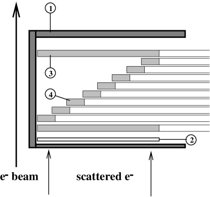
Figure 1: Schematic set-up of the tagging box: 1) X-ray shielding, 2) Si microstrip detector, 3)-4) Scintillators and light guides for timing.

Photon energy was provided by an internal tagging system located right after the exit dipole of a straight section (Figure 1). Electron position was measured by a silicon microstrip detector (128 strips with a pitch of 300 $\mu$m and 500 $\mu$m thick). Two long plastic scintillators covering the whole focal plane (38.4 mm) and 8 small ones, each covering $\approx$1/8 th, were situated behind the microstrip detector and provided a fast signal capable of separating 2 electrons of adjacent bunches (2.8 ns difference) and used as START signal in all Time of Flight (ToF) measurements of the experiment. The whole system was embedded in a 4$\pi$ shielding box (equivalent to 8 mm Pb) against the huge X-ray back-ground. The thickness of this box and the minimum distance allowed to the electron beam determined our threshold of 650 MeV in gamma-ray energy.

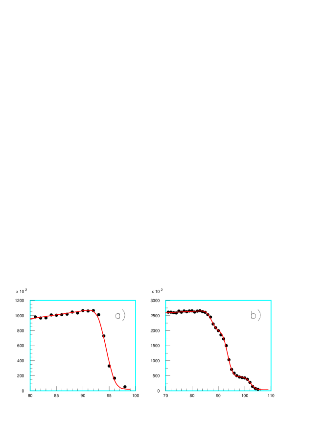
Figure 2: Analysis of the Compton edge for visible laser light (a) and u.v.light (b).

The CE measured by the silicon microstrip detector is displayed on Fig.2 both for the visible and u.v. light provided by the laser. The CE is fitted for a given laser wave length by the function

$$N(X)=a_{1}(1+a_{5}X)\left(1-{\rm erf}(X)\right)+a_{4}$$ (7)

for $X<0$, and

$$N(X)=a_{1}\left(1-{\rm erf}(X)\right)+a_{4}$$ (8)

for $X>0$, where $X=\frac{x-a_{2}}{a_{3}\sqrt{2}}$ and where $x$ is the position (expressed in microstrip number). The parameters $a_{1}$ to $a_{5}$ are fitted to the experimental spectrum, $a_{2}$ represents the CE position and $a_{3}$ the Gaussian parameter $\sigma$, $a_{1}$ is the amplitude, $a_{3}$ is the slope of the spectrum below the (CE) and $a_{4}$ is the residual gamma spectrum after the CE. The residual gamma spectrum is due to the Bremstrahlung of the electron beam. For u.v. three different groups of laser lines: 334.4, 351.1 and 335.8 nm, are present and can be seen on the experimental spectrum.

As shown in Figure 2, the experimental energy resolution can be extracted from the fit of the Compton edge, the theoretical distribution ending abruptly. In the case of u.v. lines (Figure 2b) the three edges are clearly resolved and their peak position, width and relative intensity can be obtained. The measured resolution (FWHM$\simeq$16 MeV) is in agreement with the estimated one from the simulation and is dominated by the electron beam energy dispersion (FWHM=14 MeV). The peak position is used to calibrate and monitor the absolute position of the microstrip detector whereas the relative laser line intensities are input to the calculation of the $\gamma$-ray beam polarization.

Typically an accuracy of $\simeq 0.03$ microstrip is obtained for the position of a given line (parameter $a_{2}$ ). This value corresponds to $\simeq 0.2MeV$ and thus

$$\Delta{E_{\gamma}}/E_{\gamma}\simeq 2\times 10^{-4}.$$ (9)

As a result 2075 measurements have been performed from 10.04.1998 to 11.05.2002 split in 48 periods of measurements.

4 Data Analysis

A special interactive software has been developed for the analysis of the GRAAL data. The data in our disposal have been represented via sequence of blocks with equal values of the Compton edge, as shown in Table 1.

Block	CE	Laser	Date of	Total	Months(1998-2002)/Number of measurements
	position	nm	measurements	points	I	II	III	IV	V	VI	VII	VIII	IX	X	XI	XII
1	54.7-56.5	514.5	05.06.1999-	389	26	39	-	-	-	151	-	-	94	79	-	-
			05.02.2002
2	94.2-94.8	351.1	10.04.1998-	443	-	-	-	87	62	64	32	60	138	-	-	-
			21.09.1998
3	101.3-101.9	351.1	16.04.1999-	316	-	-	-	192	124	-	-	-	-	-	-	-
			16.05.1999
4	104.4-104.9	351.1	30.01.2000-	209	6	145	58	-	-	-	-	-	-	-	-	-
			06.03.2000
5	108.0-110.7	334.4,	15.04.2000-	329	-	39	69	97	8	-	-	-	-	-	116	-
		351.1	12.03.2002
Total	53.1-110.7		10.04.1998-	2075	32	261	180	546	256	215	32	60	298	79	116	-
			11.05.2002

Table 1: The dates of the different measurements which contribute to the final analysis.

For each block the extreme values, the dates of the start and the end of measurement are given in Table 1. The table shows also the distribution of the periods of measurements over months. All existing data have been studied by means of the normalization by dividing the Compton edge values of each of 48 initial data fragments. Variations both within 24 hour day and sidereal day have been studied.

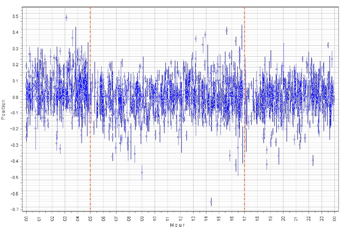
Figure 3: Experimental data plotted as a function of hour, showing their daily variation. The dispersion of data around the average, taken arbitrarily at zero, is expressed in fractions of microstrip (300 micrometers width or about 7 MeV for one microstrip).

Though large dispersion is apparent, see Figure 3, most of the experimental points are located within $\pm 0.3$ microstrip and a stability with accuracy $2\times 10^{-3}$ can be estimated from the rough data.

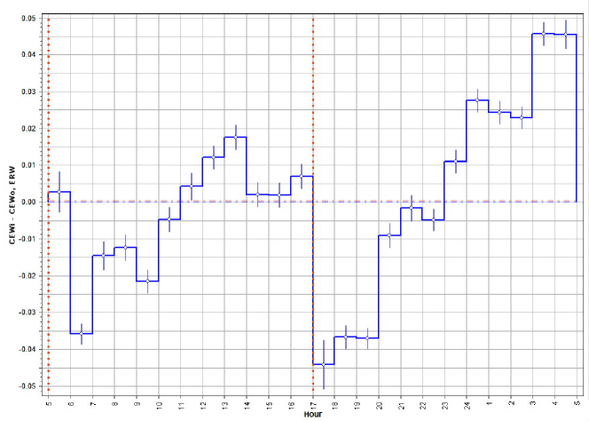
Figure 4: The same as Figure 3, but each point is the average over one hour. The dotted lines show the refill time of the machine corresponding to a possible change in temperature of the tagging detector. The average is also expressed in microstrip fractions.

Figure 4 shows the daily variations of data averaged over 1 hour intervals. The quasi-monotonous increase of the average energy after the filling every 12 hour (vertical bars) is clearly distinguished. This effect could be understood as a change in temperature of the beam vessel and therefore a change in position of the tagging box with respect to the beam. The correlation is obvious, but at a low level: 0.09 microstrip over 12 hours i.e. three times the uncertainty on a single measurement. However, this effect is averaged out at our main goal, i.e. when we look at the data as a function of CMB dipole position.

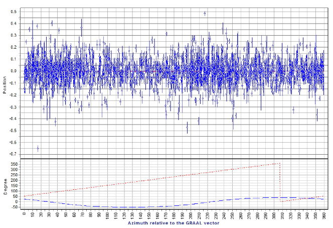
Figure 5: Experimental data plotted as a function of the azimuth (above); below, the variation of the angle between the beam and the CMB dipole decomposed to azimuth (dotted) and declination (dashed) angles is shown. Dispersion has the same expression as for the two previous figures.

The variation of the data over the azimuth angle is shown in Figure 5, together with the variation of the angular distance between the beam and the apex of the CMB dipole. Note the existence of up to 10 $\sigma$ fluctuations for the individual points which we could not correlate to any systematic effect.

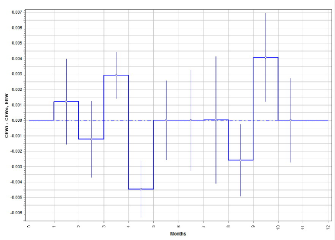
Figure 6: Experimental data over 12 month period averaged by month. The average, also expressed in microstrip fractions, is found very close to zero.

The distribution of all data averaged by month is given in Figure 6. As can be seen in that plot, the averaging procedure gives very low values for the fluctuations, showing that the daily fluctuations observed in Figure 4 are averaged out. From this plot we can estimate the fluctuations to $\simeq 0.015\pm 0.007$ microstrip corresponding to

$$\Delta E_{\gamma}/E_{\gamma}\simeq(1\pm 0.5)\times 10^{-4}.$$ (10)

The uncertainty is statistical only and reflects the averaging procedure.

5 Conclusions

From the stability limit shown in Figure 6, we established the following constraint for the light speed anisotropy: $\Delta c/c\leq(1\pm 0.5)\times 10^{-12}.$ The systematic errors of the experiment are indeed very difficult to estimate, thus in view of the large and unexplained fluctuations of the fitted value for the CE, we adopt a conservative limit

$$\Delta c/c<3\times 10^{-12}.$$ (11)

However, even this conservative limit is about 3 orders of magnitude better than the one reachable from measurements involving the space probes (including the Cassini probe), since it will correspond to several meter accuracy for a planetary orbit; also it deals with one-way effect, while the space measurements are two-way ones (Nordtvedt, personal communication, 2004).

It is important to note that, the electrons are circulating inside the machine at a rate of $10^{6}$ revolutions per second, and therefore, an anisotropy effect cannot be compensated by the stabilization procedure of the machine as it could happen in a linear accelerator. In other words, the angle between the electron speed inside the ring and the direction of the CMB dipole is changing so fast, that the machine cannot compensate for a change in energy induced by an anisotropy.

Further studies of the light speed anisotropy with respect to the apex of CMB dipole, possibly in dedicated experiments with higher $\gamma$ and lower $d\gamma$, seem crucial and can reduce our limit or give evidence for possible anisotropy effects.

We thank K.Nordtvedt for valuable discussions and the ESRF teams for their permanent help, in particular, L.Hardy, J.L.Revol, D.Martin and the members of the alignment group.

References

- [1] Gurzadyan V.G., Margarian A.T., Physica Scripta, 53, 513, 1996.
- [2] Bennett C.L., et al., ApJ Suppl. 148, 1, 2003.
- [3] Rauzy S., Gurzadyan V.G., Mon. Not. Roy. Astr. Soc., 298, 114, 1998.
- [4] Harutyunian F.R., Tumanian V.A. Phys.Lett. 4, 176, 1963; Milburn R.H., Phys.Rev.Lett. 10, 75, 1963.
- [5] Bocquet J.P. et al. Nucl. Phys. A622, 125, 1997.
- [6] Nedorezov V.G., Turinge A.A., Shatunov Yu.M. Physics-Uspekhi, 47, 341, 2004.
- [7] Will C.M. Phys.Rev.D., 45, 403, 1992.
- [8] Riis E. et.al. Phys.Rev.Lett. 60, 81, 1988; Bay Z. and White J., ibid. 62, 841, 1989.
- [9] Vessot et al.,Phys.Rev.Lett. 45, 2081, 1980.
- [10] Krisher T.P et al.,Phys.Rev.D 42, 731, 1990.
- [11] Schaefer B.E. Phys. Rev. Lett. 82, 4964, 1999.
- [12] MacArthur D.W. Phys.Rev.A 33, 1, 1986.